Atom Optics Quantum Pendulum

Abstract

We explain the dynamics of cold atoms, initially trapped and cooled in a magneto-optic trap, in a monochromatic stationary standing electromagnetic wave field. In the large detuning limit the system is modeled as a nonlinear quantum pendulum. We show that wave packet evolution of the quantum particle probes parametric regimes in the quantum pendulum which support classical period, quantum mechanical revival and super revival phenomena. Interestingly, complete reconstruction in particular parametric regime at quantum revival times is independent of potential height.

I Introduction

Pendulum in quantum mechanics Condon is a subject of great interest when the question comes to explain hindered internal rotations in chemistry Lister , quantum features of scattering atoms in quantum optics Dyrting ; Chu , perturbation theory methods to study weak field effects in quantum mechanics Schwartz ; Jhonston ; Kiang , dynamics of Bose-Einstien condensates in optical lattices for small nonlinearityH.Pu and many other physical systems. Comprehensive study of quantum pendulum has brought to light its various aspects which include the structure of energy spectrum, the time evolution focusing on the quantum revivals WRevivals ; Robinett ; Doncheski ; Saif and asymptotic Mathieu solutions using algebraic methods Frenkel .

Super cold atoms in optical standing field is an area of both theoretical and experimental interest and modeled as quantum pendulum Dyrting . The system is of great importance in classical and quantum domain as an explicit time dependence in phase or amplitude makes the classical counterpart chaotic.

Bose-Einstein condensates in an optical lattice Morsch is a mile stone and an important paradigm to study atomic condensate evolution, and its phase transition from Mott insulator to superfluid state MAP Fisher ; Wright ; Jaksch ; Greiner ; BlochJPB ; Eckardt ; Bloch . Quantum revivals in the system present a profound manifestation of quantum interference. The phenomenon occurs as optical lattice potential is not perfectly harmonic and level spacing varies with quantum number. The revivals provide useful information about the coherence time of the atoms in the optical lattice.

In Robinett ; Doncheski energy spectrum and time scales encoded in the spectrum are discussed in detail. In this contribution, we extend the work following the same approach and explain the evolution of super cold weakly condensed atoms in time independent optical lattice. Furthermore, we explain the energy spectrum and eigen states of the system both analytically and numerically. The time dynamics of the wave packet also translates the relevance of energy spectrum with classical phase space. We probe distribution of energy eigen states of the potential via wavepacket evolution. For the simplicity we limit our discussion to deep optical lattice where tunneling does not play significant role. We show: (i) An equally spaced local energy spectrum deep in the well which reflects itself in the reconstruction of the wavepacket at classical periods; (ii) Beyond this region, the behavior changes as the level spacing modifies itself. The nonlinear behavior dominates and controls the dynamics as we go farther from the deep-in-the-well condition; (iii) Numerical calculations with enhanced efficiency and accuracy in the presence of analytical relationships explain the detailed dynamics of the quantum pendulum and its parametric dependence on anharmonicity.

In section II, we discuss atomic interaction with optical lattice and obtain quantum pendulum. In section III, we work out analytical solutions of the potential. In section IV, simplified quantum pendulum is modeled as series expansion of cosine potential and effect of each term of the series is explained which plays the effective role in the atomic evolution  in quantum pendulum. Results are discussed in section V.

II The Model

We consider super cold two-level atoms interacting with a classical monochromatic standing wave field, $E(x,t)=\hat{e}_{y}[\varepsilon_{o}\cos(k_{L}x)e^{-i\omega t}+c.c.].$ Here, $\omega$ and $k_{L}$ are, respectively, the frequency and the wave number of the laser field, and $\hat{e}_{y}$ is the polarization vector. We assume that the cavity end mirrors, in $yz$-plane, reflect the incoming light wave along $x$-axis and, therefore, determine the position of the nodes of the standing light along the axis. In dipole and rotating-wave approximations the atom-field interaction is controlled by the Hamiltonian,

$$H=\frac{p_{x}^{2}}{2M}+\hbar\omega_{o}|e\rangle\langle e|-\{\overset{\rightharpoonup}{d}.\hat{e}_{y}\varepsilon_{o}\cos(k_{L}x)\times e^{i\omega t}\sigma_{+}+H.c\}.$$ (1)

Here, $\hbar\omega_{o}$ is the energy difference between atomic excited state, $|e\rangle,$ and ground state, $|g\rangle,$ and $\overset{\rightharpoonup}{d}$ indicates atomic dipole moment. Moreover, $p_{x}$ is the center-of-mass momentum of the atom along the cavity axis, $M$ is the atomic mass and $\sigma_{\pm}$ are the raising and lowering operators defined as; $\sigma_{+}=|e\rangle\langle g|$ and $\sigma_{-}=|g\rangle\langle e|$. Furthermore, we have considered condensate densities so low that interparticle interactions are negligible and single particle approach remain applicable Gardiner ; Eckardt2009 . Thus, we represent the wave function of the system at any time of interaction, $t,$ as, $|\psi\left(x,t\right)\rangle=\psi_{g}\left(x,t\right)|g\rangle+\psi_{e}\left(x,t\right)e^{-i\omega t}|e\rangle$. In the presence of sufficiently large detuning between the atomic transition frequency and the field frequency, i.e., $\delta_{L}=\omega_{0}-\omega,$ allows us to neglect spontaneous emission. Furthermore, the same consideration allows us to eliminate the excited state adiabatically and leads to effectively describe the evolution of the atom within the electromagnetic field in its ground state. Hence the dynamics of an atom, is governed effectively by the Hamiltonian,

$$H=\frac{p_{x}^{2}}{2M}-\frac{\hbar\Omega_{eff}}{8}\cos(2k_{L}x).$$

Here, $\Omega_{eff}=\Omega^{2}/\delta_{L}$ is the effective Rabi frequency, where, $\Omega=\overset{\rightharpoonup}{d}.\hat{e}_{y}\varepsilon_{o}/\hbar$ is Rabi frequency. The probability to find an atom, therefore, in the excited state is negligible as a consequence of large detuning, the evolution properties of the atom in the field are completely determined by the ground state amplitude. It is useful to define the following dimensionless quantities $t=\omega t,$ $\bar{x}=2k_{L}x,$ $p=(2k_{L}/M\omega)p_{x}$ and $\bar{H}=H(4k_{L}^{2}/M\omega^{2}).$ We get the dimensionless effective Hamiltonian as

$$\bar{H}=\frac{p^{2}}{2}-V_{0}\cos\bar{x},$$ (2)

where, the parameters $V_{0}=\epsilon\Omega_{eff}/\omega^{2}$ is the effective potential depth and $\epsilon=\hbar k_{L}^{2}/2M$ is the recoil shift. In case $\delta_{L}\,>0$ and the laser is tuned red to the atomic transition, we find $V_{0}$ as positive. Hence, a phase difference between the potential and laser intensity shifts the location of the potential minima such that they coincide with the locations of the laser intensity maxima. The atom is, therefore, attracted towards the intensity maxima. In the other case, that is $\delta_{L}<0,$ the phase difference between the potential and laser intensity disappears and the atom is attracted towards intensity minima. The quantized system has another controlling parameter as scaled Planck’s constant $k^{-}=8\epsilon/\omega,$ which follows the commutation relation $i[p,\bar{x}]=k^{-}.$ Here, $\bar{H}$ effectively defines the dynamics of a quantum particle as a quantum pendulum.

The eigen states for quantum rotor have the spatial periodicity condition $\phi_{n}(\bar{x})=\phi_{n}(\bar{x}+2\pi),$ while, eigen states for an atom in optical lattice obeys the general Bloch condition $\phi_{n}(\bar{x})=e^{i2\pi\nu}\phi_{n}(\bar{x})$ where $\nu$ indicates the quasi-momentum of the eigen state. The general Bloch condition satisfy the spatial boundary condition for quantum rotor, when $\nu$ has integer values. In contrast, the range of $\nu$ is continuous for optical lattices. In both cases the potential only couples the eigen states on a momentum ladder where the ladder spacing is $2\hbar k_{L}.$ However, for optical lattices, there are many momentum ladders independent from each other while for quantum rotor there is only one, centered at $p=0$ Madison .

III Schrödinger Equation for Quantum Pendulum and Mathieu Equation

The dynamics of the atom interacting with a standing wave field in the large detuning limit is effectively controlled by the time independent Schrödinger wave equation, expressed as

$$-\frac{k^{-2}}{2}\frac{\partial^{2}\psi(\bar{x})}{\partial x^{2}}-V_{0}\cos(x)\psi(\bar{x})=E_{n}\psi(\bar{x}),$$

where, for simplicity we write $\psi_{g}=\psi$ and $\bar{x}\rightarrow x$. We rewrite the position variable $x$ as $x\equiv x-\pi$, and get Mathieu equation,

$$\frac{\partial^{2}\psi_{n}(x)}{\partial x^{2}}+[a_{n}-2q\cos(x)]\psi_{n}(x)=0,$$

which states that for any given $a_{n}$ and $q,$ we have a series of solution, $\psi_{n}(x),$ for the differential equation, labeled by index $n.$ Hence, $\psi_{n}(x)$ defines the eigen function of the system and

$$q\equiv\frac{V_{0}}{k^{-2}}=\frac{\hbar\Omega_{eff}}{64E_{R}}\ \text{and\ }a_{n}\equiv\frac{2E_{n}}{k^{-2}},$$ (3)

express, respectively, effective potential depth and Mathieu characteristic parameter leading to eigen energies.

Atom in an optical lattice may observe deep or shallow potential depths corresponding to its energy. Following equation 3, we scale effective potential depth by recoil energy of an atom, $E_{R}=\hbar\epsilon$. The atom in cosine potential observes a deep optical potential if effective potential depth $V_{0}$ is of the order of a few hundred single photon recoil energies and temperature of the atom is around recoil temperature. In this case the dynamics of the quantum particle in the individual well is independent and one obtains multiple realization of anharmonic oscillators. On the other hand when the depth of the potential is just few recoil energies and atom is at about recoil temperatures,  it sees a shallow potential. In this case, the quantum mechanical effects caused by spatial periodicity of optical lattices such as formation of Bloch waves become important. Furthermore the levels are broadened into bands due to resonant tunneling between adjacent wells Holthaus . Tunneling in the low-lying bands is suppressed as the well depth is increased and particle motion is dominated by single-well dynamics as it is discussed for large $V_{0}$.

A moderate values of $V_{0}$, with an effective Planck’s constant of order unity, indicates the deep quantum regime. The semiclassical dynamics of the atom in the standing wave field are observed however for large values of $V_{0}$, which correspond to small values of effective Planck’s constant $k^{-}$ and here we find several tightly bound energy bands. Quantum mechanical effects for small $V_{0}$, become important once the atomic de Broglie wavelength $\frac{2\pi\hbar}{P}$ significantly exceeds the lattice constant $d=\frac{1}{2}\frac{2\pi}{k_{L}}=\frac{\lambda_{L}}{2}.$ This gives the condition

$$\frac{P^{2}}{2M}\ll\frac{4\hbar^{2}k_{L}^{2}}{2M}\equiv 4E_{R}.$$

For a fixed value of $q$, there are countably infinite number of solutions, labeled by $n.$ However, only for specific characteristic values of the parameter $a_{n}$, the solutions will be periodic, with periods $\pi$ or $2\pi$ in the variable $x,$ which are denoted by $a_{n},$ and $b_{n},$ respectively for the even and odd solutions. Because of the intrinsic parity of the potential, the solutions can be characterized as being even, $ce_{n}(x,q)$ or cosine-like for integral values of $n$, with $n\geq 0.$ Whereas they are odd, $se_{n}(x,q)$ or sine-like for integral values of $n$, with $n\geq 1$. Limiting cases i.e.. $q=0,$ $q\ll 1$ and $q\gg 1$ for quantum pendulum are discussed in detail in Reference Doncheski .

Approximate expressions for the characteristic values of $a_{n}$ and $b_{n}$ both in $q\ll 1$ and in $q\gg 1$ limits are provided by references AbramowitzStegun ; McLachlan . For the limit, $q\ll 1$, we find that the $a_{n}$, $b_{n}$ are approximately degenerate for $n\gtrsim 7,$ that is,

$$a_{n}\simeq b_{n}=n^{2}+\tfrac{q^{2}}{2(n^{2}-1)}+\tfrac{(5n^{2}+7)q^{4}}{32(n^{2}-1)^{3}(n^{2}-4)}+...\text{.}$$ (4)

The above expression is not limited to integral value of $n$ and is a very good approximation when $n$ is of the form, $m+\frac{1}{2}$. In case of integral value of $n=m,$ the series holds only up to the terms not involving $n^{2}-m^{2}$ in the denominator. The difference between the characteristic values for even and odd solutions satisfy

$$a_{n}-b_{n}=O(\tfrac{b_{n}}{n^{n-1}})\text{ \ \ \ \ as }n\rightarrow\infty$$

In other limiting case, when $q\gg 1$ and the spectrum is oscillator like, we find

$$a_{n}\approx b_{n+1}\approx-2q+2s\sqrt{q}-\tfrac{s^{2}+1}{2^{3}}-\tfrac{s^{3}+3s}{2^{7}\sqrt{q}}-..........,$$ (5)

where, $s=2n+1.$ It has, thus, $(n+\frac{1}{2})k^{-}\omega_{h}$ dependence in lower order, which resembles harmonic oscillator energy for $\omega_{h}=2\sqrt{V_{0}}$. Here in the deep optical lattice limit, the band width is defined as AbramowitzStegun

$$b_{n+1}-a_{n}\simeq\tfrac{2^{4n+5}\sqrt{\frac{2}{\pi}}q^{\frac{n}{2}+\frac{3}{4}}\exp(-4\sqrt{q})}{n!},$$ (6)

which shows that in the deep optical lattice ($q\gg 1$ limit) energy bands are realized as degenerate energy levels as the band width is negligible. The band structure of optical lattice is shown in figure-1, for large $q,$ near the bottom of the lattice,thin band are seen, band width increases and band gap decreases as we move towards the top of the lattice potential well.

As a consequence, we suppress atomic tunneling in deep optical lattice limit. The hoping matrix element, $J,$ explain the tunneling between adjacent sites for deep optical lattice Jaksch ; BlochJPB ; Bloch , viz,

$$J=\frac{4}{\sqrt{\pi}}E_{R}(V_{o}/E_{R})^{\frac{3}{4}}\exp(-2\sqrt{V_{o}/E_{R}}).$$ (7)

Equations 6, 7 show that the width of the bands corresponds to tunneling of the atom from one lattice site to the other. In the limit of deep lattice potentials, this probability will be exponentially small and band width therefore, reduces exponentially as a function of lattice potential depth.

Using algebraic methods, asymptotic even mathieu functions are Frenkel given as

$$ce_{n}(x,q)=\tfrac{(n^{4}-6n^{3}+11n^{2}-6n)D_{n-4}+(4n-4n^{2})D_{n-2}-4D_{n+2}-D_{n+4}}{64\sqrt{q}}$$

$$+\frac{1}{1024q}[\frac{1}{8}(n^{8}-28n^{7}+322n^{6}-1960n^{5}+6769n^{4}-13132n^{3}+13068n^{2}-5040n)D_{n-8}-(n^{6}-15n^{5}+85n^{4}$$

$$-225n^{3}+274n^{2}-120n)D_{n-6}+4(n^{5}-7n^{4}+17n^{3}-17n^{2}+6n)D_{n-4}-(n^{4}+26n^{3}-37n^{2}+10n)D_{n-2}+$$

$$(-36-25n+n^{2})D_{n+2}-4(n+2)D_{n+4}+D_{n+6}+\frac{1}{8}D_{n+8}]+D_{n}+O(\frac{1}{q^{\frac{3}{2}}}),$$ (8)

where, in terms of Hermit polynomials $D_{n}(\alpha)=\frac{1}{2^{\frac{n}{2}}}\exp(-\frac{\alpha^{2}}{4})H_{n}(\frac{\alpha}{\sqrt{2}})$and $\alpha$ is defined as $\alpha=2q^{\frac{1}{4}}\cos(x).$ The normalization factor for $ce_{n}(x,q)$ up to order $O(\frac{1}{q^{2}})$ is

$$\tfrac{1}{C_{n}^{2}}=\tfrac{\sqrt{2}n!}{\sqrt{\pi}q^{\tfrac{1}{4}}}[1+\tfrac{2n+1}{8(\sqrt{q})}+\tfrac{n^{4}+2n^{3}+263n^{2}+262n+108}{2048q}+\tfrac{6n^{5}+15n^{4}+1280n^{3}+1905n^{2}+1778n+572}{16384q^{\frac{3}{2}}}+o(\tfrac{1}{q^{2}})],$$ (9)

here eigen states are normalized to $\pi.$

IV Bound States of an Optical Lattice

Around the minima of lattice sites harmonic evolution prevails and in the presence of the higher order terms it gradually modified to the original potential. Microscopic investigation of the atom-optical system, using term by term contribution of cosine potential expansion reveals the dominant role of the system’s particular parametric regime in the formation of eigen-states and eigen energies. This leads to simplified analytical solutions around the potential minima in the system, as discussed below.

IV.1 Harmonic Oscillator Like Limit.

In the deep lattice limit, the potential near the minima can be approximated as quadratic. Thus the particle placed near the minima of the cosine potential, experiences a harmonic potential. The energy in this regime is obtained as, $E_{n}^{(0)}=(2n+1)k^{-}\sqrt{V_{0}}-V_{0},$ which can be identified in equation 5, by ignoring square and higher powers in $s.$ The eigen states of quadratic potential are given as $\phi_{n}(x)=\sqrt{\frac{\beta}{2^{n}n!\sqrt{\pi}}}H_{n}(\beta x)\exp(\frac{-\beta^{2}x^{2}}{2}),$ where, $H_{n}(\beta x)$ are Hermite polynomials and $\beta=(\frac{2\sqrt{V_{0}}}{k^{-}})^{\frac{1}{2}}=\sqrt{2}q^{\frac{1}{4}}.$

The time evolution of the particle, initially in state $\psi(x,0),$ is obtained by time evolution operator $\hat{U},$ such that, $\psi(x,t)=\hat{U}\psi(x,0)=\sum\limits_{n=0}^{\infty}c_{n}\phi_{n}(x)\exp(-i\frac{E_{n}}{k^{-}}t),$ where, $E_{n}$ and $\phi_{n}(x)$ are energy eigen values and eigen states corresponding to quantum number, $n.$ The probability amplitudes $c_{n}$ are defined as, $\langle\phi_{n}(x)|\psi(x,0)\rangle.$ The quantum particle wave packet in optical potential, narrowly peaked around a mean quantum number $\bar{n},$ displays quantum recurrences at different time scales, defined as$\ T_{(j)}=\frac{2\pi}{(j!k^{-})^{-1}E_{n}^{j}|_{n=\bar{n}}},$ where, $E_{n}^{j}$ denotes the $j^{th}$ derivative of $E_{n}$ with respect to $n$. The time scale, $T_{(1)},$ is termed as classical period as it provides a time at which the particle completes its evolution following the classical trajectory and reshapes itself. Whereas, at$\ T_{(2)}$ the particle reshapes itself as a consequence of quantum interference in a nonlinear energy spectrum, which is purely a quantum phenomenon and thus named as quantum revival time. In the parametric regime of a changing nonlinearity with respect to quantum number, $n,$ we find, the super revival time $T_{(3)}$ for the quantum particle LeichtleAverbukhSchleich .

We study the time evolution of the material wave packet using square of the autocorrelation function Nauenberg ,

$$|A(t)|^{2}=\sum\limits_{n=0}^{\infty}|c_{n}|^{4}+2\sum\limits_{n\neq m}^{\infty}|c_{n}|^{2}|c_{m}|^{2}\cos[(E_{n}-E_{m})\frac{t}{k^{-}}].$$

In the present parametric regime the square of the autocorrelation function is written as

$$|A(t)|^{2}=\sum\limits_{n=0}^{\infty}|c_{n}|^{4}+2\sum\limits_{n\neq m}^{\infty}|c_{n}|^{2}|c_{m}|^{2}\cos((n-m)2\sqrt{V_{0}}t),$$ (10)

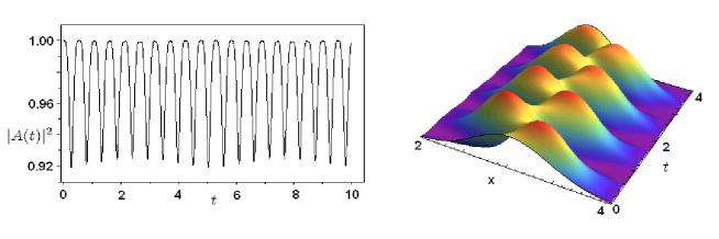
Figure 2: Time evolution of particle wave packet placed at the bottom of the cosine  potential. The dimensions of the wave packet are $k^{-}=0.5,$ $\Delta p=0.5$ with $V_{0}=10.$ We show autocorrelation function vs time (right side) and spatiotemporal behavior of the material wavepacket (left side). The wave packet see equally spaced energy levels and rebuilds after every classical period. Analytically calculated value of classical period and numerical results show an excellent agreement.

where, $\sum\limits_{n=0}^{\infty}|c_{n}|^{4}$ is independent of time, and defines the interference free, averaged value of $|A(t)|^{2}$. The most dominant contribution to the $|A(t)|^{2}$ comes from $n-m=1$ in the second part at the right side of equation 10. Other terms with, $m-n\geq 1,$ have negligible role because their oscillation frequency is an integral multiple of fundamental frequency $2\sqrt{V_{0}},$ and are averaged out to zero. For the reason the square of the autocorrelation function in the present case oscillates following a cosine law with a frequency $2\sqrt{V_{0}}$ which leads to a classical time period $T_{cl}^{(0)}=\frac{\pi}{\sqrt{V_{0}}}$ as shown in figure 2. Here, zero in the superscript of $T_{cl}^{(0)}$ defines the system’s classical period in the absence of perturbation. At the integral multiples of classical period, $|A(t)|^{2}$ is unity, whereas, at time, which is odd integral multiple of the half of the classical period

$$|A(t)|^{2}=\sum\limits_{n=0}^{\infty}|c_{n}|^{4}+2\sum\limits_{n\neq m}^{\infty}|c_{n}|^{2}|c_{m}|^{2}\cos[(n-m)\pi].$$

Here $\cos[(n-m)\pi]\$has alternatively values $+1$ and $-1,$ when $n-m$ is an even or odd respectively. Thus after the cancellation of positive terms with the negative ones, second summation reduces to minimum value and $|A(t)|^{2}$ attains its minima. Here, in the eigen states expansion

$$\psi(x,t)=\exp[-i(2\sqrt{V_{0}}-\frac{V_{0}}{k^{-}})t]\sum\limits_{n=0}^{\infty}c_{n}\phi_{n}(x)\exp(-i2n\sqrt{V_{0}}t),$$ (11)

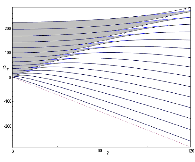
Figure 1: Characteristic values for the Mathieu equation, $a_{2m}$ (for even solutions, blue (grey) curves) and $b_{2m}$ (for odd solutions, red (dark) curves, mostly overridden by blue curves) versus $q$ for the quantum pendulum: The dotted lines correspond to characteristic parameter $a_{n}=\pm 2q$ i.e. $E=\pm V_{0}.$ Note that for a given value of $q$ where $q\gg a_{n},$ the gap between the lowest energy state (lowest solid curve) is roughly one-half of the spacing between solid and dashed curves, corresponding to the zero-point energy in the oscillator limit.

it is notable that the eigen states $\phi_{n}(x)$ have parity $(-1)^{n}.$ In case of even parity, only the even terms $c_{2n}$ are nonvanishing and $n$-dependent exponent factor oscillates two times faster than the general case. At half of classical period the wave packet reappears towards other turning point of the well. In case the wave packet is initially placed at the center of the cosine well, it reappears at half classical period at the same position but in opposite direction. In this case we see classical revivals of the initial atomic wavepacket and quantum revivals take place at infinitely long time. Hence, we find revival of the atomic wavepacket after each classical period only. Experimentally we may realize the situation by placing very few recoil energy atoms deep in the cosine potential well. This reveals the information about the level spacing around the bottom of the cosine potential. Interestingly we find an equal spacing between the energy levels from figure 1, for large $q$ and small value of $n.$ The spatiotemporal behavior of  the wave packet in the quadratic potential, as shown in figure 2, confirms the above results.

IV.2 Quartic Oscillator Limit.

Beyond harmonic oscillator limit, we find oscillator with nonlinearity and energy level spacing different from a constant value. The correction to the energy of harmonic oscillator comes from the first order perturbation (see appendix for energy corrections), that is, $E_{n}^{(4)}=-\frac{k^{-2}}{8}(2n^{2}+2n+1),$ which again can be identified in equation 5 by ignoring cubic and higher order powers in $n.$ The atoms with little higher energy, which is equivalent to several recoil energies observe another time scale in which it reconstructs itself beyond classical period, i.e. quantum revival time. The behavior of auto-correlation function for the wavepacket exactly placed in this region, where only first order correction is sufficient, is shown in figure 3. We see that the wave packet displays revivals at quantum revival time. Thus, little above from the bottom of the of an optical lattice, the wave packet sees variations in energy level spacing in a non-linear fashion. The classical time is modified as $T_{cl}^{(1)}=\alpha^{(1)}T_{cl}^{(0)},$ where $\alpha^{(1)}=1+\frac{\bar{s}}{8\sqrt{q}}$, and classical periodicity for a particle in present situation is related to potential height and mean quantum number, here, $\bar{s}=2\bar{n}+1.$ As $\bar{n}$ increases, classical revival time also increases, and the ratio, $\frac{\bar{s}}{8\sqrt{q}},$ is always less than unity in the region where first correction is sufficient. The quantum revival time, $T_{rev}^{(1)}=\frac{8\pi}{k^{-}},$ is independent of mean quantum number $\bar{n},$ whereas super revival time in this case is infinite.

The eigen states of quartic oscillator due to first order perturbation are given as $\phi_{n}^{q}(x)=\phi_{n}(x)+\phi_{n}^{(1a)}(x),$where, $\phi_{n}^{(1a)}(x)$ is first order correction to the harmonic oscillator wave function and is defined as

$$\phi_{n}^{(1a)}=D_{1}(\eta_{1}\phi_{n-4}+\eta_{2}\phi_{n-2}-\eta_{3}\phi_{n+2}-\eta_{4}\phi_{n+4}).$$ (12)

Here, $D_{1},$ $\eta_{1},$ $\eta_{2},$ $\eta_{3}$ and $\eta_{4}$ are constants and defined in appendix.

In figure 4 eigen states of quadratic, quartic, sixtic and octic oscillators are mapped on numerically obtained eigen states of cosine potential. From this figure we see that for $V_{0}=10$ and $k^{-}=0.5,$ first order correction to the eigen states of unperturbed system matches with harmonic oscillator eigen states up to $n=3,$ and mapping of quartic oscillator with exact solution is much improved compare to harmonic oscillator. Similarly mapping of sixtic oscillator is better than quartic oscillator and is quite good for octic oscillator for all bound band. In this case eight bands exist in side the potential. From figure 1 we note that by increasing $q$ number of bound bands can be increased.

The square of autocorrelation function in this case takes the form

$$|A(t)|^{2} = \sum\limits_{n=0}^{\infty}|c_{n}|^{4}+2\sum\limits_{n\neq m}^{\infty}|c_{n}|^{2}|c_{m}|^{2}\cos[(n-m)2\sqrt{V_{0}}t+(m-n)(n+m+1)\frac{k^{-}}{4}t].$$ (13)

Here, nonlinear dependence of energy eigen values on quantum number, $n,$ makes the argument of cosine function non-linear, as appears in the last term of the above expression. The nonlinear term $(m-n)(n+m+1)$ removes a degeneracy present for the harmonic case between the cosine waves corresponding to nearest neighbouring off diagonal terms and beyond. Hence, there overall evolution display a gradual decoherence leading to collapse which latter transforms in revival as the decoherence in waves disappears. The values of $|A(t)|^{2}$ in this regime at $T_{rev}=\frac{8\pi}{k^{-}}$ is simplifies as

$$|A(t)|^{2}=\sum\limits_{n=0}^{\infty}|c_{n}|^{4}+2\sum\limits_{n\neq m}^{\infty}|c_{n}|^{2}|c_{m}|^{2}\cos[16\pi\sqrt{q}(n-m)].$$ (14)

The equation 14 displays that $|A(t)|^{2}=1,$ when $\sqrt{q}$ is an integral multiple of $\frac{1}{8}$ and also $|A(t)|^{2}$ is unity at half of the revival time if $\sqrt{q}$ is an integral multiple of $\frac{1}{4}$. In case the $\sqrt{q}$ is not an integral multiple of $\frac{1}{8}$, the wave packet revival occurs little earlier than the revival time $T_{rev}=\frac{8\pi}{k^{-}}$ and also $|A(t)|^{2}$ approaches to unity little earlier than $\frac{T_{rev}}{2}$. Here reproduction of wave packet at $\frac{T_{rev}}{2}$ is out of phase by $\pi,$ i.e. at that time all the waves are moving exactly in opposite directions as initially they were. But at $T_{rev}$ they are all moving in same direction and each wave is in phase not only with there initial states but also with each other.

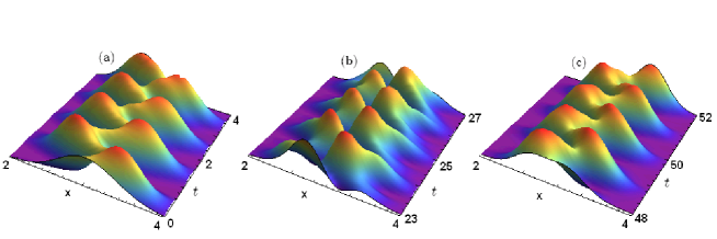
Figure 5: The time evolution of a localized wave packet in a cosine potential is displayed for the same parameters as in figure 2. For short times the initial wavepacket shows classical revivals (a), but starts to display sub-wave-packets in its long time dynamics (b), which constructively interfere at quantum revival time $T_{rev}$ (c). Our analytical and numerical results are in very good agreement.

Figure 5 shows spatiotemporal behavior of the wave packet in cosine potential. We see that wave packet spreads and oscillates in the cosine well, and after some time the original wavepacket is divided into sub-wave-packets figure 5(b). At a quantum revival time these sub-wave-packets constructively interfere and wave packet gains the original shape at the same initial position figure 5(c). At quantum revival time, same classical pattern is seen as at the start of the time evolution shown in figure 5(a).

IV.3 Sixtic Oscillator Limit: Existence of Super Revivals and Beyond

Higher order nonlinearity in the energy spectrum of the quantum pendulum show up beyond quartic limit. In the presence of the second correction, the energy is modified by the term $E_{n}^{(6)}=-\frac{k^{-3}}{\sqrt{V_{0}}}\frac{(2n^{3}+3n^{2}+3n+1)}{32}.$ Second correction to the energy modifies the time scales. The classical time period is now $T_{cl}^{(2)}=\alpha^{(2)}T_{cl}^{(0)},$ whereas the quantum revival time is modified as $T_{rev}^{(2)}=|\beta^{(1)}|T_{rev}^{(1)}.$ Here, $\alpha^{(2)}=\alpha^{(1)}+\frac{3(\bar{s}^{2}+1)}{2^{8}q},$ $\beta^{(1)}=\frac{3\bar{s}}{16q}-1$ are constants. In addition system shows another time scale, i.e. super revival time $T_{spr}^{(2)}=\frac{64\pi\sqrt{V_{0}}}{k^{-2}},$ at which reconstruction of original wave packet takes place. The other quantum revival times occur at infinity.

The energy eigen states in this regime are given as $\phi_{n}^{(s)}=\phi_{n}+\phi_{n}^{(1,a)}+\phi_{n}^{\left(1,b\right)}+\phi_{n}^{\left(2,a\right)},$ where, $\phi_{n}^{\left(2,a\right)}$ is perturbation in eigen states due to the $H^{(6)}$ term and $\phi_{n}^{\left(1,b\right)}$ is second order perturbation caused by $H^{(4)}$ term Doncheski . The expressions $\phi_{n}^{\left(1,b\right)}$ and $\phi_{n}^{\left(2,a\right)}$ are given as

$$\phi_{n}^{\left(1,b\right)} = D_{2}[\delta_{1}\phi_{n-8}+\delta_{2}\phi_{n-6}+\delta_{3}\phi_{n-4}+\delta_{4}\phi_{n-2}+\delta_{5}\phi_{n+2}+\delta_{6}\phi_{n+4}+\delta_{7}\phi_{n+6}+\delta_{8}\phi_{n+8}],$$

and

$$\phi_{n}^{\left(2,a\right)} = D_{6}[\chi_{{}_{1}}\phi_{n-6}+\chi_{{}_{2}}\phi_{n-4}+\chi_{{}_{3}}\phi_{n-2}+\chi_{{}_{4}}\phi_{n+2}+\chi_{{}_{5}}\phi_{n+4}+\chi_{{}_{6}}\phi_{n+6}].$$

The constants $D_{2},D_{6},\delta_{j}$’$s$ and $\chi_{j}$’$s$ are calculated in appendix, where, $j$ takes integral values.

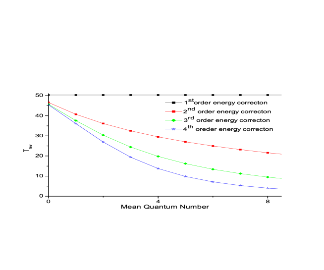
Figure 6: The quantum revival time vs mean quantum number is shown for simplified potentials. In the presence of only first order correction, i.e. for quartic potential, the quantum revival time is a constant. For higher order corrections it decreases with increasing mean quantum number.

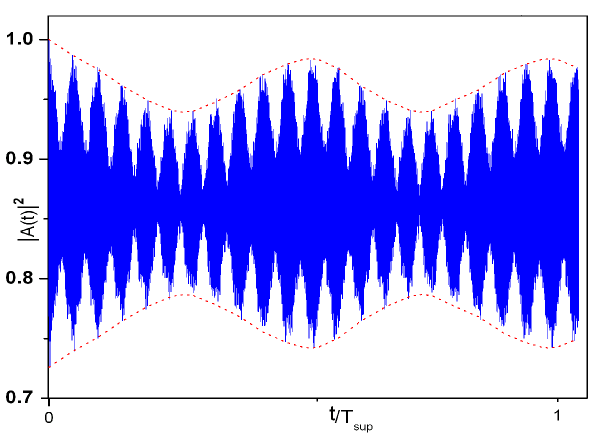
Figure 7: The wave packet dynamics in sixtic potential displays three time scales, the classical periods (making the dense region), the quantum revival times (making the peaks in the dense region) and the super revival times (making the peaks in the envelop of the quantum revivals). The parametric values are the same as in figure 2.

Again in this region classical time increases by increasing $\bar{n}$ and increases faster than as it was in quartic limit. However, in the present regime, the quantum revival time is not constant and decreases as $\bar{n}$ increases. The $\bar{n}$ dependence of quantum revival time is shown in figure 6. The super revival time is independent of mean quantum number. It is directly proportional to square root of potential height and inversely proportional to the square of scaled Planck’s constant. The temporal behavior of an atom in optical potential placed in this regime shows three time scales: classical periods enveloped in quantum revivals and quantum revivals enveloped in super revivals as shown in figure 7. After each super revival time the atomic wave packet evolution repeats itself.

Similarly third correction in energy, modify the energy by the factor $E_{n}^{(8)}=-\frac{k^{-4}}{V_{0}}\frac{(5n^{4}+10n^{3}+16n^{2}+11n+3)}{2^{8}}$. The time scales in this case are $T_{cl}^{(3)}=\alpha^{(3)}T_{cl}^{(0)}$ and$\ T_{rev}^{(3)}=|\beta^{(2)}|T_{rev}^{(1)}$ Where $\alpha^{(3)}=\alpha^{(2)}+\frac{(5\bar{s}^{3}+17\bar{s})}{2^{11}q^{\frac{3}{2}}}\$and $\beta^{(2)}=\beta^{(1)}+\frac{15\bar{s}^{2}+17}{2^{8}q}$ and super revival time is $T_{spr}^{(3)}=|\gamma|T_{spr}^{(2)}$ where $\gamma=\frac{5\bar{s}}{8\sqrt{q}}-1.$ Furthermore, the super quartic revival time, $T_{4}$, is independent of $\bar{n}$. The higher order corrections in energy show that other time scales do exist in the system, but their times of recurrence are too large to consider them finite.

In the presence of third correction to energy, classical time increases as $\bar{n}$ increases but increases little faster than in the cases of quartic and sixtic corrections, whereas, the quantum revival time decreases faster as $\bar{n}$ increases compared to the case of sixtic correction. The super revival time is not constant but decreases as $\bar{n}$ increases.

Energy corrections increase anharmonicity in the system. We discussed that the first order correction to harmonic potential energy led to the quantum revivals, the second order energy correction led to super revivals and fourth correction led to quartic revival time. Comparison of revival times for different energy corrections is shown in figure 6. For first order energy correction quantum revival time is constant, but for higher order corrections, revival time may decrease with increasing mean quantum number of the wavepacket.

In figure 4 we show the projection of numerically calculated eigen states of cosine potential on the eigen states of quadratic, quartic (first correction to quadratic potential), sixtic (second correction to quadratic potential) and octic (third correction to quadratic potential) potentials. We note that the eigen states of all above mentioned potentials match to the eigen states of quadratic potential near the bottom of lattice potential. For little large quantum numbers, we see that projection of quadratic potential falls sharply and improves with higher order potentials. This correction is quite good for octic potential when $q=40$ justifying $q>>1$ condition. Eigen states and eigen energies of quartic, sixtic and octic potentials are analytically calculated using the method given in appendix.

V Discussion

In this paper we have extended the understanding of eigen energy levels and eigen states in deep optical lattice, both analytically and numerically. We note that solutions obtained through perturbation theory and Mathieu solution are showing similar results and are in very good agreement with exact numerical solutions. The energy levels are equally spaced near the bottom and by increasing the lattice potential depth, the number of equally spaced energy levels can be increased. A wave packet placed in this region revives after each classical period. From figure 4, it is also noted that all potentials discussed have equally spaced eigen levels at the bottom of the potential well as their mapping with harmonic oscillator is unity. Beyond linear regime, energy dependence is quadratic and any wavepacket evolved in this region shows complete quantum revivals enveloped by classical revivals. Interestingly in this regime quantum revival time ($T_{rev}^{(1)}=\frac{8\pi}{k^{-}}$) is independent of potential height, however has inverse proportionality with effective Planck’s constant, $k^{-}$. We show that for deep optical lattice, there is a region in which revivals are independent of lattice depth and this region expands with the increase in lattice depth, however beyond this region quantum revival time is no longer constant but decreases as $\bar{n}$ increases. The higher order time scale, super revival time $T_{spr}^{(2)}=\frac{64\pi\sqrt{V_{0}}}{k^{-2}}$ exists in this region and is independent of $\bar{n}$. Again this region expands as potential height is increased but super revival time in this region is directly proportional to square root of potential height.

Above this region other time scales also exist where super revival time is $\bar{n}$ dependent and decreases as $\bar{n}$ increases but these time scales are too long to consider them finite.

VI Acknowledgement

M. A. and K. N. thank Higher Education Commission Pakistan for financial support through grant No.17-1-1(Q.A.U)HEC/Sch/2004/5681. FS is supported by Higher Education Commission Pakistan through research grant 20-23 R & D/03143, The Abdus Slam International Center for Theoretical Physics, ICTP, Trieste, Italy and Pakistan Science Foundation. He thanks S. Stanislav and G. Ghirardi for fruitful discussions. We thank S. Iqbal, Rameez-ul-Islam, I. Rehman and T. Abbas for useful suggestions.

VII Appendix: Solution of an Arbitrary Potential

An arbitrary potential $U(r),$ around its minima can be solved by taking its Taylor’s expansion Liboff , that is

$$U(r) = U(r_{m})+G^{(1)}(r-r_{m})+G^{(2)}(r-r_{m})^{2}+G^{(3)}(r-r_{m})^{3}+....,$$ (15)

where, $G^{(j)}=(j!)^{-1}\partial^{j}U(r=r_{m})/\partial r^{j}$, and $j$ is an integer. The value of $G^{(j)}$ for odd $j$ is zero as potential is $\cos(x)$ and it is calculated at the potential minima $r=r_{m}$. Thus in the presence of weak nonlinearity the term $G^{(6)}<<G^{(4)}<<G^{(2)}$.

In our analysis we consider the expansion up to second order term as unperturbed Hamiltonian, $H_{0}$. The eigen functions and eigen energies of this Hamiltonian are those of harmonic oscillator. The effect of the higher order terms in Taylor’s expansion is discussed as perturbation to eigen energies and eigen functions of the harmonic oscillator. We express the effective Hamiltonian governing the dynamics of atom around the potential minima as

$$H_{0}\cong\frac{{\hat{p}}^{2}}{2}+U(r_{m})+G^{(2)}(r-r_{m})^{2}.$$ (16)

The eigen functions and eigen energies of the harmonic potential are $\phi_{n}(x)=\sqrt{\frac{\beta}{2^{n}n!\sqrt{\pi}}}H_{n}(\beta x)\exp(\frac{-\beta^{2}x^{2}}{2}),$ and $E_{n}^{(0)}=k^{-}\sqrt{V_{0}}(2n+1)+U(r_{m}),$ where, $H_{n}(\beta x)$ are Hermite polynomials.

The first order correction and second order correction to energy is quite well known. The first order correction to the energy of quadratic potential is $E_{n}^{(p,a)}=\langle\phi_{n}|H^{(p)}|\phi_{n}\rangle,$ and the second order correction is obtained from the relation $E_{n}^{(p,b)}=\sum_{m\neq n}\frac{|\langle\phi_{n}|H^{(p)}|\phi_{m}\rangle|^{2}}{E_{n}^{(0)}-E_{m}^{(0)}}.$ The third order correction is determined by

$$E_{n}^{(p,c)} = \sum_{j\neq n}\sum_{l\neq n}\frac{\langle n|\hat{H}^{(p)}|j\rangle\langle j|\hat{H}^{(p)}|l\rangle\langle l|\hat{H}^{(p)}|n\rangle}{(E_{n}^{(0)}-E_{j}^{(0)})(E_{n}^{(0)}-E_{l}^{(0)})}-\langle n|\hat{H}^{(p)}|n\rangle\sum_{j\neq n}\frac{\langle n|\hat{H}^{(p)}|j\rangle\langle j|\hat{H}^{(p)}|n\rangle}{((E_{n}^{(0)})^{2}-(E_{j}^{(0)})^{2})},$$

where,$\ p=3,4,5,6,........\cdot$

The presence of the perturbation term $H^{(4)},$ leads to the Hamiltonian

$$H=H_{0}+H^{(4)}.$$ (17)

Here, the first order correction to eigen functions, due to the $H^{(4)}$ term, is obtained as

$$|\phi_{n}^{(1a)}\rangle=D_{1}(\eta_{1}\phi_{n-4}+\eta_{2}\phi_{n-2}-\eta_{3}\phi_{n+2}-\eta_{4}\phi_{n+4}),$$ (18)

where, $D_{1}=G^{(4)}(\frac{1}{4\sqrt{q}})^{2}\frac{1}{k^{-}\omega_{h}},$

$$\eta_{1} =\sqrt{n(n-1)(n-2)(n-3)}/4,$$

$$\eta_{2} =(2n-1)\sqrt{n(n-1)},\text{ }$$

$$\eta_{3} =(2n+3)\sqrt{(n+1)(n+2)},$$

$$\text{and }\eta_{4} =\sqrt{(n+1)(n+2)(n+3)(n+4)}/4.$$

Now the eigen functions in the presence of first order perturbation, due to the correction $H^{(4)},$ is given as

$$\phi_{n}^{q}(x)=\phi_{n}(x)+\phi_{n}^{(1a)}(x),$$

and second order correction due to $H^{\left(4\right)}$ term is

$$\phi_{n}^{\left(1,b\right)} =D_{2}[\delta_{1}\phi_{n-8}+\delta_{2}\phi_{n-6}+\delta_{3}\phi_{n-4}+\delta_{4}\phi_{n-2}+\delta_{5}\phi_{n+2}+\delta_{6}\phi_{n+4}+\delta_{7}\phi_{n+6}+\delta_{8}\phi_{n+8}.$$ (19)

Here, $D_{2}=(G^{\left(4\right)})^{2}(\frac{1}{4\sqrt{q}})^{4}(\frac{1}{k^{-}\omega_{h}})^{2},$

$$\delta_{1} = \frac{\sqrt{n\left(n-1\right)\left(n-2\right)\left(n-3\right)\left(n-4\right)\left(n-5\right)\left(n-6\right)\left(n-7\right)}}{32},$$

$$\delta_{2} = \frac{\left(6n-11\right)}{12}\sqrt{n\left(n-1\right)\left(n-2\right)\left(n-3\right)\left(n-4\right)\left(n-5\right)},$$

$$\delta_{3} = \left(2n^{2}-9n+7\right)\sqrt{n\left(n-1\right)\left(n-2\right)\left(n-3\right)},$$

$$\delta_{4} = \frac{\left(56n^{3}-228n^{2}+214n-146\right)}{8}\sqrt{n\left(n-1\right)},$$

$$\delta_{5} = \frac{\left(56n^{3}+396n^{2}+838n+645\right)}{8}\sqrt{\left(n+1\right)\left(n+2\right)},$$

$$\delta_{6} = \frac{(31n^{2}+197n+258)}{16}\sqrt{\left(n+1\right)\left(n+2\right)\left(n+3\right)\left(n+4\right)},$$

$$\delta_{7} = \tfrac{\left(11n+27\right)}{24}\sqrt{\left(n+1\right)\left(n+2\right)\left(n+3\right)\left(n+4\right)\left(n+5\right)\left(n+6\right)},$$

$$\text{and }\delta_{8} = \tfrac{\sqrt{\left(n+1\right)\left(n+2\right)\left(n+3\right)\left(n+4\right)\left(n+5\right)\left(n+6\right)\left(n+7\right)\left(n+8\right)}}{32}.$$

Hence, following the same procedure, the first order correction due to $H^{\left(6\right)}$ term changes the Hamiltonian of the system as

$$H=H_{0}+H^{\left(4\right)}+H^{\left(6\right)}.$$ (20)

Hence the corrected eigen function in presence of correction due to $H^{(4)}$ and $H^{\left(6\right)}$ terms appear as

$$\phi_{n}^{(s)}=\phi_{n}+\phi_{n}^{(1,a)}+\phi_{n}^{\left(1,b\right)}+\phi_{n}^{\left(2,a\right)},$$

where,

$$\phi_{n}^{\left(2,a\right)} =D_{6}[\chi_{{}_{1}}\phi_{n-6}+\chi_{{}_{2}}\phi_{n-4}+\chi_{{}_{3}}\phi_{n-2}+\chi_{{}_{4}}\phi_{n+2}+\chi_{{}_{5}}\phi_{n+4}+\chi_{{}_{6}}\phi_{n+6}.$$

Here, $D_{6}=G^{(6)}(\frac{1}{4\sqrt{q}})^{3}\frac{1}{k^{-}\omega_{h}},$

$$\chi_{{}_{1}} = 6\sqrt{n(n-1)(n-2)(n-3)(n-4)(n-5)},$$

$$\chi_{{}_{2}} = \frac{3}{4}(2n-3)\sqrt{n(n-1)(n-2)(n-3)},$$

$$\chi_{{}_{3}} = \frac{15}{2}(n^{2}-n+1)\sqrt{n(n-1)},$$

$$\chi_{{}_{4}} = \frac{15}{2}(n^{2}+3n+3)\sqrt{(n+1)(n+2)},$$

$$\chi_{{}_{5}} = \frac{3}{4}(2n+5)\sqrt{\left(n+1\right)\left(n+2\right)\left(n+3\right)\left(n+4\right)},$$

$$\chi_{{}_{6}} = 2\sqrt{\left(n+1\right)\left(n+2\right)\left(n+3\right)\left(n+4\right)\left(n+5\right)\left(n+6\right)}.$$

Close to the minima of potential, we can find the eigen energies up to a considerable accuracy by using perturbation theory. The leading correction comes from $H^{(4)}$ using first order and second order perturbation theory respectively. The result is as under:

$$E_{n}^{(4)}=(\alpha_{2}n^{2}+\alpha_{1}n+\alpha_{0})k^{-}\omega_{h},$$

where, $\alpha_{0}=3D_{a},$ $\alpha_{1}=6D_{a},$ $\alpha_{2}=6D_{a},$ $C_{b=}(G^{(3)})^{2}(\frac{1}{4\sqrt{q}})^{3}\frac{1}{k^{-}\omega_{h}}$ and $D_{a}=G^{(4)}(\frac{1}{4\sqrt{q}})^{2}.$ At next order, the first order perturbation of $H^{(6)}$and second order perturbation of $H^{(4)}$ contribute. The result can be written as:

$$E_{n}^{(6)}=(\beta_{3}n^{3}+\beta_{2}n^{2}+\beta_{1}n+\beta_{0})k^{-}\omega_{h},$$

where, $\beta_{0}=3I_{a}-21J_{b},\ \beta_{1}=8I_{a}-59J_{b},$ $\beta_{2}=6I_{a}-51J_{b},$ $\beta_{3}=4I_{a}-34J_{b},$ and $I_{a}=5G^{(6)}(\frac{1}{4\sqrt{q}})^{3}\frac{1}{k^{-}\omega_{h}},$ $J_{b}=2(G^{(4)})^{2}(\frac{1}{4\sqrt{q}})^{2}(\frac{1}{k^{-}\omega_{h}})^{2}.$

At the next higher order, we need to evaluate three contributions; $H^{(8)}$ in first order, $H^{(6)}$ and $H^{(4)}$ in second order and $H^{(4)}$in third order. The energy expression is

$$E_{n}^{(8)}=(\gamma_{4}n^{4}+\gamma_{3}n^{3}+\gamma_{2}n^{2}+\gamma_{1}n+\gamma_{0})k^{-}\omega_{h},$$

where, $\gamma_{0}=3X-12Y-111Z,$ $\gamma_{1}=8X-35Y-347Z,$ $\gamma_{2}=10X-46Y-472Z,$ $\gamma_{3}=4X-22Y-250Z,$ $\gamma_{4}=2X-11Y-125Z,$ and $X=35G^{(8)}(\frac{1}{4\sqrt{q}})^{4}\frac{1}{k^{-}\omega_{h}},Y=30G^{(6)}G^{(4)}(\frac{1}{4\sqrt{q}})^{5}(\frac{1}{k^{-}\omega_{h}})^{2},Z=48(G^{(4)})^{3}(\frac{1}{4\sqrt{q}})^{6}(\frac{1}{k^{-}\omega_{h}})^{2}.$

Now the energy of the system is

$${E}_{n} = E_{n}^{(0)}+E_{n}^{(4)}+E_{n}^{(6)}+E_{n}^{(8)},\text{ or }$$

$$E_{n} = (\kappa_{4}n^{4}+\kappa_{3}n^{3}+\kappa_{2}n^{2}+\kappa_{1}n+\kappa_{0})k^{-}\omega_{h}+U(r_{m}),$$ (21)

where, $\kappa_{0}=\alpha_{0}+\beta_{0}+\gamma_{0}+\frac{1}{2},$ $\kappa_{1}=\alpha_{1}+\beta_{1}+\gamma_{1}+1,$ $\kappa_{2}=\alpha_{2}+\beta_{2}+\gamma_{2},$ $\kappa_{3}=\beta_{3}+\gamma_{3},$ and $\kappa_{4}=\gamma_{4}.$

Figure 3: Autocorrelation function for a particle undergoing quantum revival evolution in time. The parameters are same as in figure 2. The wave packet was placed close to the bottom of the potential well in the regime where first order correction is sufficient, it observes quantum revivals after many classical periods.

Figure 4: comparison of cosine potential with the simplified potentials is made by calculating the projection, S, of the eigen states of the cosine potential on the eigen states of the simplified potentials . For first few quantum numbers, the cosine potential very much resembles to the harmonic potential, however, for higher quantum numbers the higher order corrections to the harmonic oscillator are needed to make the resemblance.

References

- (1) E. U. Condon: Phys. Rev. 31 891 (1928); T. Pradhan, A. V. Khare: Am. J. Phys. 41 59 (1973); R. Aldrovandi and P. L. Ferreira: Am. J. Phys. 48 660 (1980); G. P. Cook and C. S. Zaidin: Am. J. Phys. 54 259 (1986).
- (2) D. G. Lister, J. N. MacDonald and N. L. Owen: Internal Rotation and Inversion (Academic Press London, 1978); W. J. Orville-Thomas(Ed.): Internal Rotation in Molecules (Wiley, New York, 1974); G. Ercolani: J. Chem. Ed. 77 1495 (2000); G. L. Baker, J. A. Blackburn and H. J. T. Smith: Am. J. Phys. 70 525 (2002).
- (3) S. Dyrting and J. G. Milburn: Phys. Rev. A 47 R2484 (1993).
- (4) H. Müller, S. Chiow, S. Chu: Phys. Rev. A 77 023609 (2008).
- (5) M. Schwartz and M. Martin: Am. J. Phys. 26 639 (1958).
- (6) G. L. Jhonston and G. Sposito: Am. J. Phys. 44 723 (1976).
- (7) D. Kiang: Am. J. Phys. 46 1188 (1978).
- (8) H. Pu, L. O. Baksmaty, W. Zang, N. P. Bigelow and P. Meystre: Phys. Rev. A 67 043605 (2003).
- (9) J. H. Eberly, N. B. Narozhny and J. J. Sanchez-Mondragon: Phys. Rev. Lett. 44 1323 (1980); N. B. Narozhny J. J. Sanchez-Mondragon, and J. H. Eberly: Phys. Rev. A 23 236 (1981); G. Rempe H. Walther and N. Klein: Phys. Rev. Lett. 58 353 (1987); J. Parker and C. R. Stroud Jr.: Phys. Rev. Lett. 56 716 (1986); J. Yeazell, M. Mallalieu and C. R. Stroud Jr: Phys. Rev. Lett. 64 2007 (1990);T. Baumert, V. Engel, C. Röttgermann, W. T. Strunz and G. Gerber: Chem. Phys. Lett. 191 639 (1992); I. Sh. Averbukh and N. F. Perelman: Phys. Lett. A 139 449 (1989); B. Yurke and D Stoler: Phys. Rev. Lett. 57 13 (1986); B. Yurke and D. Stoler, Phys. Rev. A 35 4846 (1987); A. Mecozzi and P. Tombesi: Phys. Rev. Lett. 58 1055 (1987); D. L. Aronstein and C R Stroud Jr.: Phys. Rev. A 55 4526 (1997); D. L. Aronstein and C. R. Stroud Jr:, Phys. Rev. A. 62 22102 (2000); R. Veilande and I. Bersons: J. Phys. B 40 2111 (2007); I.D. Feranchuk and A.V. Leonov: Phys. Lett. A 373 517 (2009).
- (10) M. A. Doncheski and R. W. Robinnet: Ann. Phys. 308 578 (2003).
- (11) For a review on time evolution of wavepacket in bound systems and quantum revivals, see R W Robinnet: Phys. Rep. 392 1 (2004).
- (12) I. Marzoli, A. Kaplan, F. Saif and W P Schleich: Fortschr. Phys. 56 967 (2008).
- (13) D. Frenkel and R. Portugal: J. Phy. A 34 3541 (2001).
- (14) O. Morsch and M. Oberthaler: Rev. Mod. Phys. 78 189 (2006).
- (15) M. A. P. Fisher, P. B. Weichman, G. Grinstein and D. F. Fisher: Phys. Rev. B 40 546 (1989).
- (16) E. M. Wright, T. Wong, M. J. Collett, S. M. Tan, and D. F. Walls: Phys. Rev. A 56 591 (1997).
- (17) D Jaksch, C. Bruder, J. I. Cirac, C. W. Gardiner and P. Zoller: Phys. Rev. Lett. 81 3108 (1998).
- (18) M. Greiner, O. Mandel, T. Esslinger, T. W. HaÈnsch and I. Bloch: Nature 415 51 (2002).
- (19) I. Bloch: J. Phys. B 38 S269 (2005).
- (20) A. Eckardt, C. Wiss and M. Halthous: Phys. Rev. Lett. 95 260404 (2005).
- (21) I. Bloch, J. Dalibard and W. Zwerger: Rev. Mod. Phys. 80 885 (2008).
- (22) S. A. Gardiner, D. Jaksch, R. Dum, J. I. Cirac and P. Zoller: Phys. Rev. A 62 023612 (2000).
- (23) A Eckardt, M. Holthaus, H. Lignier, A. Zenesini, D. Ciampini, O. Morsch and E. Arimondo: Phys. Rev. A 79 013611 (2009).
- (24) K. W. Madison: Dr. Thesis, The University of Texas at Austin (1996).
- (25) K. Drese and M Holthaus: Chem. Phys. 217 201 (1997).
- (26) M. Abramowitz and I. A. Stegun (eds.) Handbook of Mathematical Functions, Dover, New York 1970 Chap. 20.
- (27) N. W. McLachlan: Theory and applications of Mathieu Functions Oxford university Press London 1947.
- (28) C. Cohen-Tannoudji, J. Dupont-Roc, and Gilbert Grynberg: Atom-Photon Interactions Wiley and Sons, New York 1992.
- (29) C. Leichtle, I. Sh. Averbukh and W. P. Schleich, Phys Rev Lett 77 3999 (1996); C. Leichtle, I. Sh. Averbukh and W P Schleich: Phys. Rev. A 54 5299 (1996).
- (30) M. Nauenberg: J Phys B 23 L385 (1990).
- (31) R. L. Liboff: Introductory Quantum Mechanics (Addison Wesely, New York, 2002) 4th ed.