Glueballs Mass Spectrum in an Inflationary Braneworld Scenario

Abstract

We address the issue of glueball masses in a holographic dual field theory on the boundary of an $AdS$ space deformed by a four-dimensional cosmological constant. These glueballs are related to scalar and tensorial fluctuations of the bulk fields on this space. In the Euclidean $AdS_{4}$ case the allowed masses are discretized and are related to distinct inflaton masses on a 3-brane with several states of inflation. We then obtain the e-folds number in terms of the glueball masses. In the last part we focus on the Lorentzian $dS_{4}$ case to focus on the QCD equation of state in dual field theory.

I Introduction

In the large $N$ limit with the t’Hooft coupling $\lambda=g_{YM}^{2}N>>1$ the $D3$-brane solution of type IIB supergravity leads to an $AdS_{5}\times S^{5}$ spacetime. According to the AdS/CFT correspondence malda97 ; Gubser:1998bc ; witten98 string theory on $AdS_{5}\times S^{5}$ corresponds to a ${\cal N}=4$ superconformal $SU(N)$ gauge theory in $d=4$ dimensions. This holographic correspondence is better understood by working out in the supergravity approximation csaki98 . In the regime of small curvature of the spacetime (i.e. as $g_{YM}^{2}N>>1$) compared to the string and Planck scale, string/M-theory can be well described by supergravity.

The one-to-one correspondence between supegravity on $AdS_{5}\times S^{5}$ and the ${\cal N}=4$ superconformal $SU(N)$ gauge theory fields is given as follows. The mass $m$ of $p$-form field on the AdS space (bulk) has well defined relation with the conformal dimension $\Delta$ of a $(4-p)$ form operator in the dual conformal guge theory on the boundary in the form

$$m^{2}=(\Delta-p)(\Delta+p-4)$$ (1)

In the spectrum of type IIB supergravity on $AdS_{5}\times S^{5}$ there are four singlets of $SO(6)$ which corresponds to glueballs csaki98 . Among them there are the massless graviton $g_{\mu\nu}$ (on the bulk) that couples to the stress-energy tensor $T_{\mu\nu}$ (on the four-dimensional boundary) with conformal dimension $\Delta=4$ and the complex massless scalar field (on the bulk) whose real part is the dilaton that couples to the scalar operators tr$F^{2}$ and tr$F\wedge F$ of the four-dimensional theory (on the boundary) with conformal dimension $\Delta=4$. The other bulk fields are 2 and 4-form fields that we shall not discuss here.

In this paper we shall concentrate in the first two bulk fields. We shall consider a geometry that can be embedded viewed as a $D3$-brane solution in the limit of large $N$. The $D3$-brane geometry and their deformed versions csaki98 are usually used as good dual of glueballs in three dimensional chromodynamics ($QED_{3}$). The gravitational solution we use is the solution of five dimensional braneworld scenario Karch:2001cw ; Karch:2000ct ; Binetruy:1999hy ; Bazeia:2007vx . Here one can understand that we are turning on only the gravitational sector of a type IIB supergravity. The bulk fields here couple to fields with the same conformal dimension on the boundary. This is because in our case the equation of motion for the fluctuations of the metric is formally the same equation for the dilaton field.

These boundary fields are related to glueballs $2^{++}$ and $0^{++}$ and their masses $m^{2}_{2^{++}}=m^{2}_{0^{++}}$ are given by the bulk equations of motion for the gravitational fluctuations and dilaton fields in the gravitational background considered in the braneworld scenario. We point out that the this glueball spectra is also related to the inflaton spectra and we discuss several inflationary states.

II Scenario

In this section we describe a scenario of inflationary braneworld. It will be in this scenario that we will obtain a glueball spectrum by analysing its holographic dual field. This holographic dual field will be identified with an inflaton field.

The inflationary braneworld metric in $d+1$ dimension is given by

$$ds^{2}=\alpha^{\prime}\left[\frac{U^{2}}{R^{2}_{0}}\left(edt^{2}+a_{0}(t)^{2}d\vec{x}_{d-1}^{2}\right)+\frac{R^{2}_{0}}{\left(U^{2}-C\right)}\leavevmode\nobreak\ dU^{2}\right],$$ (2)

where

$$U(r)=({e\gamma+\xi^{2}e^{\mu r}+\chi^{2}e^{-\mu r}})^{\frac{1}{2}},$$ (3)

with $e=-1$, for Lorentzian signature, or $e=+1$, for Euclidean signature, also $\mu=(1/3)(\kappa_{5}^{4}\sigma^{2})^{1/2}$, and

$$\xi^{2}=\frac{1}{2}({1-e\gamma-\sqrt{1-2e\gamma}}\,),\qquad\chi^{2}=\frac{1}{2}(1-e\gamma+\sqrt{1-2e\gamma}\,),$$ (4)

with

$$\gamma=\frac{d-1}{2\sigma}\leavevmode\nobreak\ H^{2},$$ (5)

and also

$$C=2R^{4}_{0}\leavevmode\nobreak\ \gamma,$$ (6)

where $H$ is the Hubble parameter (or the cosmological constant) in the Braneworld, and $T_{brane}=\sigma/\alpha^{\prime d/2}$ is the Braneworld tension. Note that only $\alpha^{\prime}$ is dimensional with $[\alpha^{\prime}]=\textrm{length}^{2}$, and other parameters with $[R_{0}]=[\sigma]=[H]=[x^{\mu}]=1$. The Hubble parameter appears in the braneworld warp factor in terms of the cosmological constant as follows

$$a_{0}(\tau)=\exp(H_{E}\tau),\>\>\>\>H_{E}^{2}\propto-e\Lambda>0,\>e=+1,\>\Lambda<0,\qquad\mbox{(the Euclidean $AdS_{4}$ case)},$$ (7)

$$a_{0}(t)=\exp(Ht),\>\>\>\>H^{2}\propto-e\Lambda>0,\>e=-1,\>\Lambda>0,\qquad\mbox{(the Lorentzian $dS_{4}$ case)}.$$ (8)

The Euclidean and Lorentzian times relate with each other as $\tau=\sqrt{-e}t$.

The above metric may be written in Poincaré-like coordinates, which will be useful later. For that, we first rewrite the above metric as

$$ds^{2}=\alpha^{\prime}\frac{U^{2}}{R^{2}_{0}}\left[\left(edt^{2}+a_{0}(t)^{2}d\vec{x}^{2}_{d-1}\right)+\frac{R^{4}_{0}}{U^{2}\left(U^{2}-C\right)}\leavevmode\nobreak\ dU^{2}\right].$$ (9)

Now, we consider

$$dz=\pm\frac{R^{2}_{0}}{U\sqrt{U^{2}-C}}\leavevmode\nobreak\ dU\equiv\frac{R^{2}_{0}}{\sqrt{C}}\leavevmode\nobreak\ \frac{dy}{y\sqrt{y^{2}-1}},$$ (10)

We obtain the metric in coordinates Poincaré-like

$$ds^{2}=\alpha^{\prime}\frac{U^{2}(z)}{R^{2}_{0}}\left[\left(edt^{2}+a_{0}(t)^{2}d\vec{x}^{2}_{d-1}\right)+dz^{2}\right].$$ (11)

With $y=\frac{U}{\sqrt{C}}$. Integrating $dz$, we obtain

$$z=\pm\frac{R^{2}_{0}}{\sqrt{C}}\sec^{-1}(y)+\textrm{const.}.$$ (12)

where the choice of the constant to be related with the position of the brane. Since we are considering $U>0$, we choose $y>0$. Furthermore the constant of integration can be suitably chosen so that

$$U=\sqrt{C}\csc\left(\frac{\sqrt{C}}{R^{2}_{0}}\leavevmode\nobreak\ z\right),$$ (13)

$$U=-\sqrt{C}\csc\left(\frac{\sqrt{C}}{R^{2}_{0}}\leavevmode\nobreak\ z\right),$$ (14)

where we have used the definition (6). We now substitute this change of variable in the metric, and after the scaling transformation

$$x^{\mu}\to\frac{R_{0}^{2}}{\sqrt{C}}\leavevmode\nobreak\ x^{\mu}\leavevmode\nobreak\ \leavevmode\nobreak\ \leavevmode\nobreak\ \leavevmode\nobreak\ \textrm{ and }\leavevmode\nobreak\ \leavevmode\nobreak\ \leavevmode\nobreak\ z\to\frac{R_{0}^{2}}{\sqrt{C}}\leavevmode\nobreak\ z,$$ (15)

we obtain

$$ds^{2}=(R^{2}_{0}\alpha^{{}^{\prime}})\left[\frac{1}{\sin^{2}\left(z\right)}\left(ds_{FRW}^{2}+dz^{2}\right)\right].$$ (16)

The FRW metric is given now by

$$ds^{2}_{FRW}=edt^{2}+a_{0}(t)^{2}d\vec{x}_{d-1}^{2},$$ (17)

where, as in the previous coordinates, we also have

$$a_{0}(\tau)=\exp(H^{E}_{\textrm{eff}}\tau),\>\>\>\>{(H^{E}_{\textrm{eff}})}^{2}\propto-e\Lambda>0,\>e=+1,\>\Lambda<0,\>\>\>\mbox{(the Euclidean $AdS_{4}$ case)},$$ (18)

$$a_{0}(t)=\exp(H_{\textrm{eff}}t),\>\>\>\>(H_{\textrm{eff}})^{2}\propto-e\Lambda>0,\>e=-1,\>\Lambda>0,\>\>\>\mbox{(the Lorentzian $dS_{4}$ case)},$$ (19)

with

$$H_{\textrm{eff}}=\sqrt{\frac{\sigma}{d-1}}.$$ (20)

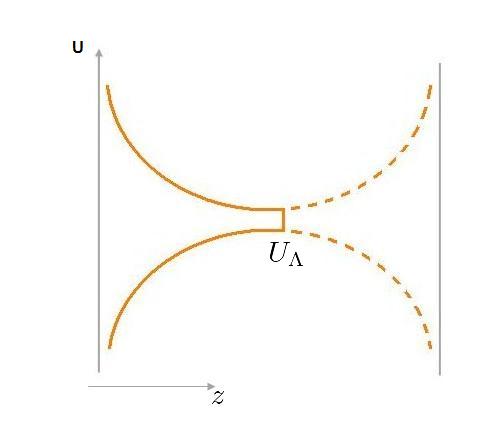
Figure 1: The appearance of a natural infrared cut-off.

Observe that the metric we are dealing with is similar to the metric in the work of Karch and Randall Karch:2000ct . The differences may be summarized as follows.

• In Karch and Randall, they work with

  Lorentzian signature, i.e., $e=-1$,

  the cosmological constant in the braneworld can assume the following values

  AdS, i.e., $\Lambda<0$,

  dS, i.e., $\Lambda>0$;

• In the present work, we shall mainly consider the Euclidean $AdS_{4}$ case given by $e=+1$ with $\Lambda<0$.

III Glueball and Inflaton Spectrum Equation

In this section, we present arguments in favour of a description of the dual of a $0^{++}$ glueball in the inflationary braneworld as an inflaton field.

Although the spacetime we are considering is not asymptotically AdS, it is a conformally compact spacetime. Thus we may systematically use holographic renormalization method. In this setting we may provide some arguments to the claim that the dual to the glueball field is an inflaton field.

Metric (16) may be seen as a simple deformation of the AdS spacetime. One interesting feature of this metric is the appearance of a natural infrared cut-off - see Fig. 1 - depending on the Hubble parameter $H$. Therefore, let’s recap the usual set up in the usual AdS case.

In the gauge theory side, on top of a Minkowski $M_{4}$ spacetime (the boundary of the AdS), we may consider the operator field $\hat{\mathcal{O}}\sim\mathrm{Tr}(F^{2})$. As usual, correlation functions for this operator are obtained by computing the vev of a generating functional formed with the integral on $M_{4}$ of the coupling $\phi_{0}\hat{\mathcal{O}}$, with $\phi_{0}$ seen as a auxiliary field. This auxiliary field is a dual field that may be extended into the bulk of the AdS spacetime as a massless dilaton field.

The holographic renormalization method prescribes that we might obtain the above mentioned correlation functions by working with a renormalized on-shell supergravity action.

Now, instead of considering the Minkowski space above, we consider a $4d$ FRW spacetime in inflationary regime, that is, $H=\dot{a}/a\equiv\textrm{constant}$. As shown in section 2, this space can be embedded into a deformed AdS spacetime. On top of this FRW spacetime, we may consider the same operator field $\hat{\mathcal{O}}\sim\mathrm{Tr}(F^{2})$, and an auxiliary field $\phi_{0}$. Our claim is that $\phi_{0}$ is an inflaton field. We give arguments for this claim below.

Let’s consider the metric as given by (16),

$$\frac{ds^{2}}{R^{2}_{0}\alpha^{\prime}}=\frac{1}{\sin(z)^{2}}\left(dz^{2}+edt^{2}+a_{0}^{2}\delta_{ij}dx^{i}dx^{j}\right).$$ (21)

Therefore, we may rewrite this metric by a proper choice of a defining function. Recall that defining functions are defined up to a scale transformation.

A defining function for the spacetime we are considering is $r(z)=\sin(z)$, as a defining function, i.e., a first order zero at the boundary, $r(0)=0$, with $\partial_{z}r(0)\neq 0$, and $r(z)>0$, for $0<z<\pi$. Furthermore, in the neighbourhood of the boundary $z=0$, we may write $\sin(z)\simeq z$, so that

$$ds^{2}=\frac{1}{z^{2}}\left(dz^{2}+g_{\mu\nu}(t)dx^{\mu}dx^{\mu}\right),$$ (22)

where the $FRW$ metric is obviously smooth as $z\to 0$, so that we may write

$$g_{\mu\nu}(t,z)=g^{(0)}_{\mu\nu}(t)+z\leavevmode\nobreak\ g^{(1)}_{\mu\nu}(t)+z^{2}\leavevmode\nobreak\ g^{(2)}_{\mu\nu}(t)+....$$ (23)

As discussed in Skenderis:2002wp , we may work in a fixed background. That means that we will work in the case where the massless dilaton $\phi$ does not back-react into the space-time. Therefore, we consider the gravitational side action. We consider here a general $D=d+1$ dimension spacetime, where $d$ refers to the braneworld space-time. Recall that we are working in $D=4+1$.

It is now well-known that the fluctuations around massless scalar and gravitational solutions obey formally the same equation of motion of a scalar field coupled to gravity. Thus, to address our studies on glueballs we write down our action below

$$S=\frac{1}{2}\int d^{d+1}x\leavevmode\nobreak\ \sqrt{eg}\leavevmode\nobreak\ \left({{\frac{1}{\kappa_{5}^{2}}(R+\Lambda_{bulk})}}+g^{MN}\partial_{M}\phi\partial_{N}\phi+M^{2}\phi^{2}\right).$$ (24)

The massive scalar term will be removed later for consistence of the conformal dimension of the relevant operator describing glueballs on the dual four-dimensional field theory. The equation of motion for $\phi$ is

$$e\left(\partial_{0}\partial^{0}\phi+(d-1)H_{eff}\partial_{0}\phi\right) + \frac{1}{a_{0}^{2}}\partial_{i}\partial^{i}\phi+$$

$$+U^{1-d}\partial_{z}\left(U^{d-1}\partial^{z}\phi\right) = U^{2}M^{2}\phi.$$ (25)

We set from now on $\partial_{i}\phi=0$, since we want to discuss homogeneous cosmology only. Furthermore, setting $\rho(z)\equiv U(z)^{-2}$, we can look for solution of the form

$$\phi(t,z)=\rho^{\frac{d-\Delta}{2}}\widetilde{\phi}(t,z).$$ (26)

Substituting this ansatz in equation (III), we obtain

$$e\left(\partial_{0}\partial^{0}\widetilde{\phi}+(d-1)H_{eff}\partial_{0}\widetilde{\phi}\right) +$$

$$\partial_{z}\partial^{z}\widetilde{\phi}+\rho^{\prime}\rho^{-1}\left(\frac{d+1}{2}-\Delta\right)\leavevmode\nobreak\ \partial_{z}\widetilde{\phi} +$$

$$\rho^{-1}\left(\rho^{\prime\prime}-\frac{\Delta+1}{2}\leavevmode\nobreak\ \rho^{-1}(\rho^{\prime})^{2}\right)\leavevmode\nobreak\ \left(\frac{d-\Delta}{2}\right)\widetilde{\phi} = M^{2}\leavevmode\nobreak\ \rho^{-1}\widetilde{\phi}.$$ (27)

Now, since $\rho^{-1}\equiv U^{2}\equiv 1/\sin^{2}(z)$, we have

$$\rho^{\prime} = 2\sqrt{\rho-\leavevmode\nobreak\ \rho^{2}}\leavevmode\nobreak\ \leavevmode\nobreak\ \leavevmode\nobreak\ \leavevmode\nobreak\ \textrm{and}$$

$$\rho^{\prime\prime} = 2(1-2\leavevmode\nobreak\ \rho).$$ (28)

Therefore, the equation becomes

$$e\left(\partial_{0}\partial^{0}\widetilde{\phi}+(d-1)H_{eff}\partial_{0}\widetilde{\phi}\right) +$$

$$\partial_{z}\partial^{z}\widetilde{\phi}+\rho^{\prime}\rho^{-1}\left(\frac{d+1}{2}-\Delta\right)\leavevmode\nobreak\ \partial_{z}\widetilde{\phi} +$$

$$(d-\Delta)\leavevmode\nobreak\ \left((\Delta-1)-\Delta\rho^{-1}\right)\widetilde{\phi} = M^{2}\leavevmode\nobreak\ \rho^{-1}\widetilde{\phi}.$$ (29)

Observe that, if we take $H_{eff}\to 0$, then $\rho\to 1/z^{2}$, and the equation becomes

$$e\partial_{0}\partial^{0}\widetilde{\phi}+\partial_{z}\partial^{z}\widetilde{\phi} +$$

$$+2\left(\Delta-\frac{d+1}{2}\right)\leavevmode\nobreak\ \frac{1}{z}\partial_{z}\widetilde{\phi}+\left(\Delta(\Delta-d)-M^{2}\right)\leavevmode\nobreak\ z^{2}\widetilde{\phi} = 0.$$ (30)

This equation can be compared to similar equation obtained in the usual $AdS_{d+1}$ case.

Now, we set $\widetilde{\phi}=T(t)\chi(z)$, so that we can separate equation (III) into

$$e\left(\partial_{0}\partial^{0}T+(d-1)H_{eff}\partial_{0}T\right)-m^{2}T=0,\quad\quad\quad\quad\quad\quad\quad\quad\quad\quad\quad$$ (31)

$$-\partial_{z}\partial^{z}\chi-\left(\frac{d+1}{2}-\Delta\right)\frac{\rho^{\prime}\partial_{z}\chi}{\rho}+\left(M^{2}-\Delta(\Delta-d)\right)\frac{\chi}{\rho}=\left(m^{2}-\leavevmode\nobreak\ (\Delta-d)(\Delta-1)\right)\chi$$ (32)

In the equation for $\chi(z)$, we can consider the Ansatz

$$\chi(z)=\rho^{\alpha}\leavevmode\nobreak\ \psi(z),$$ (33)

so that this equation becomes

$$-\partial_{z}\partial^{z}\psi+\left(\Delta-\frac{d+1}{2}-2\alpha\right)\frac{\rho^{\prime}}{\rho}\partial_{z}\psi +$$

$$\left[\left(\Delta-\frac{d+1}{2}-(\alpha-1)\right)\frac{(\rho^{\prime})^{2}}{\rho^{2}}+\frac{\rho^{\prime\prime}}{\rho}\right. +$$

$$+\left.\left(M^{2}-\Delta(\Delta-d)\right)\frac{1}{\rho}\right]\psi =$$ (34)

$$= \left(m^{2}-(\Delta-d)(\Delta-1)\right)\psi.$$

This equation can be simplified into

$$-\partial_{z}\partial^{z}\psi+\left(\Delta-\frac{d+1}{2}-2\alpha\right)\frac{\rho^{\prime}}{\rho}\partial_{z}\psi +$$

$$+\left(M^{2}-\Delta(\Delta-d)\right)\frac{\psi}{\rho}+2\alpha\left(2\Delta-d-2\alpha\right)\frac{\psi}{\rho} =$$ (35)

$$= \left(m^{2}-(\Delta-d)(\Delta-1)\right)\psi+$$

$$+ \leavevmode\nobreak\ 2\alpha(2\Delta-(d+1)-2\alpha)\leavevmode\nobreak\ \psi$$

We may now set

$$2\alpha=\Delta-\frac{d+1}{2}.$$ (36)

We thus obtain

$$-\partial_{z}\partial^{z}\psi+\left(M^{2}-\Delta(\Delta-d)\right)\frac{\psi}{\rho} +$$

$$+\frac{1}{4}\leavevmode\nobreak\ \left(2\Delta-(d+1)\right)\left(2\Delta-(d-1)\right)\frac{\psi}{\rho} =$$ (37)

$$= \left(m^{2}-(\Delta-d)(\Delta-1)\right)\psi+$$

$$+ \frac{1}{4}\leavevmode\nobreak\ \left(2\Delta-(d+1)\right)^{2}\leavevmode\nobreak\ \psi.$$

Observe that if we set $d=4$, $M=0$ (massless dilaton), which implies $\Delta=4$, then

$$e\left(\partial_{0}\partial^{0}T+3H_{eff}\partial_{0}T\right)-m^{2}T = 0,$$ (38)

$$-\partial_{z}\partial^{z}\psi+\frac{15}{4}\frac{1}{\sin^{2}{z}}\leavevmode\nobreak\ \psi = \left(m^{2}+\frac{9}{4}\right)\leavevmode\nobreak\ \psi.$$ (39)

In conclusion we have obtained an equation for the inflaton field with potential given by $V(T)=\frac{m^{2}}{2}\leavevmode\nobreak\ T^{2}$. This equation is similar to the equation for conservation of energy in a FRW spacetime. Furthermore, the mass $m$ of the inflaton field is quantized according to the equation for $\chi$. This equation gives also the mass spectrum for the glueball. Recall that the final form for the massless dilaton may be written as

$$\phi(t,z)\equiv\rho^{\frac{d-\Delta}{2}}T(t)\chi(z)=\rho^{\frac{d-\Delta}{2}}\rho^{\alpha}T(t)\psi(z)=\left(\sin(z)\right)^{3/4}\leavevmode\nobreak\ T(t)\psi(z).$$ (40)

IV Glueball and Inflaton Spectrum

In this section we obtain the spectrum of the glueball, that is, $m^{2}_{n}$, where $n=1,2,3,...$. For that we have to solve the Schrödinger-like equation

$$-\chi(z)^{\prime\prime}+\frac{V_{0}}{\sin^{2}(z)}\leavevmode\nobreak\ \chi(z)=\left(E+\frac{(d-1)^{2}}{4}\leavevmode\nobreak\ \right)\chi(z)\equiv\tilde{E}\chi(z),$$ (41)

with

$$V_{0} = \frac{d^{2}-1}{4},$$ (42)

$$E\equiv m^{2} = \tilde{E}-\frac{(d-1)^{2}}{4}.$$ (43)

IV.1 Euclidean signature ($e=+1$)

For this case, we set $y=\sin^{2}(z)$

$$\chi(z)=y^{\mu}\leavevmode\nobreak\ \psi(y),$$ (44)

which leads to the hypergeometric equation

$$y(y-1)\leavevmode\nobreak\ \psi(y)^{\prime\prime}+\left((2\mu+\frac{1}{2})-(1+2\mu)y\right)\psi(y)^{\prime}+\left(\frac{E}{4}-\mu^{2}\right)\psi(y)=0,$$ (45)

with

$$\mu=\frac{1}{4}(1+d),$$ (46)

where $\mu$ was chosen to be positive. The solution for this hypergeometric equation is

$$\psi(y)=C_{1}\leavevmode\nobreak\ {}_{2}F_{1}(a,b;c;y)+C_{2}y^{1-c}\leavevmode\nobreak\ _{2}F_{1}(a+1-c,b+1-c;2-c;y),$$ (47)

with

$$c = 1+2\mu,$$ (48)

$$a = \mu+\frac{\sqrt{\tilde{E}}}{2},$$ (49)

$$b = \mu-\frac{\sqrt{\tilde{E}}}{2},$$ (50)

and ${}_{2}F_{1}(a,b;c;y)$ is a hypergeometric function. Now, using the (Dirichlet) boundary conditions

$$\chi(y=0)=0\leavevmode\nobreak\ \hskip 28.45274pt\leavevmode\nobreak\ \chi(y=1)=0,$$ (51)

we have that $C_{2}=0$, and the solution

$$\chi_{n}(y)=\mathcal{N}_{n}\leavevmode\nobreak\ y^{\mu}\leavevmode\nobreak\ _{2}F_{1}(a,b;c;y),$$ (52)

where $a=2\mu-n$, $b=-n$, with $n\in\mathbb{N}$, and $\mathcal{N}_{n}$ is a normalization factor, so that

$$\tilde{E}_{n}=4\leavevmode\nobreak\ (\mu+n)^{2}.$$ (53)

Therefore,

$$m^{2}_{n}=\left(4(\mu+n)^{2}-\frac{(d-1)^{2}}{4}\right)=\frac{1}{4}\leavevmode\nobreak\ \left((1+d+4n)^{2}-(d-1)^{2}\right),$$ (54)

for $n=0,1,2,...$. By relabelling $n\to\frac{n-1}{2}$, the mass spectrum becomes

$$m^{2}_{n}=n(n+d-1).$$ (55)

In the case $d=4$, we obtain Karch:2001cw ; Karch:2000ct

$$m^{2}_{n}=n(n+3),$$ (56)

for $n=1,2,3,...$.

IV.2 Lorentzian signature ($e=-1$)

In this case, it is well-know that there are only a finite number of bound states for the potential. Furthermore there are scattered states, which is not there in the previous $e=+1$ case. We shall be back to this case in the last part of the paper.

V Slow-Roll and It’s Consequences

In this section, we analyse some consequences imposed by the requirement of slow-roll condition. The slow-roll condition is considered in order that the Universe goes through a nearly exponential expansion during an Euclidean time $\tau\sim 1/H^{E}_{eff}$. This condition is obtained by requiring that $\partial_{0}\partial^{0}T_{n}(\tau)=0$, that is, the acceleration term in the equation

$$\left(\partial_{0}\partial^{0}T_{n}+(d-1)H^{E}_{eff}\partial_{0}T_{n}\right)-m_{n}^{2}T_{n}=0$$ (57)

is negligible. Since we shall focus on the transition between two particular inflaton states we do not assume a priori a multi-inflaton cosmology. Thus our slow-roll analysis is based on the equation for an inflaton field $T_{n}$ and the induced Friedman equation Binetruy:1999hy ; Bazeia:2007vx given by its Euclidean form

$${(H^{E}_{eff})}^{2} = -\frac{2}{3}\rho\left(1+\frac{\rho}{2\sigma}\right)=-\frac{2}{3}\rho,\qquad\mbox{for heavy brane, $\sigma\gg 1$}$$ (58)

$$= -\frac{2}{3}\left(\frac{1}{2}\dot{T_{n}}^{2}+V(T_{n})\right)\simeq-\frac{2}{3}V(T_{n}).$$

Notice that the potential has the right sign, $V(T_{n})<0$, in Euclidean time as we can check from equation (57). Below we study the slow-roll conditions for such potential.

This slow-roll condition can be translated into two conditions for the potential $V(T_{n})=-\frac{1}{2}m_{n}^{2}T_{n}^{2}$ and its derivatives as

$$\epsilon\equiv\frac{1}{2}\leavevmode\nobreak\ \left(\frac{V^{\prime}(T_{n})}{V(T_{n})}\right)^{2} \ll 1$$ (59)

$$\eta\equiv\frac{1}{d-1}\leavevmode\nobreak\ \frac{V^{\prime\prime}(T_{n})}{V(T_{n})} \ll 1.$$ (60)

Now, that is possible if the condition

$$-V(T_{n})^{\prime\prime}\ll(d-1)^{2}H_{eff}^{2}\leavevmode\nobreak\ \hskip 5.69046pt\leavevmode\nobreak\ \textrm{i.e.}\leavevmode\nobreak\ \leavevmode\nobreak\ \leavevmode\nobreak\ \left(\frac{m}{(d-1)H_{eff}}\right)^{2}\ll 1.$$ (61)

Thus, in this case, the Friedman equation (58) and the inflaton equation (57) lead to the well-known solution in the the slow-roll regime

$$a_{0}(\tau) = a_{0}\exp{[m_{n}C(T^{0}_{n}\tau+\frac{1}{2}Bm_{n}\tau^{2})]},$$ (62)

$$T_{n}(\tau) = T^{0}_{n}+Bm_{n}\tau,$$ (63)

where $B$ and $C$ are dimensionless constants. The inflationary regime with an exponential ($H^{E}_{eff}\equiv\frac{\dot{a}_{0}}{a_{0}}=const.$) fast growth is valid as long as the masses $m_{n}^{2}\ll 1$. This is also endowed with the fact that the Euclidean time $\tau\equiv\beta=1/T$, so that at high temperature (in beginning of the inflation) this term is subleading. On the other hand, the inflation never ends because the quadratic term in $a_{0}(\tau)$ starts to dominate for later Euclidean times. So from now on, when we will mention ‘end of inflation’ we will mean the end of the exponential inflation.

Let’s now implement the condition for slow-roll inflation into the mass spectrum of the fluctuation. Recalling that the inflaton and the fluctuation have to have the same mass spectrum $m_{n}^{2}$. Therefore

$$m_{n}^{2}=n(n+d-1).$$ (64)

We now replace this condition into the slow-roll condition (61),

$$\frac{m_{n}^{2}}{(d-1)^{2}{(H^{E}_{eff})}^{2}}=\frac{n(n+d-1)}{(d-1)^{2}}\leavevmode\nobreak\ \frac{1}{{(H^{E}_{eff})}^{2}}.$$ (65)

we obtain

$$\frac{m_{n}^{2}}{(d-1)^{2}H_{E}^{2}}\equiv\frac{n(n+d-1)}{(d-1)^{2}}\frac{1}{{(H^{E}_{eff})}^{2}}\ll 1,$$ (66)

substituting $H^{E}_{eff}=\sqrt{\sigma/(d-1)}$, so that

$$n(n+d-1)\ll(d-1)\leavevmode\nobreak\ \sigma.$$ (67)

Now, since $n=1,2,3,...$, we have to solve the following system of inequalities

$$n > 0,$$ (68)

$$n^{2}+(d-1)n-(d-1)^{2}\leavevmode\nobreak\ {(H^{E}_{eff})}^{2} \ll 1.$$ (69)

V.1 The transition between states of inflation and the e-folds number

Let us first consider the e-folds for a transition in between the states $j\to k$, where the inflaton does not roll but rather suffer mass transitions $m_{j}\to m_{k}$ whereas its initial value are $T^{0}_{j}$ and $T^{0}_{k}$. We one can estimate the time interval of such a transition as

$$\Delta\tau\sim\frac{2\pi}{m_{k}-m_{j}}=\frac{2\pi}{\sqrt{k(k+3)}-\sqrt{j(j+3)}}.$$ (70)

Recall that $m_{n}^{2}=n(n+3)$. As we have previously discussed the exponential inflationary regime takes place for very small inflaton masses that we assume to be the ground state ($j=1$) and the end of such an inflation starts for a very large ‘final’ mass, i.e., $k=n_{f}\gg 1$, which of course implies $m_{f}\gg m_{i}$. Thus, we have now the simpler equation for the transition time inflation

$$\Delta\tau\sim\frac{2\pi}{n_{f}}.$$ (71)

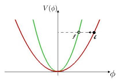
Figure 2: Transition betwen masses $m_{i}$ $\rightarrow$ $m_{f}$. Notice that in the Euclidean case we should consider $-V$.

Now we are ready to estimate the number of e-folds as given by the following equations

$$N_{e} = \int_{\tau_{j}}^{\tau_{k}}{H^{E}_{eff}d\tau}\simeq H^{E}_{eff}\Delta\tau$$ (72)

$$= \frac{2\pi}{n_{f}}\leavevmode\nobreak\ H^{E}_{eff}=\frac{2\pi}{m_{f}}H^{E}_{eff}.$$

One may find from the above relations the most useful relation as being that gives the heaviest inflaton/glueball mass in terms of the e-fold number and the Hubble constant

$$m_{f}=\frac{2\pi H^{E}_{eff}}{N_{e}}.$$ (73)

Notice $({H^{E}_{eff}})^{2}\sim-V(T_{n})$ during the inflation, with $V=-\frac{1}{2}m^{2}_{i}{T^{0}_{i}}^{2}=-\frac{1}{2}m^{2}_{f}{T^{0}_{f}}^{2}$. Now substituting $V$ in terms of initial quantities we find

$$\frac{m_{f}}{m_{i}}\sim\frac{2\pi}{N_{e}}\frac{T_{i}^{0}}{m_{Pl}}.$$ (74)

Note that for the usually assumed initial condition $T_{i}^{0}\sim m_{Pl}$ one finds that for $m_{f}\gg m_{i}$ one needs $N_{e}\to 0$. Thus in the aforementioned transition no inflation really occurs.

Alternatively, one can also understand the previous analysis comparing two inflationary scenarios with distinct rolling inflaton solutions $T_{i}$ and $T_{j}$ given in Eq. (63). Assuming they start and end with the conditions $T_{i}^{0}(\tau_{0})=T_{j}^{0}(\tau_{0})=T_{0}$ and $T_{i}^{f}(\tau^{i}_{f})=T_{j}^{f}(\tau^{j}_{f})=T^{f}$ one can find the final evolution times

$$\tau_{f}^{i}\sim\frac{T^{f}-T_{0}}{m_{i}},\qquad\tau_{f}^{j}\sim\frac{T^{f}-T_{0}}{m_{j}}.$$ (75)

The respectively e-fold numbers can be found as follows

$$N_{e}^{i}=\int_{\tau_{i}=0}^{\tau_{f}^{i}}Hd\tau=H\tau_{f}^{i}\sim\frac{H(T^{f}-T_{0})}{m_{i}},\qquad N_{e}^{j}=\int_{\tau_{i}=0}^{\tau_{f}^{j}}Hd\tau=H\tau_{f}^{j}\sim\frac{H(T^{f}-T_{0})}{m_{j}},$$ (76)

from what follows the ratio

$$\frac{N_{e}^{i}}{N_{e}^{j}}=\frac{m_{j}}{m_{i}}.$$ (77)

Recall that $i<j$. Suppose $i=1$ and the e-folds number is that usually accepted in inflationary cosmology, say $N_{e}^{1}=60$, then

$${N_{e}^{j}}=60\frac{m_{1}}{m_{j}}.$$ (78)

Notice that from this formula it is clear that for any other inflationary scenario other than $j=1$ the e-folds number $N_{e}^{j}$ decreases since $m_{j}>m_{1}$ for $j\neq 1$. In the state with heaviest mass $m_{j}\to\infty$ of course $N_{e}^{j}\to 0$ and the Universe never inflates. On another perspective one can think of that a Universe populated with large glueball masses cannot inflate, but if it decays into lower glueball states it starts to inflate.

Thus, we should focus only on the slow-roll of the lowest state of inflation. The inflaton is then slow-rolling with a determined state with mass $m_{n}$ that according to the previous discussions should be the one with smallest mass $m_{1}$ such that one achieves sufficient inflation. Before ending this subsection some interesting comments are in order. The theory we start with is a pure scalar theory coupled to five-dimensional gravity given in Eq. (24). For absence of dilaton masses ($M=0$) there is no chance of appearing inflation in $d=5$. However, in the four-dimensional theory one has the inflaton fields describing glueballs which may produce sufficient inflation for sufficient small mass (i.e., for the ‘easiest’ four-dimensional scalar potential). Such a dimensional reduction was made by considering a deformed $AdS_{5}$ with time-independent fifth dimension. This certainly is not the case as one uses general Kaluza-Klein compactifications. As it was shown in gibbons ; nunez a theory with no inflation in higher dimensions cannot generate lower dimensional theories with inflation by simple Kaluza-Klein reductions. The first exception was shown in Townsend:2003fx as one considers time-dependent internal coordinates on a manifold with negative cosmological constant.

V.2 The slow-roll in $d=4$ versus entropy in $d=5$ dimensions

In this subsection let us first discuss the e-folds number formula obtained in the slow-roll regime of the the four-dimensional Euclidean cosmology previously discussed. In this case the e-folds number reads

$$N_{e} = \int_{\tau_{j}}^{\tau_{k}}{H^{E}_{eff}d\tau}\simeq H^{E}_{eff}\Delta\tau=H^{E}_{eff}\Delta\beta=H^{E}_{eff}\left(\frac{1}{T_{k}}-\frac{1}{T_{j}}\right)$$ (79)

$$= H^{E}_{eff}\left(\frac{T_{j}-T_{k}}{T_{j}T_{k}}\right)\to dN_{e}=H^{E}_{eff}\frac{dT}{T^{2}},$$

where in the last step we have assumed the temperatures $T_{i}\sim T_{k}\sim T$ and $H^{E}_{eff}\sim const.$ Now we assume $dU=dT$ (from the equipartition theorem) and $dS=dU/T$ (from the thermodynamics second law) to write

$$dN_{e}=\frac{H^{E}_{eff}}{T}\frac{dU}{T}=\frac{H^{E}_{eff}}{T}dS=\frac{H^{E}_{eff}}{T}Vds.$$ (80)

Notice that $s\equiv S/V$ is the entropy density and for relativistic particles goes like $s\sim T^{3}$. $V\sim a(\tau)^{3}$ is the comoving volume element. Conservation of $S$ implies that $s\propto a(\tau)^{-3}$, such that $V\propto s^{-1}$. Also, since $S\equiv sV=const.$ implies that $a(\tau)\sim 1/T=\beta=\tau$, thus as a consequence $H^{E}_{eff}\equiv\frac{\dot{a}(\tau)}{a(\tau)}\sim T$.

Now applying these considerations into our previous formula we find the interesting relationship between entropy density and e-folds number

$$dN_{e}=\frac{ds}{s}\to N_{e}=\ln{s}.$$ (81)

In the following we deal with an interesting similar relationship between the e-folds number and dual black-hole entropy formulas in five dimensions. This is so because the the slow-roll mechanism may be applied in both temporal and spatial coordinates in the suitable dimension. The black-hole entropy formula we mean here stands for that one considered recently in Ref. gubser in the context of equation of state of QCD via dual black-hole solutions in $d=5$ gravity coupled to a scalar field. We should emphasize that we have no black holes in our set up but the deformed Euclidean $AdS$ has an apparent horizon that works as well as in the black hole case.

In this last part we shall be considering the Lorentzian signature ($e=-1$). Notice that the equations of motion (31) and (32) can be rewritten as

$$\ddot{T}+3H\,\dot{T}+V_{T}=0,\qquad V(T)=\frac{1}{2}m^{2}T^{2},$$ (82)

$$\chi^{\prime\prime}+3\frac{U^{\prime}}{U}\chi^{\prime}+V_{\chi}=0,\qquad V(\chi)=\frac{1}{2}m^{2}\chi^{2},$$ (83)

where we have considered $\Delta=d=4$, $e=-1$ and $M=0$. Notice also that $U^{2}=1/\rho$ then follows that $2U^{\prime}/U=-\rho^{\prime}/\rho$. Analogously to the slow-roll regime of $T(t)$ one finds the “slow-varying” $\chi(z)$ such that Eq. (83) is approximated by

$$3\frac{U^{\prime}}{U}\chi^{\prime}+V_{\chi}=0.$$ (84)

Let us now focus on the Einstein equations. The relevant Einstein equations are given by the $0-0$ components

$$-3\left(\frac{\dot{a}_{0}(t)}{a_{0}(t)}\right)^{2}-3e\frac{U^{{}^{\prime\prime}}(z)}{U(z)}+\frac{\Lambda_{bulk}\alpha^{\prime}eU^{2}(z)}{2R_{0}^{2}}=\kappa^{2}_{5}\left(-\frac{1}{2}\dot{\phi}^{\leavevmode\nobreak\ 2}+\frac{e}{2}\phi^{\prime\leavevmode\nobreak\ 2}+\frac{\alpha^{\prime}eU^{2}(z)\leavevmode\nobreak\ M^{2}}{2R_{0}^{2}}\phi^{2}\right),$$ (85)

the $i-i$ components

$$-2e\frac{\ddot{a}_{0}(t)}{a_{0}(t)}-e\left(\frac{\dot{a}_{0}(t)}{a_{0}(t)}\right)^{2} - 3\frac{U^{{}^{\prime\prime}}(z)}{U(z)}+\frac{\Lambda_{bulk}\alpha^{\prime}U^{2}(z)}{2R_{0}^{\leavevmode\nobreak\ 2}}=$$ (86)

$$= \kappa^{2}_{5}\left(\frac{1}{2e}\dot{\phi}^{\leavevmode\nobreak\ 2}+\frac{1}{2}\phi^{\prime\leavevmode\nobreak\ 2}+\frac{\alpha^{\prime}U^{2}(z)M^{2}}{2R_{0}^{2}}\phi^{2}\right),$$

and finally for the $z-z$ components

$$-3e\left(\frac{\dot{a}_{0}(t)}{a_{0}(t)}\right)^{2}-3e\frac{\ddot{a}_{0}(t)}{a_{0}(t)}-6\left(\frac{U^{{}^{\prime}}(z)}{U(z)}\right)^{2} + \frac{\Lambda_{bulk}\alpha^{\prime}U^{\leavevmode\nobreak\ 2}(z)}{2R_{0}^{2}}=$$ (87)

$$\kappa^{2}_{5}\left(\frac{1}{2e}\dot{\phi}^{\leavevmode\nobreak\ 2}-\frac{1}{2}\phi^{\prime\leavevmode\nobreak\ 2}+\frac{\alpha^{\prime}U^{\leavevmode\nobreak\ 2}(z)\leavevmode\nobreak\ M^{2}}{2R_{0}^{2}}\phi^{2}\right),$$

where we have used the metric in the form (11) and the fact that $\phi\equiv\phi(t,z)$, such that $\partial_{i}\phi=0\ (i=1,2,3)$.

There is a vacuum solution satisfying these equations for slow rolling/varying field, i.e. $\dot{\phi}=0,\phi^{\prime}=0$, massless ‘dilaton’ $M=0$ and $\Lambda_{bulk}$ term exponentially suppressed. Such a solution (for $e=-1$) is given by

$$a_{0}(t)=e^{\sqrt{\Lambda}t},\qquad U(z)=e^{-\sqrt{\Lambda}z}.$$ (88)

Let us turn to the slow rolling/varying field regime. We shall consider now the less stringent conditions $\dot{\phi}\simeq 0,\phi^{\prime}\simeq 0$. Recall that $\phi$ describes fluctuations that can be written as $\phi(t,z)=T(t)\chi(z)$. Thus $\dot{\phi}=\dot{T}(t)\chi(z)$ and $\phi^{\prime}=T(t)\chi^{\prime}(z)$. The fields $T(t)$ and $\chi(z)$ are slow rolling/varying consistently if they are given by $T_{n}(t)=T^{0}_{n}-Bm_{n}t$ and $\chi_{n}(z)=\chi^{0}_{n}+Bm_{n}z$, being $m_{n}$ glueball masses. The slow roll regime is ensured as long as $m_{n}\ll 1$ such that we also maintain the conditions $\dot{\phi}\sim m_{n}\chi(z)\simeq 0$ and $\phi^{\prime}\sim m_{n}T(t)\simeq 0$.

Now notice that from $z-z$ component one can readily find (for $e=-1$)

$$3\frac{\ddot{a}_{0}(t)}{a_{0}(t)}+3\left(\frac{\dot{a}_{0}(t)}{a_{0}(t)}\right)^{2}-6\left(\frac{U^{{}^{\prime}}(z)}{U(z)}\right)^{2} = \kappa^{2}_{5}\left(-\frac{1}{2}\dot{\phi}^{\leavevmode\nobreak\ 2}-\frac{1}{2}\phi^{\prime\leavevmode\nobreak\ 2}\right)$$ (89)

$$= \kappa^{2}_{5}B^{2}\left(-\frac{1}{2}m_{n}^{2}\chi^{2}(z)-\frac{1}{2}m_{n}^{2}T^{2}(t)\right).$$

In the slow rolling/varying field regime one the first and second derivative terms have approximately the same value such that one can write the above equation in a simplest form

$$\left(\frac{\dot{a}_{0}(t)}{a_{0}(t)}\right)^{2}-\left(\frac{U^{{}^{\prime}}(z)}{U(z)}\right)^{2}=\frac{\kappa^{2}_{5}B^{2}}{6}\left(-\frac{1}{2}m_{n}^{2}\chi^{2}(z)-\frac{1}{2}m_{n}^{2}T^{2}(t)\right).$$ (90)

This gives us the desired Friedman equation for the spatial component

$$\left(\frac{U^{{}^{\prime}}}{U}\right)^{2}=-\frac{\kappa^{2}_{5}B^{2}}{6}\left(-\frac{1}{2}m_{n}^{2}\chi^{2}(z)-\frac{1}{2}m_{n}^{2}T^{2}(t)-\frac{6H^{2}}{\kappa^{2}_{5}B^{2}}\right)=-\frac{\kappa^{2}_{5}B^{2}}{6}V(\chi),$$ (91)

being

$$V(\chi)=-\frac{1}{2}m_{n}^{2}\chi^{2}-\frac{6H^{2}}{\kappa^{2}_{5}B^{2}},$$ (92)

where we have made $m_{n}^{2}T^{2}(t)$ negligible for $a(t)=\exp{(Ht)}$, being $H\sim const.$. Notice this potential has the property of having a local maximum around $\chi=0$ just as those required in gubser .

Now we are ready to compute the entropy density and the temperature in terms of this potential

$$\ln{s}\equiv N_{e}=\int{dz\frac{U^{\prime}}{U}}=-\int_{\chi_{0}}^{\chi_{H}}{{d\chi}\frac{V(\chi)}{V^{\prime}(\chi)}},$$

$$\ln{T}=\int_{\chi_{0}}^{\chi_{H}}{{d\chi}\left(\frac{1}{2}\frac{V^{\prime}(\chi)}{V(\chi)}-\frac{1}{3}\frac{V(\chi)}{V^{\prime}(\chi)}\right)},$$ (93)

where $\chi_{H}$ is $\chi$ at horizon. We are now able to find equation of state by using such formulas. The sound speed can be readily found in the form

$$c_{s}^{2} \approx \frac{1}{3}-\frac{1}{2}\frac{V^{\prime}(\chi_{H})^{2}}{V(\chi_{H})^{2}}$$ (94)

$$= \frac{1}{3}-\frac{1}{2}\frac{(m_{n}^{2}\chi_{H})^{2}}{(\frac{1}{2}m_{n}^{2}\chi_{H}^{2}+\frac{6H^{2}}{\kappa^{2}_{5}B^{2}})^{2}}.$$ (95)

One can easily find $\chi_{H}$ in terms of the temperature from the temperature formula in (93) for $\chi_{H}\to 0$. In doing this gives $\chi_{H}\sim{T^{-3/m_{n}^{2}}}$. The behavior of the quadratic sound speed $c_{s}^{2}$(up to fourth order in $\chi_{H}$) as a function of the temperature is depicted in Fig. 3.

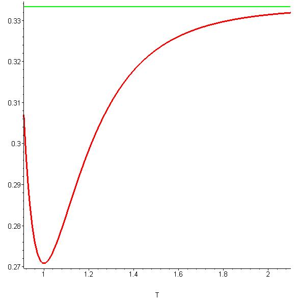
Figure 3: The behavior of the sound speed as a function of the temperature (red) and the its asymptotic value 1/3 (green).

Acknowledgments

The authors are supported in part by CNPq and PROCAD/PNPD-CAPES.

References

(1)
J. M. Maldacena,
Adv. Theor. Math. Phys. 2, 231 (1998)
[Int. J. Theor. Phys. 38, 1113 (1999)]
[arXiv:hep-th/9711200].
(2)
S. S. Gubser, I. R. Klebanov and A. M. Polyakov,
Phys. Lett. B 428, 105 (1998)
[arXiv:hep-th/9802109].
(3)
E. Witten,
JHEP 9812, 012 (1998)
[arXiv:hep-th/9812012].
(4)
C. Csaki, H. Ooguri, Y. Oz and J. Terning,
JHEP 9901, 017 (1999)
[arXiv:hep-th/9806021].
(5)
A. Karch and L. Randall,
Phys. Rev. Lett. 87, 061601 (2001)
[arXiv:hep-th/0105108].
(6)
A. Karch and L. Randall,
JHEP 0105, 008 (2001)
[arXiv:hep-th/0011156].
(7)
P. Binetruy, C. Deffayet, U. Ellwanger and D. Langlois,
Phys. Lett. B 477, 285 (2000)
[arXiv:hep-th/9910219].
(8)
D. Bazeia, F. A. Brito and F. G. Costa,
Phys. Lett. B 661, 179 (2008)
[arXiv:0707.0680 [hep-th]].
(9)
K. Skenderis,
Class. Quant. Grav. 19, 5849 (2002)
[arXiv:hep-th/0209067].
(10) G.W. Gibbons, “Aspects of supergravity theories in Supersymmetry,
Supergravity and Related Topics”, edited by F.
de Aguila, J.A. de Azcárraga and L. Ibañez, 346 (World
Scientific, Singapore, 1985).
(11)
J. M. Maldacena and C. Nunez,
Int. J. Mod. Phys. A 16, 822 (2001)
[arXiv:hep-th/0007018].
(12)
P. K. Townsend and M. N. R. Wohlfarth,
Phys. Rev. Lett. 91, 061302 (2003)
[arXiv:hep-th/0303097].
(13)
S. S. Gubser and A. Nellore,
Phys. Rev. D 78, 086007 (2008)
[arXiv:0804.0434 [hep-th]].