Dynamical Decoupling of Qubits in Spin Bath under Periodic Quantum Control

Abstract

We investigate the feasibility for the preservation of coherence and entanglement of one and two spin qubits coupled to an interacting quantum spin-1/2 chain within the dynamical decoupling (DD) scheme. The performance is examined by counting number of computing pulses that can be applied periodically with period of $T$ before qubits become decoherent, while identical decoupling pulse sequence is applied within each cycle. By considering pulses with mixed directions and finite width controlled by magnetic fields, it is shown that pulse-width accumulation degrades the performance of sequences with larger number of pulses and feasible magnetic fields in practice restrict the consideration to sequences with number of decoupling pulses being less than 10 within each cycle. Furthermore, within each cycle $T$, exact nontrivial pulse sequences are found for the first time to suppress the qubit-bath coupling to $O(T^{N+1})$ progressively with minimum number of pulses being $4,7,12$ for $N=1,2,3$. These sequences, when applied to all qubits, are shown to preserve both the entanglement and coherence. Based on time-dependent density matrix renormalization, our numerical results show that for modest magnetic fields (10-40 Tesla) available in laboratories, the overall performance is optimized when number of pulses in each cycle is 4 or 7 with pulse directions be alternating between x and z. Our results provide useful guides for the preservation of coherence and entanglement of spin qubits in solid state.

I Introduction

The dream of building quantum computers has driven intensive investigations on quantum information processing during the past decade. Nonetheless, due to the ubiquitous decoherence problem, the progress made so far has been limited. Since the processing of a real quantum system includes inevitable disturbance from the outside world, the central challenge is to find ways to control or even eliminate the decoherence. There are different strategies proposed to overcome decoherence such as dynamical decoupling (DD) Lloyd1 ; Lloyd2 ; Viola ; Lidar1 ; Lidar2 ; Das ; Uhrig , quantum error correctionShor ; Steane ; Knill , and decoherence-free subspaceZanardi ; Lidar ; Facchi1 ; Facchi2 . While different strategies have their own advantages, the dynamical decoupling represents the oldest effort along this direction and have been known as a mature technique employed in Nuclear Magnetic Resonance (NMR) experiments. Theoretically, it has been rigorously shown that DD provides upper bounds for error of reduced density matrix caused by quantum evolutionLidar2 . Recent NMR experiments further indicate that dynamical decoupling does preserve coherence of a nuclear-spin qubitLidar5 . These facts clearly indicate that DD is promising in providing a practical solution to defeating decoherence.

To implement the scheme of dynamical decoupling, explicit pulse sequence has to be constructed. Various pulse sequences were proposed and developed. Hanh’s spin echo (SE)Hahn and Carr-Purcell-Meiboom-Gill (CPMG)CPMG were brought up in the beginning. Later, concatenated dynamical decoupling (CDD)Das sequence and Uhrig’s dynamical decoupling (UDD)Uhrig sequence were proposed. With so many pulse sequences available, one still needs to address the central issue in the scheme of dynamical decoupling: what is the sequence that has the best performance in suppressing decoherence while viable quantum manipulations are kept? The issue has been addressed by considering a given cycle of $T$ in which pulses are applied. The performance is examined by number of pulses needed for suppressing the qubit-bath coupling to the order $O(T^{m})$. When durations of pulses are ignored, it was recently shown by Yang and LiuLiu that for a single qubit interacting with bath with Ising-like coupling, the UDD-N pulse sequence can suppress the pure dephasing to $O(T^{N+1})$. However in addition to the control of dephasing, one also needs to control longitudinal relaxation. This would be necessary when the coupling between the qubit and the spin bath is Heisenberg-like. In this case, Yang and LiuLiu showed that the UDD-N pulse sequence can not eliminate the longitudinal relaxation and the dephasing to $O(T^{N+1})$ at the same time. This calls for a closer examination on the minimum number of pulses for suppressing the qubit-bath coupling to the desired order $O(T^{N+1})$. Recently, a quadratic DD sequence (QDD) that concatenating x-direction and z-direction UDD sequences is proposedLidar3 . Although QDD is shown to suppress general decoherence to $O(T^{N+1})$ by using $(N+1)^{2}$ pulse intervals, the sequence is not optimal and the issue of finding the optimal sequence still remains.

From theoretical point of view, if the qubit-bath coupling is the only Hamiltonian that governs qubits, the reduced density matrix $\rho_{r}(T)$ of qubits includes all undesired dynamics. Therefore, for a given $T$ and order $N$, a sequence is optimal if it suppresses all operators in $\rho_{r}(T)$ to $O(T^{N+1})$. However, in order to perform computing, one also needs a strategy for inserting computing pulsesLloyd3 . It is clear that if the suppression due to DD pulses is indiscriminating, the desired dynamics due to computing will also be suppressed unless computing pulses form another commuting DD-pulse sequence. In this case, one decomposes DD pulses into cycles separating by computing pulses. The performance of DD pulses is then examined by number of computing pulses that can be applied before the system becomes decoherent. In addition to the issue of how to insert computing pulses, the finite duration of pulses also represents an important constraint. The accumulation of pulse-width is seen to degrade the performance of DD pulsesLidar5 . It is therefore important to compare performance of sequences with different orders. So far, most construction of DD pulses focuses on single qubit. It is known that the entanglement is particularly important for characterizing the quantum state of multi-qubits and plays the crucial role in quantum information processing. There have been a few investigations of effects of DD pulses on multiqubits. West et al. investigated fidelity of quantum states of four nuclear spin-qubits in the decoherence free spaceLidar5 and found DD does preserve the fidelity. There have also been studies based on pulse control of the entanglement for two qubits in rather simplified models Abliz ; Rao ; Masaki ; Shan . Nonetheless, it is still not clear what would be an optimized sequence for preserving the entanglement.

In this paper, we investigate the feasibility for preservation of decoherence and entanglement of spin qubits within the DD scheme in solid state system. One or two spin qubits coupled to an interacting quantum spin-1/2 chain are considered. We shall examine different strategies for inserting computing pulses within each cycle and demonstrate that computing after decoupling performs the best. We then examine the feasibility by inserting computing pulses periodically with period $T$ within which the same dynamical decoupling pulses are applied. It is shown that error induced by pulse-width accumulation restricts the consideration to sequences with number of pulses being less than $10$ within each cycle. Furthermore, within each cycle $T$, exact nontrivial pulse sequences can be constructed to suppress the qubit-bath coupling to $O(T^{N+1})$ progressively with number of pulses being $4,7,12$ for $N=1,2,3$. Based on time-dependent density matrix renormalization (t-DMRG), our numerical results show that for modest magnetic fields (10-40 Tesla) available in laboratories, the overall performance is optimized when number of pulses in each cycle is 4 or 7 with pulse directions be alternating between x and z.

This paper is organized as follows. In Sec. II, we present our model Hamiltonian and briefly discuss how to apply t-DMRG to analyze the model Hamiltonian. We shall outline the general framework for calculating the dephasing and longitudinal relaxation. In particular, we point out that for general coupling between the qubit and the bath, the preservation of either coherence or entanglement is determined directly by the evolution operator $U(t)$. In Sec. III, we analyze decoherence and longitudinal relaxation of a single qubit by considering pulses with mixed directions. We will explicitly construct pulse sequences for suppressing lower orders of $U(T)$ up to $O(T^{4})$. Furthermore, different strategies for inserting computing pulses are compared. We find that computing after decoupling performs the best. Therefore, we extend DD over a cycle of $T$ to the periodic scheme in which computing pulses are inserted at $nT$. By considering the finite duration of pulses, we further analyze dynamics defined at $nT$. We show that for available magnetic fields, the number of quantum manipulations can be maximized by using sequence consisting of 4 or 7 pulses. Sec. IV is devoted to investigate the entanglement of two qubits. We shall show that regardless whether two qubits are strongly entangled or non-entangled, the entanglement can be preserved by using the same sequence that suppresses the decoherence of a single qubit. We further show that for general multi-qubits scenario, entanglement can be preserved by applying the same sequence to all qubits if separations between qubits are sufficiently large. In Sec. V, we summarize our results and discuss possible generalization to dynamically decouple multi-qubits from the environment. In Appendix A, we explicitly construct equivalent sequences for $N=2$.

II Theoretical Formulation and General Consideration

We consider a system-bath model which is described by the total Hamiltonian $H_{0}=H_{sys}+H_{bath}+H_{int}$, where $H_{sys}$ is the Hamiltonian of a single or two qubits system, $H_{bath}$ is the Hamiltonian of a spin bath and $H_{int}$ represents the interaction between qubits and the bath. The system Hamiltonian $H_{sys}$ is generally zero unless computing pulses or decoupling pulses are applied. Generally, computing pulses can be also spread over all timesLidar5 . In this case, one has

$$\mathcal{H}_{sys}=\vec{s}\cdot\vec{B},$$ (1)

where $\vec{s}$ is the qubit spin operator and $\vec{B}$ is the corresponding magnetic field for computing. The spin bath is a spin chain generally characterized by the $XXZ$ Heisenberg model

$$\mathcal{H}_{bath}=J\sum\left(S^{x}_{i}S^{x}_{i+1}+S^{y}_{i}S^{y}_{i+1}+\Delta S^{z}_{i}S^{z}_{i+1}\right),$$ (2)

where $J>0$. It is known that the XXZ Heisenberg model has a very rich structure.Sachdev2000 The decoherence and entanglement dynamics induced by such kind of spin bath have been recently investigated. rossini:032333 ; Lai In order not to be masked by dynamics of the order parameterHung , we shall focus on the XY regime where $|\Delta|<1$. Since the case of $\Delta\neq 0$ behaves qualitatively the same as $\Delta=0$ case, we shall simply set $\Delta=0$ with understanding that our results are also applicable to $\Delta\neq 0$. Two specific forms of the qubit-bath coupling Hamiltonian $H_{int}$ are considered. In the first scenario we consider Ising-like coupling $H_{int}=\epsilon s^{z}S^{z}_{i}$ for a single qubit or $H_{int}=\epsilon(s_{1}^{z}S^{z}_{i}+s_{2}^{z}S_{j}^{z})$ for two qubits, where $s^{z}(S^{z}_{i})$ is the qubit (spin bath) operators and $i$($j$) is the single site of spin chain to which the qubit is coupled to. It gives rise to pure dephasing of the qubit. To minimize the boundary effect in numerical calculation, $i$($j$) is usually taken to be the central site of the chain. In the second scenario we consider Heisenberg-like coupling $H_{int}=\epsilon\vec{s}\cdot\vec{S}_{i}$ for a single qubit or $H_{int}=\epsilon(\vec{s}_{1}\cdot\vec{S}_{i}+\vec{s}_{2}\cdot\vec{S}_{j})$ for two qubits, which gives rise to both dephasing and energy relaxation.

Figure 1: Illustration of a dynamical decoupling pulse sequence in the periodic decoupling scheme. Here a sequence of pulses, each with width $\tau_{p}$ centered at $t_{k}$, are applied periodically with period $T$. The directions of pulses are alternating and to compensate the even/odd effect of pulse direction, a parity pulse marked by slashed line is applied at the end of the sequence. At $t^{*}=nT$, computing pulses of width $\tau_{o}$ for quantum processing are applied. For convenience, we denote intervals between centers of pulses by $\alpha_{i}T$.

For most of our numerical work, we shall focus on the initial state in which the total state of the system is a product state of the form:

$$|\Phi(0)\rangle=|g\rangle\otimes|G\rangle,$$ (3)

where qubits are in some particular state of interest $|g\rangle$ while the bath is in its ground state $|G\rangle$. Our results, however, are based on the consideration of evolution operator directly. Hence similar results are also found for other initial states.

A pulse sequence in a cycle of $T$ may contain $N$ decoupling pulses centered at $t_{k}$ where $k=1,2,\cdots,N$ as illustrated in Fig. 1. Because number of pulses along the same direction may not be even, to compensate this parity effect, a parity pulse is added at the end of the sequence. We shall denoted intervals between $t_{k}$ by $\alpha_{i}T$. Typically in an experiment, these pulses are generated by a magnetic field $B(t)\hat{n}$ and have the same width $\tau_{p}$ . We concentrate on the pulse sequences in which each pulse gives rise to a $\pi$ rotation along a given control axis $\hat{n}$ for some qubit. If pulses are characterized by a time-dependent control Hamiltonian $H_{c}(t)$, the total system is then characterized by the Hamiltonian

$$H(t)=H_{c}(t)+H_{0},$$ (4)

with

$$H_{c}(t)=\sum_{i,k}A(t-t_{k})\vec{s}_{i}\cdot\hat{n}^{i}_{k}.$$ (5)

Here $\vec{s}_{i}$ represents the spin of $i^{\rm th}$ qubit and $\hat{n}^{i}_{k}$ is the control axis during the $k^{\rm th}$ pulse that is applied at the $i^{\rm th}$ qubit. $A(t-t_{k})$ is a square function centered at $t_{k}$ with width $\tau_{p}$. The magnitude of $A$ is $\mu_{b}B$ with $\mu_{b}$ being the Bohr magneton and $B$ be the magnetic field so that $J\tau_{p}=10\pi J({\rm meV})/B({\rm Tesla})$. Experimentally, accessible magnetic field $B$ will impose a lower bound on the pulse duration $\tau_{p}$.

We shall focus on periodic dynamical decoupling where $H_{c}(t+T)=H_{c}(t)$ and $T$ is the period of the pulse sequence. Manipulating or computing pulses with width $\tau_{o}$ are applied at $t^{*}=T,2T,3T,\cdots$. Since both $\tau_{o}$ and $\tau_{p}$ are determined by available magnetic fields, we shall assume $\tau_{o}=\tau_{p}$. Furthermore, in order that pulses are non-overlapping, one requires

$$T>{\rm max}\left[\frac{\tau_{p}}{\alpha_{i}}\right].$$ (6)

Since $\alpha_{i}({\rm min})\leq 1/(N+1)$, we have $T\geq(N+1)\tau_{p}$. Therefore, $T$ depends on $N$. In the following we will denote $T$ by $T_{N}$ to indicate its explicit dependence on $N$. Formally the evolution of the total system is dictated by the evolution operator

$$U(t)=\mathcal{T}e^{-i\int_{0}^{t}H(s)ds},$$ (7)

where we have set $\hbar$ to one and $\mathcal{T}$ is the time-ordering operator. During each pulse period, the evolution operator for the kth pulse can be written as

$$U_{k}\equiv\mathcal{T}exp^{-i\int^{t_{k}+\tau_{p}/2}_{t_{k}-\tau_{p}/2}H(s)ds}$$ (8)

$$= \mathcal{T}e^{-i\int^{t_{k}}_{t_{k}-\tau_{p}/2}H_{0}(s)ds}\mathcal{T}e^{-i\int^{t_{k}+\tau_{p}/2}_{t_{k}-\tau_{p}/2}H_{c}(s)ds}$$

$$\times\mathcal{T}e^{-i\int^{t_{k}+\tau_{p}/2}_{t_{k}}H_{0}(s)ds}e^{O(N\epsilon J\tau^{2}_{p})},$$

where the second equality introduces an error of the order $\tau^{2}_{p}$. Since for each qubit one has $\int^{t_{k}+\tau_{p}/2}_{t_{k}-\tau_{p}/2}H_{c}ds=\pi\vec{s}_{i}\cdot\hat{n}^{i}_{k}$, the evolution operator can be expressed as

$$U^{(N)}(t)=(-i)^{N}e^{-iH_{0}(t-t_{N})}\Pi_{i}\vec{\sigma}_{i}\cdot\hat{n}^{i}_{N}e^{-iH_{0}(t_{N}-t_{N-1})}\times$$

$$\Pi_{i}\vec{\sigma}_{i}\cdot\hat{n}^{i}_{N-1}e^{-iH_{0}(t_{N-1}-t_{N-2})}\Pi_{i}\vec{\sigma}_{i}\cdot\hat{n}^{i}_{N-2}\cdots e^{-iH_{0}t_{1}}\times$$

$$\left[1+O(N\epsilon J\tau^{2}_{p})\right],$$ (9)

where $\vec{\sigma}=2\vec{s}$ are the Pauli matrices for the qubit and the rotational matrix $e^{-i\pi(\vec{s}\cdot{\hat{n}}_{k})}$ is reduced to $i\vec{\sigma}\cdot{\hat{n}}_{k}$. Eq.(9) thus implies that to the order of $\tau^{2}_{p}$, $N$ pulses of finite width can be consider as ideal pulses without width so that qubits are flipped right after $t_{k}$.

In general it is difficult to exactly evaluate $U^{N}(t)$. t-DMRG, however, provides a way to efficiently evolve such a state with high accuracy for a quasi-one dimensional system. We first use static DMRG to find the ground state of the spin chain bath for a given $\Delta$ and then use the method of t-DMRG to evaluate $U^{N}(t)|\Phi(0)\rangle$ numerically. We note that the degrees of freedom of the qubits are kept exactly during the t-DMRG calculation by targeting an appropriate state. The dimension of the truncated Hilbert space is set to be $D=100$. For short time simulation we set $J\delta t=0.005$ in the Trotter slicing while for effective dynamics we set $J\delta t=0.01-0.02$ to balance the Trotter error and truncation error. Similar procedure has recently been used to investigate the decoherence and entanglement dynamics induced by spin bath. We hence refer to Ref.[Lai, ] and the references therein for details of simulation procedure.

From $U(t)$, one obtains the reduced density matrix $\rho_{r}$ of qubits by tracing out the environment

$$\rho_{r}(t) = Tr_{\text{bath}}{\ U(t)\rho(0)U^{\dagger}(t)}$$ (10)

$$= \sum_{E}\langle\Phi_{E}|U(t)\rho(0)U^{\dagger}(t)|\Phi_{E}.\rangle$$

Here $|\Phi_{E}\rangle$ is a complete set of state for the spin chain and $\rho(0)$ is the total density matrix at $t=0$. Since the initial total wavefunction is a product of state, one may consider $\rho(0)=|p\rangle\langle q|\otimes|G\rangle\langle G|$, where $|p\rangle$ ($|q\rangle$) is an eigenstate to the total $s^{z}$ of qubits with the eigenvalue being $p$ ($q$). At time $t$, the reduced density matrix is given by

$$\rho_{r}(t)=\sum_{E}\langle\Phi_{E}|U(t)|p\rangle|G\rangle\langle G|\langle q|U^{\dagger}(t)|\Phi_{E}\rangle.$$ (11)

For Ising-like coupling, $\hat{n}$ will be taken to be $\hat{x}$ so that one can replace $\sigma^{z}$ by $\pm$. Therefore, one has

$$U(t)|\pm\rangle = e^{-i(t-t_{N})(H_{0}\pm(-1)^{N}\epsilon S^{z})}\cdots e^{-i(t_{2}-t_{1})(H_{0}\mp\epsilon S^{z})}$$ (12)

$$\times e^{-it_{1}(H_{0}\pm\epsilon S^{z})}|\pm\rangle$$

$$\equiv U_{\pm}(t)|\pm\rangle.$$

Hence one can replace $U(t)|p\rangle$ by $U_{p}(t)|p\rangle$. We find

$$\rho_{r}(t)=|p\rangle\langle q|\left[\sum_{E}\langle\Phi_{E}|U_{p}(t)|G\rangle\langle G|U^{\dagger}_{q}(t)|\Phi_{E}\rangle\right].$$ (13)

Since $U_{p}(t)$ no longer acts on $|p\rangle$, one can switch the order of $\langle\Phi_{E}|U_{p}(t)|G\rangle$ and $\langle G|U^{\dagger}_{q}(t)|\Phi_{E}\rangle$. Using the completeness of $|\Phi_{E}\rangle$, one obtains

$$\rho_{r}(t)=|p\rangle\langle q|\langle G|U^{\dagger}_{q}(t)U_{p}(t)|G\rangle.$$ (14)

Hence the matrix element of the reduced density matrix is given by

$$\rho^{pq}_{r}(t)=\langle G|U^{\dagger}_{q}(t)U_{p}(t)|G\rangle.$$ (15)

It is clear that the effectiveness of DD control for the Ising-like coupling is determined by $U^{\dagger}_{q}(t)U_{p}(t)$.

On the other hand, if the coupling between the qubit and the spin bath is Heisenberg-like, $|p\rangle$ is no longer an eigenstate to $U(t)$. The reduction from Eq.(10) to Eq.(14) is generally not possible except for the diagonal elementsLiu . Therefore, one resorts to Eq.(10) to calculate the reduced density matrix. In this case, the matrix element of the reduced density matrix is given by

$$\rho^{pq}_{r}(t) = Tr_{\text{bath}}\langle p|U(t)\rho(0)U^{\dagger}(t)|q\rangle$$ (16)

$$= Tr_{\text{bath}}\left[\rho(0)U^{\dagger}(t)|q\rangle\langle p|U(t)\right].$$

In general, $|q\rangle\langle p|$ does not commute with $U(t)$. Hence the effectiveness of bang-bang control for the Heisenberg-like coupling is determined by the evolution operator $U(t)$. Note that for longitudinal component when $p=q=\pm$ for a single qubit, Yang and LiuLiu noticed that for the UDD-N pulse sequence applied at a single qubit, $U(T_{N})=\exp\left[iH_{eff}T_{N}+O(T_{N}^{N+1})\right]$ and $H_{eff}$ commutes with $|+\rangle\langle+|$ and $|-\rangle\langle-|$. As a result, the linear term in $T_{N}$ gets canceled and thus the magnetization $\langle\sigma_{z}(T)\rangle$ can be controlled to $1+O(T_{N}^{N+1})$. Apparently, the same cancelation does not happen for the off-diagonal matrix elements where $H_{eff}$ does not commute with $|p\rangle\langle q|$. Therefore, to find an effective sequence for both dephasing and longitudinal relaxation, one needs to directly control $U(t)$ to the required order.

III Short Time and Long time Dynamics of Single Qubit Decoherence

In this section, we examine dynamics of a single qubit coupled to the spin bath with and without decoupling pulses. For short time dynamics of a qubit under DD pulses within a cycle of $T$, we construct pulse sequences for suppressing lower orders of $U(T)$ up to $O(T^{4})$. Different strategies for inserting computing pulses are compared. By using t-DMRG, we demonstrate that computing after decoupling performs the best. Therefore, we extend DD over a cycle of $T$ to the periodic scheme in which computing pulses are inserted at $nT$. In particular, we shall compare long time dynamics of different sequences at $nT$ to determine the optimized sequence.

III.1 Ising-like coupling

We start by examining the case when the qubit-bath coupling is Ising-like. In this case, there is no longitudinal relaxation since $[s_{z},H]=0$. The pure dephasing is characterized by the Loschmidt echo $L(t)\equiv\mid\rho^{+-}_{r}(t)\mid^{2}$, where $\rho^{+-}_{r}$ is defined by Eq.(15). In the absence of decoupling pulses, it is known that the Loschmidt echo decays as $L(t)=e^{-\alpha t^{2}}$ for short timesLai . Hence $\alpha$ characterizes the short time decoherence of a single qubit in spin bath. When the spin bath is modeled by a XY model(i.e., $\Delta=0$) and $H_{int}=\epsilon s^{z}S^{z}_{i}$, $\alpha$ can be exactly calculated and will be served as a checking point of our t-DMRG numerical code. To find $\alpha$, we first note that after the Wigner-Jordan transformation, the Hamiltonian is quadratic and is given by $H_{0}=J\sum_{n}c^{\dagger}_{n}c_{n+1}+h.c.+\epsilon s_{z}c^{\dagger}_{i}c_{i}$ . As a result, $L(t)$ can be expressed as Rossini

$$L(t)=\mid\mathrm{det[1+r(e^{itH^{-}}e^{-itH^{+}}-1)]\mid^{2}.}$$ (17)

Here $H^{\pm}$ are the matrices corresponding to $H_{0}$ with $s_{z}=\pm 1$. $r$ is a $2N\times 2N$ matrix with N is the length of the spin chain and its element is given by $r_{ij}=\langle c^{\dagger}_{i}c_{j}\rangle$. By using the identity for the operator $\hat{A}$

$$\det\left[1+\hat{A}\right] = e^{Tr\ln\left(1+\hat{A}\right)}$$ (18)

$$= e^{Tr\hat{A}-Tr\hat{A}^{2}/2+\cdots}$$

and expanding $e^{itH^{\pm}}=1+itH^{\pm}-t^{2}(H^{\pm})^{2}/2\cdots$, one find $\alpha=\epsilon^{2}$.

On the other hand, in the presence of N decoupling pulses in a period $T_{N}$, it has been shown that the UDD-N pulse sequence suppressesLiu $U_{-}^{\dagger(N)}(T_{N})U^{(N)}_{+}(T_{N})=1+O(T_{N}^{N+1})$ and the effectiveness increases as $N$ increases. As a check, in Fig.2, we show our numerical simulations of $L(T)$ versus $T$ using t-DMRG. For the free decay without decoupling pulses, fitting within $0<Jt<0.1$, we find that $\alpha=0.0224$ for $J=1$ and $\epsilon=-0.15$. This is in agreement with the analytic result $0.0225$ within the error caused by the Trotter time slicing ($J\delta t=0.005$). We also observe that higher order UDD pulse sequence is more effective as expected.

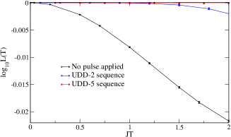
Figure 2: (Color online) Numerical simulations of Loschmidt echo $L(T)$ versus $T$ by t-DMRG for Ising-like coupling. Here for a given $T$, all pulses for any pulse sequence are arranged within $T$. The fitted decaying parameter $\alpha$ for the free case is $0.0224$ , in agreement with the analytic result. It is clear that higher order UDD pulse sequences are more effective. Note that in this and the following figures, error bars are given for each data point with figure legends being positioned at the intersection point of the curve with the error bar. In the current figure, errors are about the same sizes of figure legends.

III.2 Short-time behavior of Heisenberg-like coupling

When the coupling of the qubit to the spin bath is Heisenberg-like, $s_{z}$ is no longer a good quantum number. To suppress both longitudinal and transverse relaxations, we consider $N$ $\pi$-pulses with alternating directions along $x$ and $z$ axes in the period of $T_{N}$. The evolution operator then becomes

$$U^{(N)}(t)=(-i)^{N}e^{-iH_{0}(t-t_{N})}\sigma_{x}e^{-iH_{0}(t_{N}-t_{N-1})}\sigma_{z}\times$$

$$\cdots\sigma_{z}e^{-iH_{0}(t_{2}-t_{1})}\sigma_{x}e^{-iH_{0}t_{1}}\left[1+O(N\epsilon J\tau^{2}_{p})\right].$$

(19)

Since for any operator $\hat{O}$, one has

$$\sigma_{\alpha}\hat{O}(\vec{\sigma})\sigma_{\alpha}=\hat{O}(\sigma_{\alpha}\vec{\sigma}\sigma_{\alpha}).$$ (20)

By inserting appropriate identities, $\sigma^{2}_{\alpha}=1$, one can move all the spin operators to the left and obtains

$$U^{(N)}(t) = (-i)^{N}\sigma_{x}\sigma_{z}\cdots\sigma_{z}\sigma_{x}U^{(N)}_{0}\left[1+O(N\epsilon J\tau^{2}_{p})\right]$$ (21)

$$= (-i)^{p}\sigma_{p}U^{(N)}_{0}\left[1+O(N\epsilon J\tau^{2}_{p})\right].$$

Here $p$ is an integer and has no contribution in $\rho_{r}$. $\sigma_{p}$ is a spin operator representing the net operation by $\sigma_{x}\sigma_{z}\cdots\sigma_{z}\sigma_{x}$. For example, when $N=3$, $\sigma_{p}=\sigma_{z}$. It is clear that $\sigma_{p}$ acts as a parity pulse that compensate fast changes due to pulses. To remove its effect, we must add an additional pulse $\sigma_{p}$ at $T$ so that $U^{(N)}(t)=U^{(N)}_{0}(t)$ where $U^{(N)}_{0}$ is the evolution operator for ideal pulses without width and is given by

$$U^{(N)}_{0}(t)=e^{-iH^{R_{\alpha_{N+1}}}_{0}(t-t_{N})}e^{-iH^{R_{\alpha_{N}}}_{0}(t_{N}-t_{N-1})}\times$$

$$\cdots e^{-iH^{R_{3}}_{0}(t_{3}-t_{2})}e^{-iH^{R_{2}}_{0}(t_{2}-t_{1})}e^{-iH^{R_{1}}_{0}t_{1}}.$$ (22)

In this expression the time-dependent effective Hamiltonian is defined as

$$H^{R_{n}}_{0}=H_{bath}+\frac{\epsilon}{2}[f_{x}(t)\sigma_{x}S^{x}_{i}+f_{y}(t)\sigma_{y}S^{y}_{i}+f_{z}(t)\sigma_{z}S^{z}_{i}],$$ (23)

with $f_{\mu}=\pm 1$, $\mu=x,y,z$ depending on the sequence. Consequently,

$$U^{(N)}_{0}(t)=e^{-iH_{bath}t}\times$$

$$\mathcal{T}e^{\left[-i\frac{\epsilon}{2}\int_{0}^{t}f_{x}(s)\sigma_{x}S^{x}(s)+f_{y}(s)\sigma_{y}S^{y}(s)+f_{z}(s)\sigma_{z}S^{z}(s)ds\right]}$$

$$\equiv e^{-iH_{bath}t}G^{N}(t).$$ (24)

Here $f_{x,y,z}(s)$ characterizes the sequence history of signs, while $S^{\mu}(t)$ is the operator $S^{\mu}_{i}$ in the interaction picture:

$$S^{\mu}(t)=e^{iH_{bath}t}S^{\mu}_{i}e^{-iH_{bath}t}$$

$$=\sum^{\infty}_{n=0}\frac{(it)^{n}}{n!}\underbrace{[H_{bath},[H_{bath},\cdots[H_{bath},S^{\mu}_{i}]\cdots]]}_{n{\rm-folds}}$$

$$\equiv\sum^{\infty}_{n=0}S^{\mu}_{n}t^{n}.$$ (25)

It is clear that since $H_{bath}$ commutes with the qubit spin, $e^{-iH_{bath}t}$ in Eq.(24) gets canceled in Eq.(16) Hence one only needs to suppress $G^{N}(T)$ to the desired order. For this purpose, we re-express $G^{N}(T)=\exp(\Omega^{N}(T))$ and use the Magnus expansionmagnus $\Omega^{N}(T)=\Omega^{N}_{1}+\Omega^{N}_{2}+\cdots$ to evaluate $G^{N}(T)$, where by setting $A(s)=f_{x}(s)\sigma_{x}S^{x}(s)+f_{y}(s)\sigma_{y}S^{y}(s)+f_{z}(s)\sigma_{z}S^{z}(s)$, one has

$$\Omega^{N}_{1}(T)=\int^{T}_{0}A(s)ds$$ (26)

$$\Omega^{N}_{2}(T)=\frac{1}{2}\int^{T}_{0}ds_{1}\int^{s_{1}}_{0}ds_{2}[A(s_{1}),A(s_{2})].$$ (27)

If we want to suppress the decoherence to $m$-th order we must suppress $U^{(N)}_{0}(T_{N})$ to $O(T_{N}^{m})$, but at the same time due to the finite width of pulses we also need to ensure $O(N\tau^{2}_{p})<O(T_{N}^{m})$. Using Eq.(6), we find the minimum of $T_{N}$ is determined by

$$T_{N} \gtrsim {\rm max}\left[(N+1)\tau_{p},(NJ^{2-m}\tau_{p}^{2})^{1/m}\right]$$ (28)

$$\gtrsim {\rm max}\left[\frac{\tau_{p}}{\alpha_{i}},(NJ^{2-m}\tau_{p}^{2})^{1/m}\right].$$

We note that when $m$ is small, the first term dominates. It is thus sensible to define a minimum period as $T_{c}=\tau_{p}/min(\alpha_{i})$. Another important observation is that due to the finite width of pulses, increasing number of pulses also increase $T_{N}$ which leads to stronger decoherence. To find long-time dynamics at $t^{*}=nT_{N}$, we shall start from $m=1$ and focus on small $m$. For a fixed $m$ we find the minimum number of pulses needed, identify the optimized value of $\alpha_{i}$, and compare the results from different $m$. Indeed, as we shall see, increasing $m$ degrades the long-time dynamics in some cases.

To suppress $G^{N}(T_{N})$ to $O(T_{N}^{m})$, we keep the mth order term in Eqs.(26) and (27). For $m=1$, there are three independent operators, $\sigma_{\mu}S^{\mu}_{i}$ ($\mu=x,y,$ and $z$), whose coefficients have to vanish. We hence obtain three constraints

$$\int^{T_{N}}_{0}f_{\mu}(t)dt=0.$$ (29)

These constraints can also be obtained from a geometric perspective, as pointed out in Ref.chen2006, . Therefore we find that the minimum number of pulses is $N_{1}=4$ (including the parity pulse). Eqs.(29) provide three equations for intervals $\alpha_{i}$ where $i=1,2,3,4$. Together with $\sum_{i}\alpha_{i}=1$, we find that there is only one solution with alternating $x$-$z$, equally spaced pulse sequence

$$\alpha_{1}=\alpha_{2}=\alpha_{3}=\alpha_{4}=\frac{1}{4}.$$ (30)

For $m=2$, there are two additional contributions in Eqs.(26) and (27) to $O(T_{N}^{2})$ in $G^{N}(T_{N})$. By using Eq.(29), terms with double integrals can be rewritten as

$$I_{2}\equiv\int^{T_{N}}_{0}dt_{1}\int^{t_{1}}_{0}d{t_{2}}f_{\mu}(t_{1})f_{\nu}(t_{2})[S^{\mu}(t_{2}),S^{\nu}(t_{1})].$$ (31)

Since $[\sigma_{\mu}S^{\mu}_{i},\sigma_{\nu}S^{\nu}_{i}]=0$, all double integrals vanish and only single integrals contribute. There are three independent operators in Eq.(26). Consequently, in addition to Eqs.(29), we require the 1st moment of $f_{\mu}$ to vanish

$$\int^{T_{N}}_{0}tf_{\mu}(t)dt=0.$$ (32)

By solving Eqs.(29) and (32) for all possible directions of pulses, we find that there are 5 solutions. To continue from the case of $m=1$, we shall adopt the alternating $x$-$z$ pulse sequence and refer the reader to the Appendix for the remaining sequences. Hence, by including the parity pulse ($y$-pulse), the minimum number of pulses for $m=2$ is $N_{2}=7$ with intervals for six pulses being

$$\alpha_{1}=\frac{7-\sqrt{33}}{16}=\alpha_{7},\hskip 5.69046pt\alpha_{2}=\frac{1}{8}=\alpha_{6},$$

$$\alpha_{3}=\frac{\sqrt{33}-3}{16}=\alpha_{5},\hskip 5.69046pt\alpha_{4}=\frac{1}{4}.$$ (33)

Similarly for $m=3$ the second moment of $f_{\mu}$ has to vanish.

$$\int^{T_{N}}_{0}t^{2}f_{\mu}(t)dt=0.$$ (34)

Additionally, there are six mixed moments which have to vanish too

$$\int^{T_{N}}_{0}dt_{1}\int^{t_{1}}_{0}dt_{2}(t_{1}-t_{2})[f_{\mu}(t_{1})f_{\nu}(t_{2})+f_{\mu}(t_{2})f_{\nu}(t_{1})]=0.$$

(35)

Therefore, in general, the minimum number of pulses for $m=3$ is $N_{3}=15$. However, for spin-$1/2$ qubits, since $\sigma^{2}_{\mu}=1$ and $(S^{\mu})^{2}=\hbar^{2}/4$, terms with $\mu=\nu$ in Eq.(35) have no contribution to dynamics of qubits. Therefore, the minimum number of pulses for a spin-$1/2$ qubit is $N_{3}=12$. The equations of $\alpha_{k}$ imposed by Eq.(35) is generally very complicated. Therefor, one has to resort to numerical methods to obtain solutions. By solving Eqs.(29), (32), (34) and (35) for alternating $x$-$z$ pulse sequence, we find the numerical values for intervals are

$$\alpha_{1}\cong 0.0171,\hskip 2.84544pt\alpha_{2}\cong 0.0468,\hskip 2.84544pt\alpha_{3}\cong 0.0658\hskip 2.84544pt\alpha_{4}\cong 0.1013,$$

$$\alpha_{5}\cong 0.1184,\hskip 2.84544pt\alpha_{6}\cong 0.1006\hskip 2.84544pt\alpha_{7}\cong 0.1195,\hskip 2.84544pt\alpha_{8}\cong 0.1049,$$

$$\alpha_{9}\cong 0.0823\hskip 2.84544pt\alpha_{10}=0.1025\hskip 2.84544pt\alpha_{11}\cong 0.0647\hskip 2.84544pt\alpha_{12}\cong 0.0439,$$

$$\alpha_{13}\cong 0.0318.$$ (36)

This is the optimized sequences for suppressing $U(T)$ to $O(T^{4})$. As indicated in the beginning, due to finite width of pulses, $m$-th order (or $O(T^{m})$) sequence is not necessarily more effective than the $(m-1)$-th order (or $O(T^{m-1}))$ sequence. Hence we shall stop at $O(T^{4})$ and compare the performance of different orders at $nT$.

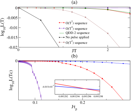
Figure 3: (Color online) (a) Loschmidt echo $L(T)$ versus $T$ of different orders simulated by t-DMRG for Heisenberg-like coupling with $\epsilon=-0.3$. Note that errors are about the same sizes of figure legends. Clearly, $L(T)$ gets improved for increasing number of orders. (b) $L(T_{c})$ versus $J\tau_{p}$. It is seen for as $\tau_{p}$ decreases, $O(T^{3})$ sequence starts to win over $O(T^{2})$ sequence.

In Fig. 3(a), we first show numerical results of $L(t)$ for $0\leq t\leq T$ based on t-DMRG for different sequences with a fixed $T$. This corresponds to the ideal pulse scenario in which the pulse width is neglected. Here we do observe that higher order sequences are more effective. To take the finite width into consideration, in Fig. 3(b) we show numerical results of $L(T_{c})$ versus $J\tau_{p}$ for sequence of different order. One should keep in mind that $T_{c}$ depended on $\tau_{p}$. One can see clearly in Fig. 3(b) that as $\tau_{p}$ decreases, $O(T^{3})$ sequence starts to win over $O(T^{2})$ sequence. We note that for a much smaller $\tau_{p}$ the $O(T^{4})$ sequence will out-perform $O(T^{2})$ and $O(T^{3})$ sequences (not shown in the figure). As a check on if our results depend on the initial state of the spin chain, in Fig. 4, we compare the Loschmit echo versus $T$ by using $|\Phi(0)\rangle=|g\rangle\otimes|bath\rangle$ with the state of bath $|bath\rangle$ being the ground state or the first excited state of the quantum spin chain. One can see that their difference is within the error bar. In addition, we can also form entangled state of the qubit and the bath to check the performance of our sequences. Since after the first cycle $T$, qubit and bath is entangled. Therefore, the performance at later times is an indirect check and this will be done in the next section.

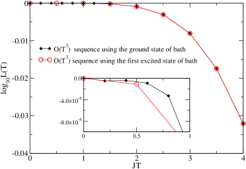
Figure 4: (Color online) Comparison of Loschmit echo by using different initial states. Note that errors are smaller than sizes of figure legends.

In Fig. 5, we compare longitudinal relaxation under UDD-3 and our optimized sequences. It is clear that the optimized sequences outperforms the UDD-3 sequence.

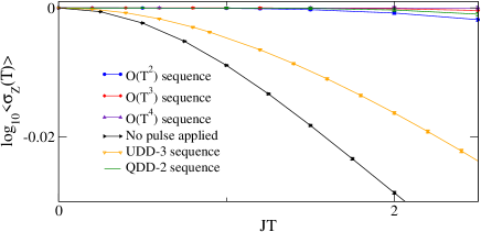
Figure 5: (Color online) Comparison of longitudinal relaxation of different orders with UDD-3 and QDD-2 sequences. Here $\epsilon=-0.3$ and errors are about the same sizes of figure legends.

III.3 Long time dynamics of Heisenberg-like coupling

Given the dynamics of dynamical decoupling, one needs a strategy for inserting the computing pulses. For this purpose, we compare three possible ways to insert a computing pulse that rotates the qubit by an angle $\theta$: (i) using a constant $B$ over $T$ in Eq.(1) (ii) applying a short pulse to rotate the qubit by $\theta$ at some moment $t$ with $0<t<T$ (iii) applying a short pulse at $T$ after all decoupling pulses. From the construction of $O(T^{N})$ sequences, since $H_{sys}$ in Eq.(1) can be combined with $H_{int}$ with $\vec{S}_{i}$ being replaced by $\vec{S}_{i}+\vec{B}$, one expects that computing pulses inserted in $0<t<T$ will be suppressed. In Fig. 6, we show that the distance of $\rho_{r}$ to the desired reduced density matrix versus $\theta$ for three different schemes. Indeed, the results clearly show that DD pulses suppress the computing as well if one adopts the scheme of computing while decoupling. Hence we shall adopt the scheme for inserting computing pulses after decoupling pulses.

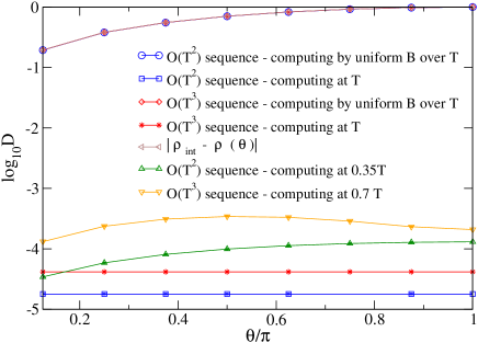
Figure 6: (Color online) Comparison of three differen schemes for inserting a rotation $\theta$. Note that errors are smaller than sizes of figure legends and $B=25$ Tesla so that $O(T^{2})$ sequence outperforms $O(T^{3})$ sequence. Here initially the spin qubit is in the state $|+\rangle$ and $\rho({\theta})$ is the corresponding density matrix by applying a rotation of $\theta$ along $x$-axis on $|+\rangle$ directly. $D=|\rho_{r}-\rho({\theta})|$ is the distance between the simulated reduced matrix and $\rho({\theta})|$ with $|A|=Tr\sqrt{A^{\dagger}A}$

In the following, we shall adopt the scheme that computing pulses are inserted at $nT$ while the same DD pulses are applied between computing pulses. We would like to demonstrate that in this scheme, there will be cross-overs of the relative effectiveness for different sequences. Based on the above optimized sequences within a cycle of $T_{c}$, the performance at $nT_{c}$ can be deduced. Since $U(nT_{c})=U(T_{c})^{n}$, we have

$$U^{(N)}(nT_{c})=\left\{(-i)^{p}U^{(N)}_{0}\left[1+O(N\epsilon J\tau^{2}_{p})\right]\right\}^{n}$$

$$\approx\left\{(-i)^{p}\left[1+O(\epsilon J^{m-1}T^{m})\right]\right\}^{n}$$

$$\approx\left\{(-i)^{p}\right\}^{n}\left[1+O(n\epsilon J^{m-1}T^{m})\right].$$ (37)

Consequently $U(nT_{c})$ is suppressed to $O(nT^{m})$. To quantify the performance at $nT_{c}$, it is useful to define the number of quantum manipulation by defining $N_{op}$ as

$$L(N_{op}T_{N})=\frac{1}{2}L(0).$$ (38)

Intuitively $N_{op}$ represents the maximal attainable number of quantum operation before the qubit becomes decoherent. The exact number of $N_{op}$ can be found by t-DMRG. In Fig. 7(a) we show the effective dynamics for lower orders optimized sequences. It is clear that decoupling pulses do suppress the decoherence of a single qubit. In Fig. 7(b), we plot $N_{op}$ versus $B$ for lower order sequences. We find that $m=1$ sequence is the most optimized sequence for low magnetic fields. This is consistent with estimation in Fig.3.

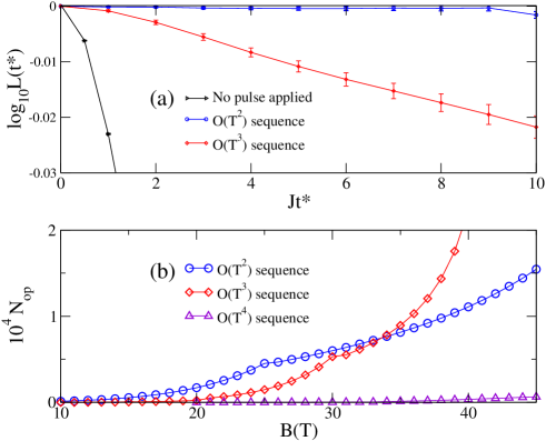
Figure 7: (Color online) (a) Effective dynamics of $L(t^{*})$ for lower orders optimized sequences shows better coherence than that of the original dynamics. Here $J\delta t=0.01$, $\epsilon=-0.3$, and $t^{*}=t/T_{c}(B)$ with $B=20T$. (b)$N_{op}$ for different orders versus $B$ fields. In low fields, $O(T^{2})$ sequence is the optimized. For modest high fields, $O(T^{3})$ sequence starts to win over $O(T^{2})$ sequence.

IV Short Time and long time Dynamics of Two Qubits

In this section, we extend the construction of pulse sequence to multi-qubits. In particular, we shall examine the validity of our construction for two qubits using t-DMRG. We start by considering $n$ qubits denoted by $\vec{\sigma}^{i}$ with $i=1,2,\cdots,n$. Following the derivation of Eqs.(21) and (24), one can move all the spin operators due to the decoupling pulses to the left and obtain the corresponding $G^{N}(t)$. The decoupling sequence generally introduces different history of sign characterized by $f^{i}_{\mu}(t)$. We find $G^{N}(t)=\mathcal{T}e^{-i\frac{\epsilon}{2}\int_{0}^{t}ds\hat{R}(s)}$ with $\hat{R}(s)$ is given by

$$\hat{R}(s)=\sum_{i}\left[f^{i}_{x}(s)\sigma^{i}_{x}S^{x}_{i}(s)+f^{i}_{y}(s)\sigma^{i}_{y}S^{y}_{i}(s)+f^{i}_{z}(s)\sigma^{i}_{z}S^{z}_{i}(s)\right].$$ (39)

If one assumes that different sequence is applied to different qubit, it is clear that in addition to constraints set by Eqs.(29), (32), (34) and (35), there will be extra constraints due to cross product of different qubit spins. Therefore, it is clear that minimum number of pulses can be achieved by setting all the pulse sequence the same: $f^{i}_{\mu}(t)\equiv f_{\mu}(t)$. In this case, we find

$$\hat{R}(s)=f_{x}(s)Q_{x}(s)+f_{y}(s)Q_{y}(s)+f_{z}(s)Q_{z}(s),$$ (40)

where $Q_{\mu}(s)=\sum_{i}\sigma^{i}_{\mu}S^{\mu}_{i}(s)$. In comparison to the case of a single qubit, here $Q_{\mu}$ replaces the role of $\sigma_{\mu}S_{\mu}$. The commutators of $Q_{\mu}$ are given

$$[Q_{\mu}(s),Q_{\nu}(s^{\prime})]=\sum_{i,j}\sigma^{i}_{\mu}\sigma^{j}_{\nu}[S^{\mu}_{i}(s),S^{\nu}_{j}(s^{\prime})].$$ (41)

According to Eq.(25), the $O(s^{n})$ of $S^{\mu}_{i}(s)$ is a n-fold commutator of $H_{bath}$ and $S^{\mu}_{i}$. Since $H_{bath}$ only contains couplings between nearest neighboring $S^{\mu}_{i}$, to $O(s^{n})$, $S^{\mu}_{i}(s)$ contains spin operators up to $S^{\alpha}_{i\pm n}$. Therefore, to $O(s^{n}{s^{\prime}}^{m})$ (i.e., to $O(T^{n+m+1})$), we find $[S^{\mu}_{i}(s),S^{\nu}_{j}(s^{\prime})]=0$ if $|i-j|>n+m$. Consequently, commutators of $Q_{\mu}$ become

$$[Q_{\mu}(s),Q_{\nu}(s^{\prime})]=\sum_{i}\sigma^{i}_{\mu}\sigma^{i}_{\nu}[S^{\mu}_{i}(s),S^{\nu}_{i}(s^{\prime})].$$ (42)

It is then clear that for spin-$1/2$ qubits, because $\sigma^{2}_{\mu}=1$, only commutators with $\mu\neq\nu$ contribute dynamics. Furthermore, coefficients that are associated with these commutators are exactly the same as those for a single qubit. Hence Eqs.(29), (32), (34), and (35) are also the constraints for two qubits to suppress $U(T)$ to $O(T^{4})$. In other words, both the entanglement of two qubit and decoherence of a single qubit can be optimized by the same sequence.

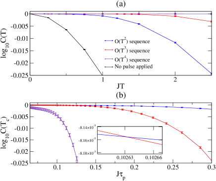
Figure 8: (Color online) (a) Concurrence $C(T)$ versus $T$ of different orders simulated by t-DMRG for Heisenberg-like coupling with $\epsilon=-0.3$. Clearly, $C(T)$ gets improved for increasing number of orders. (b) $C(T_{c})$ versus $J\tau_{p}$. It is clear that as $\tau_{p}$ decreases, $O(T^{3})$ sequence starts to win over $O(T^{2})$ sequence.

To check the validity of the above conclusion, we examine the entanglement of two qubits. To characterize the entanglement, we shall use concurrence as the measurement of entanglement.Wootters For a given reduced density matrix $\rho(t)$, the concurrence is defined as $C=\max\{\lambda_{1}-\lambda_{2}-\lambda_{3}-\lambda_{4},0\}$, where $\lambda_{1}\geq\lambda_{2}\geq\lambda_{3}\geq\lambda_{4}$ are the square roots of the eigenvalues of the operator $\rho(\sigma^{y}\otimes\sigma^{y})\rho^{*}(\sigma^{y}\otimes\sigma^{y})$ and $\rho^{*}$ is the complex conjugation of $\rho$. In Fig. 8(a), we show the concurrence $C(T)$ calculated by t-DMRG for various sequences. It is seen that the sequence in Eq.(36) indeed outperforms other sequence. In Fig. 8(b) we show numerical results of $C(T_{c})$ versus $J\tau_{p}$ for different orders. It is clearly seen that as $\tau_{p}$ decreases, $O(T^{3})$ sequence starts to win over $O(T^{2})$ sequence. In Fig. 9(a), we show the effective dynamics for the concurrence at $t^{*}=nT$. In comparison to the case without decoupling pulses applied, it is clear that decoupling pulses do improve the entanglement of two qubits. Fig. 9(b) shows that except for $O(T^{4})$ sequence with qubits at (39,40), decoupling pulses also suppress the generation of entanglement. One of the reasons behind the non-suppression of the entanglement generation for the $O(T^{4})$ sequence is due to the large $T_{c}$ required by finite $\tau_{p}$. However, as indicated by Eq.(42), the distance between qubits is also an important factor. As a comparison, $C(t^{*})$ of the $O(T^{4})$ sequence for two-qubits located at different distances, (39,40) versus (30,50), are calculated. It is seen that entanglement generation is suppressed only for qubits located at (30,50), in agreement with conclusions based on Eq.(42). In Fig. 9(c),we plot $N_{op}$ for different orders versus $B$ fields. We find that at modest magnetic field, the lowest order,$m=1$, is the most optimized sequence for preserving the entanglement.

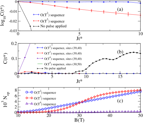
Figure 9: (Color online) (a)Effective dynamics of the concurrency. Here $J\delta t=0.01$, $\epsilon=-0.3$, and $t^{*}=t/T_{c}(B)$ with $B=20T$. (b)Effective dynamics for the generation of entanglement. Here $J\delta t=0.02$, $\epsilon=-0.9$, and $t^{*}=t/T_{c}(B)$ with $B=12T,20T,30T$ for $O(T^{2}),O(T^{3})$, and $O(T^{4})$ sequences respectively. Note that errors are smaller than sizes of figure legends. It is clear that entanglement generation is suppressed for qubits that are far apart. (c)$N_{op}$ obtained from $C(t^{*})$ for different orders versus $B$ fields. In low fields, $O(T^{2})$ sequence is the optimized. For modest high fields, $O(T^{3})$ sequence starts to win over $O(T^{2})$ sequence.

V Summary and Outlook

In summary, feasibility of decoupling pulses that preserve the coherence and entanglement of spin qubits with general couplings to a quantum spin chain are examined. It is shown that error induced by pulse-width accumulation restricts the consideration to sequences with number of pulses being less than $10$ within each cycle. Within each cycle $T$, exact nontrivial pulse sequences are constructed to suppress the qubit-bath coupling to $O(T^{N+1})$ progressively with number of pulses being $4,7,12$ for $N=1,2,3$. It is demonstrated that computing after decoupling has the best performance. Therefore, the performance is examined by counting number of computing pulses that could be applied periodically at the end of each DD cycle. Based on t-DMRG, our numerical results show that for modest magnetic fields (10-40 Tesla) available in laboratories, the overall performance is optimized when number of pulses in each cycle is 4 or 7 with pulse directions be alternating between x and z.

While so far our numerical results are obtained by using either a single qubit or two qubits as demonstrations, our results also provide insights for preserving coherence and entanglement of multi-qubits. In fact, according to our analysis, in principle the same sequences we obtained in this work can also dynamically decouple multi-qubits from the environment in low magnetic fields. For high magnetic fields, to obtain better coherence and entanglement, one needs to suppress higher order terms. In this case, however, one still needs to suppress lower orders. Therefore, our results will still serve as a useful starting point for sequences for higher magnetic fields.

Appendix A $O(T^{3})$ Optimal Sequences

In this appendix, we explicitly construct all possible sequences that suppress $U(T)$ to $O(T^{3})$. For this purpose, we first note that operators appear in $U(T)$ in the order of $O(T)$ and $O(T^{2})$ are $\sigma_{x}S^{x}$, $\sigma_{y}S^{y}$, $\sigma_{z}S^{z}$, $[H_{0},[H_{0},S^{x}]]\sigma_{x}$, $[H_{0},[H_{0},S^{y}]]\sigma_{y}$, and $[H_{0},[H_{0},S^{z}]]\sigma_{z}$. Requiring coefficients of these operators to vanish yields Eqs.(29) and (32). Eqs.(29) and (32) can be solved by using Mathematica to exhaust all possible configurations of pulse directions. We find that in addition to Eq.(33), the following generic sequences are also solutions
Sequence 1: pulse direction $xzxxzx$
$\alpha_{1}=\alpha_{2}=\alpha_{3}=\alpha_{5}=\alpha_{6}=\alpha_{7}=1/8,\alpha_{4}=1/4$
Sequence 2: pulse direction $xzxxyx$
$\alpha_{1}=0.104715$, $\alpha_{2}=0.145282$, $\alpha_{3}=1/8$, $\alpha_{4}=1/4$
$\alpha_{5}=1/8$, $\alpha_{6}=0.145282$, $\alpha_{7}=0.104715$
Sequence 3: pulse direction $xzxzyz$
$\alpha_{1}=0.0785$, $\alpha_{2}=0.1396$, $\alpha_{3}=0.1596$, $\alpha_{4}=1/4$
$\alpha_{5}=0.1715$, $\alpha_{6}=0.0931$, $\alpha_{7}=0.1104$
Sequence 4: pulse direction $xzxyzy$
$\alpha_{1}=1/8$, $\alpha_{2}=0.095491$, $\alpha_{3}=0.1545$, $\alpha_{4}=1/4$
$\alpha_{5}=0.1545$, $\alpha_{6}=0.095491$, $\alpha_{7}=1/8$.
In addition to the above sequences, equivalent sequences can be formed by applying cycle permutations on $x$, $y$ and $z$.

References

- (1) L. Viola and S. Lloyd, Phys. Rev. A 58, 2733 (1998).
- (2) L. Viola, E. Knill, and S. Lloyd, Phys. Rev. Lett. 82, 2417 (1999).
- (3) L. Viola and E. Knill, ibid. 90, 037901 (2003).
- (4) K. Khodjasteh and D. A. Lidar, Phys. Rev. Lett. 95, 180501 (2005).
- (5) K. Khodjasteh and D. A. Lidar, Phys. Rev. A 75, 062310 (2007)
- (6) W. M. Witzel and S. Das Sarma, Phys. Rev. B 76, 241303 (2007).
- (7) G. S. Uhrig, Phys. Rev. Lett. 98, 100504 (2007).
- (8) P. W. Shor, Phys. Rev. A 52, R2493 (1995).
- (9) A. M. Steane, Phys. Rev. Lett. 77, 793 (1996).
- (10) E. Knill and R. Laflamme, Phys. Rev. A 55, 900 (1997).
- (11) P. Zanardi and M. Rasetti, Phys. Rev. Lett. 79, 3306 (1997).
- (12) D. A. Lidar, I. L. Chuang, and K. B. Whaley, Phys. Rev.Lett. 81, 2594 (1998).
- (13) P. Facchi and S. Pascazio, Phys. Rev. Lett. 89, 080401 (2002).
- (14) P. Facchi, D. A. Lidar, and S. Pascazio, Phys. Rev. A 69, 032314 (2004).
- (15) J. R. West, D. A. Lidar, B. H. Fong, M. F. Gyure, X. Peng and D. Suter, arXiv:0911.2398.
- (16) E .L. Hahn, Phys. Rev. 80, 580 (1950).
- (17) U. Haeberlen, High Resolution NMR in Solids (Advances in Magnetic Resonance Series) (Academic, New York,1976).
- (18) Wen Yang and Ren-Bao Liu, Phys. Rev. Lett. 101, 180403 (2008).
- (19) J. R. West, B. H. Fong, and D. A. Lidar, Phys. Rev. Lett. 104, 130501 (2010).
- (20) L. Viola, S. Lloyd, and E. Knill, Phys. Rev. Lett. 83, 4888 (1999).
- (21) Ahmad Abliz, H. J. Gao, X. C. Xie, Y. S. Wu, and W. M. Liu, Phys. Rev. A 74, 052105 (2006).
- (22) D. D. Bhaktavatsala Rao, Phys. Rev. A 76, 042312 (2007).
- (23) Chikako Uchiyama, Masaki Aihara, arXiv:quant-ph/0408139.
- (24) C. J. Shan, W. W. Cheng, T. K. Liu, Y. X. Huang, H. Li, arXiv:0808.3678.
- (25) S. Sachdev, Quantum Phase Transitions, (Cambridge University Press, New York, 1999).
- (26) D. Rossini, T. Calarco, V. Giovannetti, S. Montangero, and R. Fazio, Phys. Rev. A 75, 032333 (2007).
- (27) Cheng-Yan Lai, Jo-Tzu Hung, Chung-Yu Mou, Pochung Chen, Phys. Rev. B 77, 205419 (2008).
- (28) Jo-Tzu Hung, Chung-Yu Mou, Pochung Chen, J. Phys.: Conf. Series, 150, 042131 (2009).
- (29) D. Rossini, P. Facchi, R. Fazio, G. Florio, D. A. Lidar, S. Pascazio, F. Plastina, and P. Zanardi, Phys. Rev. A 77, 052112 (2008).
- (30) W. Magnus, Comm. Pure and Appl. Math. VII:649 V673, (1954).
- (31) Pochung Chen, Phys. Rev. A 73, 022343 (2006).
- (32) William K. Wootters, Phys. Rev. Lett. 80, 2245 (1998).