Driving denaturation: Nanoscale thermal transport as a probe of DNA melting

Abstract

DNA denaturation has been a subject of intense study due to its relationship to DNA transcription and its fundamental importance as a nonlinear structural transition. Many aspects of this phenomenon, however, remain poorly understood. Existing models fit quite well with experimental results on the fraction of unbound base pairs versus temperature, but yield incorrect results for other essential quantities, such as the base pair fluctuation timescales. Here, we demonstrate that nanoscale thermal transport can serve as a sensitive probe of the underlying microscopic physics responsible for the dynamics of DNA denaturation. Specifically, we show that the heat transport properties of DNA are altered significantly as it denatures, and this alteration encodes detailed information on the dynamics of thermal fluctuations and their interaction along the strand. This finding allows for the discrimination between models of DNA denaturation and will help shed new light on the nonlinear vibrational dynamics of this important molecule.

Besides being the “molecule of life” – or perhaps because of it – DNA lives at a unique position where its double-stranded structure can unravel into two single strands, i.e., it denaturates or “melts”, via changes in conditions such as temperature or ionic concentration Sinden (1994). Local melting of DNA due to thermal fluctuations, which can occur well below the denaturation temperature, is thought to play a major role in the formation of the transcription bubble Chen et al. (2010). The denaturation of DNA proceeds via the thermal breakage (dissociation) of base pairs and a nonlinear interaction between base pairs sharpens this transition via cooperative effects in base pair unbinding Peyrard and Bishop (1989); Dauxois et al. (1993a, b). As a result, the accurate description of mechanisms of DNA denaturation requires one to not only correctly account for local thermal fluctuations but also how these fluctuations interact along the strand. These processes are typically probed indirectly through the measurement of the DNA melting curve – the fraction of unbound base pairs versus temperature at equilibrium – thus hindering the understanding of the denaturation mechanisms. However, thermal fluctuations and their interaction along the strand are the same processes that occur in thermal transport, which, as we shall see, can give an independent and more direct assessment of the proposed DNA denaturation mechanisms.

During the past decade, there has been tremendous progress in measuring the thermal and electronic properties of molecular systems Dubi and Di Ventra (2011); Heath (2009), including a recent experiment on the heat conduction of inhomogeneous DNA-Gold nanocomposites Kodama et al. (2009). However, except for few studies relevant to double-stranded DNA Terraneo et al. (2002); Peyrard (2006); Savin et al. (2010), no existing analysis of thermal transport takes into account DNA’s large structural fluctuations that eventually result in its denaturation.

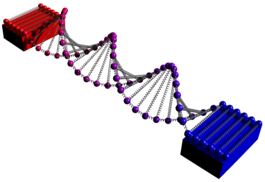
Figure 1: Schematic of DNA between two heat reservoirs that probe its structure via an energy current.

In this paper, the non-equilibrium behavior of single-coordinate nonlinear models of DNA are analyzed as heat is driven through DNA via two thermal reservoirs, as shown schematically in Fig. 1. The preeminent single-coordinate model for thermally driven denaturation of DNA is the Peyrard-Bishop-Dauxois (PBD) model Peyrard and Bishop (1989); Dauxois et al. (1993a, b), which is believed to capture the main physical processes behind DNA denaturation Peyrard (2004). By first deriving an analytic expression for the thermal conductance, $\kappa$, we show that the PBD model predicts a substantial jump in $\kappa$ upon DNA denaturation. That is, the conductance of DNA is predicted to actually increase, despite the fact that the DNA becomes disordered as it is broken into two single strands. This change is a delicate balance of the model parameters and the mechanisms that it represents. Indeed, we show that another related model Joyeux and Buyukdagli (2005), which also can describe the statistical properties of DNA denaturation, gives qualitatively different non-equilibrium behavior, predicting a drop in $\kappa$. Thus, by driving DNA out of equilibrium, the basic physical aspects of denaturation – thermal fluctuations and their coupling along the molecule – can be probed.

We begin with a description of the PBD model Dauxois et al. (1993a). This model, as well as other single-coordinate models for DNA, reduces the DNA strand to a one-dimensional, classical lattice with each base pair represented by a single coordinate – the collective stretching of the hydrogen bonds in a Watson-Crick pair. The PBD Hamiltonian takes on the form

$$H=\sum_{n}\left[\frac{m\dot{y}_{n}^{2}}{2}+V\left(y_{n}\right)+W\left(y_{n},y_{n-1}\right)\right],$$ (1)

where $y_{n}$ represents the stretching coordinate within the $n^{{\rm th}}$ base pair. An on-site Morse potential, $V(y_{n})=D(e^{-ay_{n}}-1)^{2}$, describes the harmonic binding of the base pair at small $y_{n}$ with the angular frequency $\sqrt{2Da^{2}/m}$, and unbinding at $y_{n}\gg a$ with the finite dissociation energy $D$. The PBD nearest-neighbor potential is given by

$$W(y_{n},y_{n-1})=\frac{K}{2}(1+\rho e^{-\alpha(y_{n}+y_{n-1})})(y_{n}-y_{n-1})^{2}.$$ (2)

The PBD model has been quite successful in characterizing statistical properties of DNA near the denaturation transition Campa and Giansanti (1998); Weber et al. (2009). However, since it was not derived from a microscopic Hamiltonian, one has to validate the model by comparison with experimental results. In this regard, there is a considerable ambiguity in the results for short DNA strands Campa and Giansanti (1998); Peyrard et al. (2008); Sanrey and Joyeux (2009); Ares et al. (2009) as well as the timescales for the opening of bubbles at room temperature Peyrard et al. (2008, 2009). Thermal transport, as we show below, can determine some of the main features single-coordinate models should display (beyond equilibrium denaturation curves) and help settle the above discrepancies.

We start our analysis by examining the behavior of the PBD model in the low ($L$) and high ($H$) temperature limits, where it becomes harmonic with the effective Hamiltonian

$$H_{\mu}=\sum_{n}\left[\frac{m\dot{y}_{n}^{2}}{2}+D_{\mu}y_{n}^{2}+\frac{K_{\mu}}{2}\left(y_{n}-y_{n-1}\right)^{2}\right],$$ (3)

with $\mu=L,\,H$. Numerical studies show that the full PBD model, described by the Hamiltonian in Eq. (1), undergoes a sharp transition corresponding to the denaturation of DNA Dauxois et al. (1993b). Above the transition temperature, $T_{c}$, the base pairs become unbound, i.e., the on-site potential approaches a constant leading to $D_{H}=0$. The nearest-neighbor potential becomes harmonic with $K_{H}=K$. In the low temperature limit, the strand will again have harmonic behavior with the parameters of the effective Hamiltonian $D_{L}=Da^{2}$ and $K_{L}=K\left(1+\rho\right)$ (the latter reflects the larger nearest-neighbor coupling of the low temperature strand). Even at low-temperatures, the nonlinearity of the potential is important, but the harmonic limit gives the correct physical interpretation of the numerical results on the full model we present later.

We introduce the concept of the thermal conductance ratio, $R$, as the ratio of the conductance between the high and low temperature phases $R\equiv\kappa_{H}/\kappa_{L}$. For Ohmic heat reservoirs strongly coupled to the first and last site of the strand, it can be calculated to be (see Appendix A and Refs. Casher and Lebowitz (1971); Dhar (2001) for details)

$$R\approx\frac{2K_{H}D_{L}}{K_{L}^{2}},$$ (4)

which uses the lowest order term in $K_{L}/D_{L}$ for $\kappa_{L}$ (see Eq. (16) in Appendix A). Since Eq. (4) is for strong coupling, it represents an extreme value for $R$. For the PBD model with the original parameters from Ref. Dauxois et al. (1993a), the corresponding ratio is $R_{PBD}\approx 18$ ftn (a). That is, the transition from low to high $T$ results in a substantial jump in $\kappa$ due to the weakening of the on-site confining potential, i.e., the base pair dissociation, as $T$ crosses $T_{c}$ from below. The removal of the on-site potential softens the modes of the strand, making them more efficient in the transport of heat. This is more transparent if one examines the low temperature conductance,

$$\kappa_{L}\propto\frac{K_{L}^{2}}{D_{L}}\propto\frac{K_{L}^{2}}{m\omega_{L}^{2}},$$ (5)

where $\omega_{L}$ is the on-site frequency and we have taken $K_{L}/D_{L}$ to be small. Equation (5) shows that the conductance increases with decreasing frequency.

We note that the PBD model give a novel phenomenon compared to other transitions. For example, in the ice-water transition at 273 K, the conductance decreases, rather than increases, with a ratio of $R_{\mathrm{H_{2}O}}\approx 0.25$ Lide (2009). This is mainly due to the breaking of crystal structure across the transition that reduces the coupling between molecules. Another example is single-crystal C₆₀, which exhibits a face-centered-cubic to simple-cubic structural transition at 260 K Yu et al. (1992). The ratio for this transition can be estimated from the experimental data to be $R_{C_{60}}\approx 0.75$.

The thermal conductance ratio is thus important in identifying the underlying mechanisms of a structural transition. The balance of the softening of the lattice and the reduction of the nearest neighbor coupling determines both the magnitude of the conductance change, as well as whether it increases or decreases. Different proposals for the nonlinear forms of the model will give different limiting harmonic forms, changing the conductance behavior across the temperature range not only quantitatively, but also qualitatively. For example, another single-coordinate model of DNA is that of Joyeux and Buyukdagli (JB) in Ref. Joyeux and Buyukdagli (2005). It uses the same on-site potential but employs an alternative nearest-neighbor potential that, although giving a very similar melting curve, results in a different high temperature harmonic Hamiltonian (see Appendix A). In the strong-coupling limit, $R$ changes as

$$R_{PBD}\approx 18\longrightarrow R_{JB}\approx 0.017.$$

That is, the PBD model gives qualitatively distinct behavior from the JB model because the latter looses virtually all of its nearest neighbor coupling at high temperature, i.e., it looks more like the ice-to-water transition in character. This qualitative conclusion does not change even when using different parameter sets that have been developed ftn (b). Therefore, while they both agree well with some denaturation experiments, the conductance ratio can be used to directly probe the physics contained within their respective interaction potentials. While temperatures much higher than the transition temperature are beyond the validity of the models, the opposing predictions persist within a range of temperatures, including around the denaturation transition. In addition, having the ends of the DNA “clamped” together on each of the heat reservoirs – one way to measure its thermal transport properties – will help the fluctuations described by these single-coordinate models to persist to higher temperatures. This strongly supports using the heat conduction as a test to determine basic aspects of DNA denaturation that need to be represented in microscopic models.

To gain further insight into the non-equilibrium behavior of DNA, we solve for the full dynamics of the PBD model (Eq. (1) with the appropriate stacking interaction) by numerically integrating the equations of motion of the DNA between two Langevin reservoirs (see Appendix B for details on numerical simulations). In Fig. 2(a), we plot the thermal current as a function of the average reservoir temperature, while keeping the temperature difference constant at a value significantly lower than the width of the phase transition so that the entire strand is always in one phase.

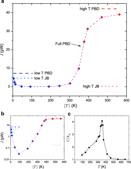
Figure 2: Thermal transport across the denaturation transition. (a) Thermal current through DNA as a function of average temperature, $\langle T\rangle=\left(T_{L}+T_{H}\right)/2$, calculated while keeping the temperature difference $\Delta T=T_{H}-T_{L}=9.3\,\mathrm{K}$ constant. The thermal current displays a steep rise as the temperature crosses the transition temperature $T_{c}\simeq 350\,\mathrm{K}$. Low and high temperature simulations of the harmonic strands defined by $H_{L}$ and $H_{H}$ are given by blue and red lines, respectively. The numerical results on the full PBD model approach the harmonic limits at sufficiently low and high temperatures. (b) Logarithmic scale plot of the thermal current. The convergence to the harmonic limit, as well as an non-monotonic dependence of the thermal current on temperature at low temperatures and a sharp rise near the transition are visible. The latter indicates that DNA may be suitable to function as a molecular thermal switch. (c) Dependence of equilibrium heat capacity, $C$, (normalized per length of the strand) on temperature showing the transition at $T_{c}$ and the convergence to the harmonic value $C/k_{B}=1$. The convergence to the harmonic value at high temperature is much more rapid than a low temperature, indicating that the anharmonicity of the Morse potential is still important even at low temperature.

As seen Fig. 2, the ability of the DNA to conduct heat increases substantially after it becomes denaturated according to the PBD model, thus confirming our analytical prediction. Further, the conductivity at $\langle T\rangle=300\,\mathrm{K}$ is 0.18 pW/KÅ – smaller than that in Ref. Savin et al. (2010). The difference is due to different interactions taken into account, which result in an absence of any signatures of denaturation up to 350 K in Ref. Savin et al. (2010). Thus, their results do not incorporate the effect of strong nonlinearities due to denaturation/local melting. We have also calculated the thermal current for purely harmonic strands with the parameters corresponding to the different phases (as discussed below Eq. (3)). The thermal conductance ratio for the harmonic limits is found numerically to be $R_{PBD}\approx 6$, which is lower than our analytical result due to the more realistic reservoir implemented in our simulations (see Appendix B). Figure 2(c) plots the heat capacity $C$ (per base pair) as a function of temperature, indicating the denaturation transition and the approach to harmonicity (where $C/k_{B}$ is always unity).

The nonlinear model, however, gives much richer behavior. While at high temperature there is convergence of the nonlinear model to its harmonic limit, at low temperatures a non-monoticity appears, more clearly seen in Fig. 2(b) where we plot the thermal current as a function of temperature on a logarithmic scale. The non-monotonicity, reflected in the drop of $\kappa$ in the temperature range $0-100$ K, is mainly due to phonon scattering off the anharmonic on-site potential. This signature – conductance versus temperature – indicates the strength of the nonlinearity in DNA dynamics, which we will investigate further in a future contribution. Although the single-coordinate models we study here were proposed to study DNA behavior near the denaturation transition, such a nonlinear signature should still appear at low temperature, implying that a measurement of DNA thermal transport could also serve to define the temperature range of validity of the PBD model. It also gives rise to a three orders of magnitude increase of the thermal conductance, indicating that this characteristic of structural phase transitions can be useful in developing heattronic devices such as thermal switches and thermal transistors Chien et al. (2011).

In the above discussion we have considered only homogeneous DNA strands. It is clear that heterogeneity will give rise to interesting effects in the conductance. Alternating sequences of AT and GC pairs, for instance, will tend to suppress the low temperature conductance due to the mismatch between parameters of base pair binding potentials, while the high temperature conductance will remain roughly the same. This will result in a substantial increase in $R$ Chien et al. (2011), which will also occur due to random or genomic DNA. Differences between AT and GC pairs gives an additional experimental test of this class of models Chien et al. (2011).

To conclude, we have investigated the out-of-equilibrium properties of single-coordinate models of DNA in order to elucidate the nonlinear nature of denaturation. The balance of lattice softening and reduced coupling in different models leads to qualitatively distinct predictions for the thermal conductance ratio – the experimental measurement of which will illuminate these fundamental aspects of DNA and thus should shed light on the underlying mechanisms of DNA denaturation. Due to the nature of the effect, experiments will be robust with respect to heterogeneity, defects, and contacts, unlike the electrical counterpart Di Ventra and Zwolak (2004). Recent experiments on the heat conduction of nanotubes Kim et al. (2001) and DNA-Gold nanocomposites Kodama et al. (2009) give a potential route to developing the experimental setup. However, it will be necessary to perform the experiment in conditions of high humidity so the DNA retains its B-form Record et al. (1981). Such an experiment could also be done on double- and single- stranded DNA separately, which would remove uncertainties due to the lack of solvent. Fluorescence experiments to detect local openings of the DNA strand Bonnet et al. (1998); Altan-Bonnet et al. (2003) can further complement the thermal transport measurements. The thermal conductance ratio may also be useful in understanding other structural transitions, such as nanotube collapse. Finally, such experiments will pave the road to creating molecular thermal switches and open new avenues in understanding and controlling thermal flow at the nanoscale.

Appendix A Analytic derivation of the thermal conductance

The thermal conductance of a classical harmonic lattice can be found analytically. Our starting point is the procedure of Refs. Casher and Lebowitz (1971); Dhar (2001). We consider the limiting cases of the single-coordinate Hamiltonian, Eq. (1), for a lattice of length $N$. One already saw that the low- (L) and high- (H) temperature limits can be approximated by a harmonic Hamiltonian of the form

$$H_{\mu}=\sum_{n}\left[\frac{m\dot{y}_{n}^{2}}{2}+D_{\mu}y_{n}^{2}+\frac{K_{\mu}}{2}\left(y_{n}-y_{n-1}\right)^{2}\right],$$ (6)

where $\mu=L,\>H$.

To simplify the analysis, the lattice is coupled to two heat reservoirs at the first and last sites, which gives the equations of motion

$$m\ddot{y}_{n} =-2(D_{\mu}+K_{\mu})y_{n}+K_{\mu}(y_{n-1}+y_{n+1})$$

$$+(\delta_{n,1}+\delta_{n,N})\left[\int_{-\infty}^{t}dt^{\prime}A(t-t^{\prime})y_{n}(t^{\prime})+\eta_{n}(t)\right].$$ (7)

We choose the spectrum of the dissipation to be ohmic, $A(\omega)=-i\gamma\omega$, with coupling $\gamma$, and the noise to be white noise, $\langle\eta_{L/H}(\omega)\eta_{L/H}(\omega^{\prime})\rangle=4\pi T_{L/H}\gamma\delta(\omega+\omega^{\prime})$, with $T_{L/H}$ the low and high reservoir temperatures. This form for the reservoirs will satisfy the fluctuation-dissipation theorem. The resulting equations of motion are

$$m\ddot{y}_{n} =-2(D_{\mu}+K_{\mu})y_{n}+K_{\mu}(y_{n-1}+y_{n+1})$$

$$+(\delta_{n,1}+\delta_{n,N})\left[-\gamma\dot{y}_{n}(t)+\eta_{n}(t)\right].$$ (8)

The solution for the coordinates has the form

$$y_{n}(t)=(1/2\pi)\int_{-\infty}^{\infty}d\omega\hat{Y}_{nm}^{-1}(\omega)\hat{\eta}_{m}(\omega)e^{i\omega t},$$ (9)

where $\hat{\eta}$ is a vector of length $N$ with the first and last components being $\eta_{L/H}(\omega)$ and the rest being zero. It represents the coupling of the reservoirs to the ends of the lattice. The $N\times N$ matrix $\hat{Y}=\hat{\phi}-\omega^{2}\hat{M}-\hat{A}$ encodes the solution. Here $\hat{\phi}_{nm}=2(D_{\mu}+K_{\mu})\delta_{n,m}-K_{\mu}\delta_{n,m+1}-K_{\mu}\delta_{n,m-1}$, $\hat{M}_{ij}=m\delta_{i,j}$, and $\hat{A}_{11}=\hat{A}_{NN}=A(\omega)$ and $\hat{A}_{nm}=0$ otherwise.

The heat current flowing into the lattice is $J=\langle[\int_{-\infty}^{t}dt^{\prime}A(t-t^{\prime})y_{1}(t^{\prime})]\dot{y}_{1}(t)\rangle$, where the average is over the noise. Setting $\gamma=\lambda m$, the heat current becomes

$$J_{\mu} =\frac{\Delta T\lambda^{2}m^{2}}{\pi}\int_{-\infty}^{\infty}d\omega\omega^{2}\{(\mathcal{D}_{1,N}-\lambda^{2}\omega^{2}m^{2}\mathcal{D}_{2,N-1})^{2}$$

$$+\lambda^{2}\omega^{2}m^{2}(\mathcal{D}_{1,N-1}+\mathcal{D}_{2,N})^{2}\}^{-1}|C_{1,N}|^{2},$$ (10)

where $\Delta T=T_{H}-T_{R}$ is the temperature difference of the reservoirs, $C_{1,N}$ is the cofactor of $\hat{Y}_{1,N}$, and $\mathcal{D}_{n,m}$ is the determinant of the submatrix of $(\hat{\phi}-\omega^{2}\hat{M})$ from the $n$-th row (column) to the $m$-th row (column). It follows that $|C_{1,N}|^{2}=K_{\mu}^{2N-2}$ and $\mathcal{D}_{n,m}=K_{\mu}^{n-m+1}\mathcal{D}_{n,m}^{0}$. The elements of $\mathcal{D}_{nm}^{0}$ are given by $\left(\begin{array}[]{cc}\mathcal{D}_{1,N}^{0}&-\mathcal{D}_{1,N-1}^{0}\\ \mathcal{D}_{2,N}^{0}&-\mathcal{D}_{2,N-1}^{0}\end{array}\right)=\mathcal{T}^{N}$, where

$$\mathcal{T}=\left(\begin{array}[]{cc}2(1+D_{\mu}/K_{\mu})-(m/K_{\mu})\omega^{2}&-1\\ 1&0\end{array}\right).$$ (11)

We look for the eigenvalues of $\mathcal{T}$ of the form $\exp(\pm iq)$ with real $q$ because those eigenvalues correspond to propagating modes. This requirement imposes that $2\cos(q)=2(1+D_{\mu}/K_{\mu})-(m/K_{\mu})\omega^{2}$. After changing variables from $\omega$ to $q$ that satisfy this constraint, the final expression (for an infinite lattice ($N\rightarrow\infty$)) is

$$\frac{J_{\mu}}{\Delta T}=\frac{\gamma}{2\pi m}\int_{0}^{2\pi}dq\frac{\sin^{2}(q)}{1+\frac{2\gamma^{2}}{mK_{\mu}}\left[1+\frac{D_{\mu}}{K_{\mu}}-\cos(q)\right]}.$$ (12)

This gives, explicitly for the low and high temperature thermal conductance $\kappa_{\mu}=J_{\mu}/\Delta T$,

$$\kappa_{\mu}=\frac{k_{B}mK_{\mu}^{2}}{4\gamma^{3}}\left[1+\frac{2\gamma^{2}}{mK_{\mu}}+\frac{2\gamma^{2}D_{\mu}}{mK_{\mu}^{2}}-\mathcal{B_{\mu}}\right],$$ (13)

with

$$\mathcal{B}_{\mu}=\sqrt{1+\frac{4\gamma^{2}}{mK_{\mu}}+\frac{4\gamma^{2}D_{\mu}}{mK_{\mu}^{2}}+\frac{8\gamma^{4}D_{\mu}}{m^{2}K_{\mu}^{3}}+\frac{4\gamma^{4}D_{\mu}^{2}}{m^{2}K_{\mu}^{4}}}.$$ (14)

With these expressions one can explicitly find the thermal conductance ratio $R$. We have verified that for reservoirs contacted to a single site on each end, the thermal conductance from our numerical simulations agree with our analytic formula to within $10-15$%, which we attribute to finite size effects in the numerical simulations.

We can take various limiting forms of these equations. If we define the prefactor as $\tilde{\kappa}_{\mu}$ and a dimensionless reservoir coupling as

$$\gamma_{\mu}=\frac{\gamma}{\sqrt{mK_{\mu}}},$$ (15)

the expressions for the conductance become

$$\kappa_{\mu}=\tilde{\kappa}_{\mu}\left[1+2\gamma_{\mu}^{2}+2\gamma_{\mu}^{2}\frac{D_{\mu}}{K_{\mu}}-\mathcal{B_{\mu}}\right],$$ (16)

with

$$\mathcal{B}_{\mu}=\sqrt{1+4\gamma_{\mu}^{2}+4\gamma_{\mu}^{2}\frac{D_{\mu}}{K_{\mu}}+8\gamma_{\mu}^{4}\frac{D_{\mu}}{K_{\mu}}+4\gamma_{\mu}^{4}\left(\frac{D_{\mu}}{K_{\mu}}\right)^{2}}.$$ (17)

The appropriate limiting forms for our case are the following. When the high temperature harmonic limit has no onsite potential, then the heat conductance becomes

$$\kappa_{H}=\tilde{\kappa}_{H}\left[1+2\gamma_{H}^{2}-\sqrt{1+4\gamma_{H}^{2}}\right].$$ (18)

For a low temperature limit that has a much greater onsite term than the nearest neighbor coupling, i.e., $K_{L}/D_{L}\ll 1$, the heat conductance becomes

$$\kappa_{L}\approx\frac{\tilde{\kappa}_{L}\gamma_{L}^{2}K_{L}}{D_{L}},$$ (19)

which also assumes that the dimensionless coupling to the reservoirs is $\gamma_{L}\geq 1$. For strong coupling to the reservoirs, the ratio becomes

$$R\approx\frac{2K_{H}D_{L}}{K_{L}^{2}}.$$ (20)

This is the analytic expression we use within the article. The strong coupling limit gives the extreme value of $R$.

Now we show that the characteristic frequency in the PBD model is lowered as $T$ crosses $T_{c}$ from below. For the low temperature Hamiltonian, the corresponding equation of motion is

$$m\ddot{y}_{n}=-\{2Da^{2}y_{n}+K(1+\rho)[(y_{n}-y_{n-1})+(y_{n}-y_{n+1})]\}.$$ (21)

From the ansatz $y_{n}=y_{n}^{0}e^{i\omega t-ikn}$ , one obtains the phonon spectrum as

$$m\omega^{2}=2Da^{2}+2K(1+\rho)[1-\cos(k)].$$ (22)

Thus, the frequency band of phonons is $\sqrt{2Da^{2}/m}\leq\omega\leq\sqrt{[2Da^{2}+4K(1+\rho)]/m}$. For the high temperature Hamiltonian, the equation of motion is

$$m\ddot{y}_{n}=-K[(y_{n}-y_{n-1})+(y_{n}-y_{n+1})]$$ (23)

and the phonon spectrum is

$$m\omega^{2}=2K[1-\cos(k)].$$ (24)

The frequency band of phonons is $0\leq\omega\leq\sqrt{4K/m}$. The two limiting Hamiltonians are both harmonic and the characteristic frequency is indeed lowered, and similar considerations apply for other models. In the low temperature limit, the onsite potential stiffens the DNA compared to the high temperature limit, which results in the raising of the phonon spectrum of the low temperature limit compared to the high temperature. In the latter, as well, the nearest neighbor coupling drops from $K\left(1+\rho\right)$ to $K$ shrinking the bandwidth. This trade-off is responsible for the change in thermal conductance across the transition. If the drop in nearest neighbor coupling is small, then the softening will dominate, and the heat conductance will increase because these softened modes can conduct heat more effectively.

Appendix B Numerical Simulation Details

To study the dynamics of the DNA out of equilibrium we solve numerically the Langevin equation, which describes the dynamics of a Hamiltonian system in the presence of thermal baths. The Langevin equation is given by

$$m\ddot{y}_{n}=-\frac{\partial W}{\partial y_{n}}-\frac{\partial V}{\partial y_{n}}-\Gamma_{n}\dot{y}_{n}+f(t),$$ (25)

where $W(y_{n})$ and $V(y_{n})$ are the potentials described in Eq. (1). The DNA strand is split into three regions, the two ends, each of length $l$, serve as the Langevin thermal reservoirs at temperatures $T_{L}$ and $T_{H}$. This means that the friction term $\Gamma_{n}$ only operates for $n$ within the thermal reservoirs. The fluctuating term $f(t)$ is Gaussian white noise which obeys the fluctuation-dissipation relation $\langle f(t)f(t^{\prime})\rangle=2\Gamma_{n}k_{B}T_{L(H)}\delta(t-t^{\prime})$ for the low and high temperature reservoirs, respectively.

The middle region of the length $M$ is the free DNA strand, which is driven out of equilibrium by the Langevin reservoirs when $T_{L}\neq T_{H}$. The parameters for the simulations are $M=60$ and $l=20$, and the PBD model parameters are $D=0.04\,\mathrm{eV}$, $a=4.47\,\textrm{\AA}^{-1}$, $K=0.04\,\mathrm{eV/\textrm{\AA}^{2}}$ , $m=300\,\mathrm{u}$, $\rho=0.5$, and $\alpha=0.358\,\textrm{\AA}^{-1}$ Dauxois et al. (1993a). The strand is homogeneous DNA except for the random forces and friction in the Langevin regions. The equations of motion are integrated with the fourth-order Runge-Kutta method. The temperature profile of the strand is evaluated by defining the local temperature at site $n$ as $k_{B}T_{n}^{loc}=m\langle\dot{y}_{n}^{2}\rangle$, where the average is over time. The local heat current is given by $J_{n}=-\left\langle\dot{y}_{n}\frac{\partial W(y_{n},y_{n-1})}{\partial y_{n}}\right\rangle$. The simulations are performed long enough to allow the system to reach its steady state.

The simulations of the heat capacity were performed by connecting Langevin reservoirs of identical temperature to every site in the chain and evaluating the average energy per site by $E=\left\langle\frac{m\dot{y}_{n}^{2}}{2}+V(y_{n})+W(y_{n},y_{n-1})\right\rangle$, where the averaging is performed over time and all the sites of the chain. Then, the dependence of average energy per site on temperature, $E(T)$, obtained by scanning through a set of temperature points, was numerically differentiated to yield the heat capacity.

We also performed simulations on the JB model Joyeux and Buyukdagli (2005), which has the same onsite potential as the PBD model and uses the nearest neighbor potential

$$W(y_{n},y_{n-1})=K_{b}(y_{n}-y_{n-1})^{2}+\frac{\Delta H}{2}(1-e^{-b(y_{n}-y_{n-1})^{2}}).$$ (26)

The parameters in this interaction are $K_{b}=10^{-5}\,\mathrm{eV/\textrm{\AA}^{2}}$, $\Delta H=0.44\,\mathrm{eV}$, and $b=0.1\,\mathrm{\textrm{\AA}}^{-2}$. Thus, the low temperature limit is $K_{L}^{JB}=2K_{b}+b\Delta H$, with $D_{L}^{JB}=D_{L}$. The coupling $K_{L}^{JB}=0.044\,\mathrm{eV/\textrm{\AA}^{2}}$ is not substantially different from the PBD model, which has $K_{L}=0.06\,\mathrm{eV/\textrm{\AA}^{2}}$. However, numerical simulations indicate that in the high temperature limit the heat conductance converges to the conductance of a harmonic Hamiltonian with nearest neighbor interaction $K_{b}(y_{n}-y_{n-1})^{2}$. In other words, the quantity $(y_{n}-y_{n-1})^{2}$ is sufficiently large to suppress the second term in Eq. (26). Thus, the high temperature effective nearest neighbor coupling is $K_{H}^{JB}=2K_{b}$, which is substantially smaller than the low temperature coupling, and also substantially smaller than the high temperature coupling of the PBD model.

References

- Sinden (1994) R. D. Sinden, DNA Structure and Function (Academic Press, London, UK, 1994), 1st ed.
- Chen et al. (2010) J. Chen, S. A. Darst, and D. Thirumalai, Proc. Natl. Acad. Sci. U. S. A. 107, 12523 (2010).
- Peyrard and Bishop (1989) M. Peyrard and A. R. Bishop, Phys. Rev. Lett. 62, 2755 (1989).
- Dauxois et al. (1993a) T. Dauxois, M. Peyrard, and A. R. Bishop, Phys. Rev. E 47, R44 (1993a).
- Dauxois et al. (1993b) T. Dauxois, M. Peyrard, and A. R. Bishop, Phys. Rev. E 47, 684 (1993b).
- Dubi and Di Ventra (2011) Y. Dubi and M. Di Ventra, Rev. Mod. Phys. 83, 131 (2011).
- Heath (2009) J. R. Heath, Annu. Rev. Mater. Res. 39, 1 (2009).
- Kodama et al. (2009) T. Kodama, A. Jain, and K. E. Goodson, Nano Lett. 9, 2005 (2009).
- Terraneo et al. (2002) M. Terraneo, M. Peyrard, and G. Casati, Phys. Rev. Lett. 88, 094302 (2002).
- Peyrard (2006) M. Peyrard, EPL (Europhysics Letters) 76, 49 (2006).
- Savin et al. (2010) A. V. Savin, M. A. Mazo, I. P. Kikot, L. I. Manevitch, and A. V. Onufriev, arXiv:1010.0363 (2010).
- Peyrard (2004) M. Peyrard, Nonlinearity 17, R1 (2004).
- Joyeux and Buyukdagli (2005) M. Joyeux and S. Buyukdagli, Phys. Rev. E 72, 051902 (2005).
- Campa and Giansanti (1998) A. Campa and A. Giansanti, Phys. Rev. E 58, 3585 (1998).
- Weber et al. (2009) G. Weber, J. W. Essex, and C. Neylon, Nat Phys 5, 769 (2009).
- Peyrard et al. (2008) M. Peyrard, S. Cuesta-López, and G. James, Nonlinearity 21, T91 (2008).
- Sanrey and Joyeux (2009) M. Sanrey and M. Joyeux, Phys. Rev. Lett. 102, 029601 (2009).
- Ares et al. (2009) S. Ares, N. K. Voulgarakis, K. Ø. Rasmussen, and A. R. Bishop, Phys. Rev. Lett. 102, 029602 (2009).
- Peyrard et al. (2009) M. Peyrard, S. Cuesta-López, and G. James, Journal of Biological Physics 35, 73 (2009).
- Casher and Lebowitz (1971) A. Casher and J. L. Lebowitz, Journal of Mathematical Physics 12, 1701 (1971).
- Dhar (2001) A. Dhar, Phys. Rev. Lett. 86, 5882 (2001).
- ftn (a) We use the original parameters for the PBD model from Ref. Dauxois et al. (1993a) since there are still discrepancies in what parameters should be used (see, e.g., Refs. Weber et al. (2009); Theodorakopoulos (2010, 2011)). There is a large positive in the PBD model when changing physically relevant parameters, making it a robust feature of the model. Thermal transport measurements, as well, will help settle what parameters actually describe DNA.
- Lide (2009) D. R. Lide, CRC Handbook of Chemistry and Physics (CRC Press (Taylor and Francis Group), Boca Raton, FL, 2009), 90th ed.
- Yu et al. (1992) R. C. Yu, N. Tea, M. B. Salamon, D. Lorents, and R. Malhotra, Phys. Rev. Lett. 68, 2050 (1992).
- ftn (b) For instance, for the parameter sets in Refs. Campa and Giansanti (1998) and Alexandrov et al. (2009), and for those in Refs. Theodorakopoulos (2010, 2011).
- Chien et al. (2011) C.-C. Chien, K. A. Velizhanin, Y. Dubi, and M. Zwolak, in preparation (2011).
- Di Ventra and Zwolak (2004) M. Di Ventra and M. Zwolak, in Encyclopedia of Nanoscience and Nanotechnology, edited by H. Singh-Nalwa (American Scientific Publishers, 2004), vol. 2, p. 475.
- Kim et al. (2001) P. Kim, L. Shi, A. Majumdar, and P. L. McEuen, Phys. Rev. Lett. 87, 215502 (2001).
- Record et al. (1981) M. T. Record, S. J. Mazur, P. Melancon, J. H. Roe, S. L. Shaner, and L. Unger, Annu. Rev. Biochem. 50, 997 (1981).
- Bonnet et al. (1998) G. Bonnet, O. Krichevsky, and A. Libchaber, Proc. Natl. Acad. Sci. U. S. A. 95, 8602 (1998).
- Altan-Bonnet et al. (2003) G. Altan-Bonnet, A. Libchaber, and O. Krichevsky, Phys. Rev. Lett. 90, 138101 (2003).
- Theodorakopoulos (2010) N. Theodorakopoulos, Phys. Rev. E 82, 021905 (2010).
- Theodorakopoulos (2011) N. Theodorakopoulos, arXiv:1102.0259 (to appear J. Nonlinear Math. Phys.) (2011).
- Alexandrov et al. (2009) B. S. Alexandrov, V. Gelev, Y. Monisova, L. B. Alexandrov, A. R. Bishop, K. Ø. Rasmussen, and A. Usheva, Nucleic Acids Res. 37, 2405 (2009).