Abstract

The Alcubierre spacetime was simulated by means of a Tamm medium which is asymptotically identical to vacuum and has constitutive parameters which are continuous functions of the spatial coordinates. Accordingly, the Tamm medium is amenable to physical realization as a nanostructured metamaterial. A comprehensive characterization of ray trajectories in the Tamm medium was undertaken, within the geometric-optics regime. Propagation directions corresponding to evanescent waves were identified: these occur in the region of the Tamm medium which corresponds to the warp bubble of the Alcubierre spacetime, especially for directions perpendicular to the velocity of the warp bubble at high speeds of that bubble. Ray trajectories are acutely sensitive to the magnitude and direction of the warp bubble’s velocity, but rather less sensitive to the thickness of the transition zone between the warp bubble and its background. In particular, for rays which travel in the same direction as the warp bubble, the latter acts as a focusing lens, most notably at high speeds.

PACS numbers: 04.40.Nr, 41.20.-q, 42.15.-i

Keywords: Alcubierre warp drive, Tamm medium, metamaterial, ray tracing

1 Introduction

Metamaterials provide opportunities to study general-relativistic scenarios which would otherwise be either impractical or impossible to explore [1]. This may be achieved by exploiting the formal analogy that exists between light propagation in vacuum subjected to a gravitational field and light propagation in a certain nonhomogeneous bianisotropic medium, known as a Tamm medium [2, 3, 4]. The practical creation of Tamm mediums is beginning to look like an increasingly realistic proposition, as rapid developments are made in the science of nanostructured metamaterials. In recent years, metamaterial-based simulations of black holes [5], cosmic strings [6], de Sitter spacetime [7, 8] and wormholes [9] have been proposed, for example.

As a useful Gedankenexperiment, the spacetime of the Alcubierre metric has generated considerable interest since its introduction in 1994 [10, 11, 12]. The spacetime is characterized by a warp bubble which moves with respect to an asymptotically flat background at a speed $v^{\prime}_{s}c_{\scriptscriptstyle 0}$, where $c_{\scriptscriptstyle 0}$ is the speed of light in the absence of a gravitational field and $v^{\prime}_{s}\geq 0$. By effectively contracting the spacetime ahead of the warp bubble and expanding the spacetime behind it, arbitrary relative speeds $v^{\prime}_{s}$ may be achieved, in principle. In contrast, within the local environment of the warp bubble, its speed is necessarily subluminal; i.e., $v^{\prime}_{s}<1$.

Serious obstacles stand in the way of a physical realization of the Alucbierre spacetime, stemming from violations of various energy constraints [13, 14]. Even the subluminal regime is associated with negative energy densities [15]. However, negative energy densities are not unprecedented in astrophysics. For examples, the emission of Hawking radiation by a black hole is accompanied by a flow of negative energy [16], and the construction of wormholes relies on negative energy density [17]. Nor is negative energy density unprecedented within the realm of metamaterials: propagation of (monochromatic) plane waves with negative phase velocity [18] — which is intimately related to the phenomenon of negative refraction [19] that certain metamaterials have been shown to support in experimental observations [20] — also involves negative energy density [21], at least in the absence of dissipation [22].

In this communication, we present a simulation of the Alcubierre spacetime, in the form a Tamm medium which is physically realizable, in principle. Under the geometric-optics approximation, a comprehensive characterization of light ray trajectories through the Tamm medium is provided.

As regards notation, $3$–vectors are underlined and unit $3$-vectors are additionally distinguished by a caret, whereas 3$\times$3 dyadics [23] are double underlined. The identity dyadic is written as $\underline{\underline{I}}$. The scalar constants $\epsilon_{\scriptscriptstyle 0}$ and $\mu_{\scriptscriptstyle 0}$ denote the permittivity and permeability of vacuum in the absence of a gravitational field, and $c_{\scriptscriptstyle 0}=1/\sqrt{\epsilon_{\scriptscriptstyle 0}\mu_{\scriptscriptstyle 0}}$.

2 Tamm medium for Alcubierre spacetime

The Alcubierre spacetime is specified by the line element [10]

$$ds^{2}=-c_{\scriptscriptstyle 0}^{2}dt^{\prime 2}+\left[dx^{\prime}-v^{\prime}_{s}f(r^{\prime}_{s})c_{\scriptscriptstyle 0}dt^{\prime}\right]^{2}+dy^{\prime 2}+dz^{\prime 2},$$ (1)

for the case where the warp bubble travels at relative velocity $\underline{v}^{\prime}_{s}=v^{\prime}_{s}\,\hat{\underline{x}}^{\prime}$. Herein the scalar function

$$f(r^{\prime}_{s})=\frac{\tanh\left[\sigma\left(r^{\prime}_{s}+R\right)\right]-\tanh\left[\sigma\left(r^{\prime}_{s}-R\right)\right]}{2\tanh\left(\sigma R\right)}$$ (2)

is unit–valued at the origin and decays uniformly to zero as $r^{\prime}_{s}\to\infty$, where $x^{\prime}_{s}(t^{\prime})=v^{\prime}_{s}c_{\scriptscriptstyle 0}t^{\prime}$ and the time-dependent translated displacement

$$r^{\prime}_{s}(t^{\prime})=\sqrt{\left[x^{\prime}-x^{\prime}_{s}(t^{\prime})\right]^{2}+y^{\prime 2}+z^{\prime 2}}\,.$$ (3)

The scalar parameter $R>0$ is a measure of the warp bubble radius whereas $\sigma>0$ is a measure of the thickness of the transition zone between the warp bubble and its background. For $\sigma\gg R$, the function $f$ has an approximately top-hat profile which propagates along the positive $x^{\prime}$ axis at relative speed $v^{\prime}_{s}$.

In order to eliminate the time-dependency which enters via $x^{\prime}_{s}(t^{\prime})$, let us introduce the spacetime coordinates [23]

$$\left.\begin{array}[]{l}t=\displaystyle{\nu\,\left(\,t^{\prime}-\frac{x^{\prime}v^{\prime}_{s}}{c_{\scriptscriptstyle 0}}\,\right)}\\ x=\nu\left(x^{\prime}-v^{\prime}_{s}c_{\scriptscriptstyle 0}t^{\prime}\right)\\ y=y^{\prime}\\ z=z^{\prime}\end{array}\right\},$$ (4)

with the scalar quantity

$$\nu=\frac{1}{\sqrt{1-\left(v^{\prime}_{s}\right)^{2}}}.$$ (5)

This change amounts to a Lorentz transformation [23]. The line element (1) may then be expressed as

$$ds^{2} = \left\{\frac{\left[f(r_{s})-1\right]^{2}\left(v^{\prime}_{s}\right)^{2}-1}{1-\left(v^{\prime}_{s}\right)^{2}}\right\}c_{\scriptscriptstyle 0}^{2}dt^{2}+\frac{2f(r_{s})v^{\prime}_{s}\left\{\left[f(r_{s})-1\right]\left(v^{\prime}_{s}\right)^{2}-1\right\}}{1-\left(v^{\prime}_{s}\right)^{2}}\,c_{\scriptscriptstyle 0}dtdx$$ (6)

$$+\frac{1+\left(v^{\prime}_{s}\right)^{2}\left\{f(r_{s})\left[f(r_{s})\left(v^{\prime}_{s}\right)^{2}-2\right]-1\right\}}{1-\left(v^{\prime}_{s}\right)^{2}}\,dx^{2}+dy^{2}+dz^{2},$$

wherein

$$r_{s}=\sqrt{\frac{x^{2}}{\nu^{2}}+y^{2}+z^{2}}.$$ (7)

is independent of $t$.

Per the noncovariant approach of Tamm [2, 3, 4], electromagnetic fields in curved spacetime may be described by the constitutive relations

$$\left.\begin{array}[]{l}\underline{D}(\underline{r},t)=\epsilon_{\scriptscriptstyle 0}\underline{\underline{\gamma}}_{\,\mbox{\tiny{}}}(\underline{r})\cdot\underline{E}(\underline{r},t)-\sqrt{\epsilon_{\scriptscriptstyle 0}\mu_{\scriptscriptstyle 0}}\,\underline{\Gamma}_{\,\mbox{\tiny{}}}(\underline{r})\times\underline{H}(\underline{r},t)\vspace{8pt}\\ \underline{B}(\underline{r},t)=\sqrt{\epsilon_{\scriptscriptstyle 0}\mu_{\scriptscriptstyle 0}}\,\underline{\Gamma}_{\,\mbox{\tiny{}}}(\underline{r})\times\underline{E}(\underline{r},t)+\mu_{\scriptscriptstyle 0}\underline{\underline{\gamma}}_{\,\mbox{\tiny{}}}(\underline{r})\cdot\underline{H}(\underline{r},t)\\ \end{array}\right\}$$ (8)

of an equivalent medium in flat spacetime, using SI units, with $\underline{r}=x\,\hat{\underline{x}}+y\,\hat{\underline{y}}+z\,\hat{\underline{z}}$. The components of the 3$\times$3 dyadic $\underline{\underline{\gamma}}(\underline{r})$ and the $3$-vector $\underline{\Gamma}(\underline{r})$ are defined in indicial notation as

$$\left.\begin{array}[]{l}\gamma_{\ell m}=\displaystyle{\sqrt{-g}\,\frac{{g}^{\ell m}}{{g}_{00}}}\\[6.0pt] \Gamma_{m}=\displaystyle{\frac{g_{0m}}{g_{00}}}\end{array}\right\},\qquad(\ell,m\in\left\{1,2,3\right\}),$$ (9)

where $g$ denotes the determinant of spacetime metric $g_{\alpha\beta}$, $(\alpha,\beta\in\left\{0,1,2,3\right\})$, prescribing the curved spacetime. The fictitious Tamm medium represented by the constitutive relations (8) is spatiotemporally local, and generally nonhomogeneous and bianisotropic. The sign of the square root term in the definition of $\gamma_{\ell m}$ is selected such that the metric for vacuous Minkowskian spacetime is represented by the dyadic $\underline{\underline{\gamma}}=\underline{\underline{I}}$.

For the case of Alcubierre spacetime characterized by the line element (6), the definitions (9) deliver

$$\underline{\underline{\gamma}}(\underline{r})=\hat{\underline{x}}\,\hat{\underline{x}}+\frac{1-\left(v^{\prime}_{s}\right)^{2}}{1-\left[1-f(r_{s})\right]^{2}\left(v^{\prime}_{s}\right)^{2}}\left(\hat{\underline{y}}\,\hat{\underline{y}}+\hat{\underline{z}}\,\hat{\underline{z}}\right)$$ (10)

and

$$\underline{\Gamma}(\underline{r})=\frac{f(r_{s})v^{\prime}_{s}\left\{1+\left[1-f(r_{s})\right]\left(v^{\prime}_{s}\right)^{2}\right\}}{1-\left[1-f(r_{s})\right]^{2}\left(v^{\prime}_{s}\right)^{2}}\,\hat{\underline{x}}.$$ (11)

As we are interested in a physically realizable metamaterial that represents the Alcubierre spacetime, the limits

$$\lim_{|\underline{r}|\to 0}\;\underline{\underline{\gamma}}(\underline{r})=\hat{\underline{x}}\,\hat{\underline{x}}+\left[1-\left(v^{\prime}_{s}\right)^{2}\right]\left(\hat{\underline{y}}\,\hat{\underline{y}}+\hat{\underline{z}}\,\hat{\underline{z}}\right),\qquad\lim_{|\underline{r}|\to\infty}\;\underline{\underline{\gamma}}(\underline{r})=\underline{\underline{I}},$$ (12)

$$\lim_{|\underline{r}|\to 0}\;\underline{\Gamma}(\underline{r})=v^{\prime}_{s}\,\hat{\underline{x}},\hskip 128.0374pt\lim_{|\underline{r}|\to\infty}\underline{\Gamma}(\underline{r})=\underline{0},$$ (13)

bear considerable promise. Thus, the Tamm medium is like a gravitation-free vacuum for large values of $|\underline{r}|$ whereas its constitutive parameters remain bounded at small values of $|\underline{r}|$.

The nontrivial constitutive parameters included in $\underline{\underline{\gamma}}(\underline{r})$ and $\underline{\Gamma}(\underline{r})$, namely $\gamma_{22}\;(\equiv\gamma_{33})$ and $\Gamma_{1}$, are illustrated in Fig. 1 as functions of $x$ and $y$ for $\sigma=5$, $R=1$ and $v^{\prime}_{s}\in\left\{0.3,0.6,0.9\right\}$. The corresponding plots of $\gamma_{22}$ and $\Gamma_{1}$ versus $z$ are identical to those versus $y$. The constitutive parameters $\gamma_{22}$ and $\Gamma_{1}$ are continuous functions of $\underline{r}$ for all values of $v^{\prime}_{s}\in\left[\,0,1\right)$. Furthermore, the constitutive-parameter space is approximately partitioned into two disjoint regions with $\gamma_{22}$ and $\Gamma_{1}$ being approximately constant-valued in each. That is, we have

• an inner region — which corresponds to the warp bubble of Alcubierre spacetime — wherein $\gamma_{22}\approx 1-\left(v^{\prime}_{s}\right)^{2}$ and $\Gamma_{1}\approx v^{\prime}_{s}$, and

• an outer region wherein $\gamma_{22}\approx 1$ and $\Gamma_{1}\approx 0$.

The inner region is shaped like a prolate spheroid whose major axis is aligned parallel to the $x$ axis. The prolate spheroid becomes increasingly elongated as the relative speed $v^{\prime}_{s}$ increases.

For the presentation of ray trajectories in Sec. 4, let us introduce the semi-major axis length $a_{M}$ and semi-minor axis length $a_{m}$ of the ellipse representing the inner region in the $xy$ plane, defined via

$$\left.\begin{array}[]{l}\displaystyle{\hat{\underline{x}}\cdot\underline{\Gamma}_{\,}(a_{M}\hat{\underline{x}})=\frac{1}{2}\,\hat{\underline{x}}\cdot\underline{\Gamma}(\underline{0})\vspace{8pt}}\\ \displaystyle{\hat{\underline{x}}\cdot\underline{\Gamma}_{\,}(a_{m}\hat{\underline{y}})=\frac{1}{2}\,\hat{\underline{x}}\cdot\underline{\Gamma}(\underline{0})}\end{array}\right\}.$$ (14)

3 Analysis of quasi-plane waves

As a precursor to our investigation of ray trajectories, we first consider a quasi-plane wave whose electric and magnetic fields are of the form [24]

$$\left.\begin{array}[]{l}\underline{E}(\underline{r},t)={\rm Re}\left\{\,\underline{E}_{\,\scriptscriptstyle 0}(\underline{r})\exp\left[i\left(k_{\scriptscriptstyle 0}\underline{k}\cdot\underline{r}-\omega t\right)\right]\right\}\vspace{6pt}\\ \underline{H}(\underline{r},t)={\rm Re}\left\{\,\underline{H}_{\,\scriptscriptstyle 0}(\underline{r})\exp\left[i\left(k_{\scriptscriptstyle 0}\underline{k}\cdot\underline{r}-\omega t\right)\right]\right\}\end{array}\right\}.$$ (15)

The quantities $\underline{E}_{\,\scriptscriptstyle 0}(\underline{r})$ and $\underline{H}_{\,\scriptscriptstyle 0}(\underline{r})$ in eqs. (15) are spatially varying, complex-valued amplitudes; $\omega$ is the angular frequency; and the wavenumber $k_{\scriptscriptstyle 0}=\omega\sqrt{\epsilon_{\scriptscriptstyle 0}\mu_{\scriptscriptstyle 0}}$. Within the quasi–planewave regime the relative wavevector $\underline{k}$ varies with $\underline{r}$, but it is convenient to omit the dependency on $\underline{r}$ in our notational representation of $\underline{k}$.

The Maxwell curl postulates in combination with the constitutive relations (8) and electromagnetic fields (15) yield the nonhomogeneous vector differential equations

$$\left.\begin{array}[]{l}\displaystyle{\left[\nabla\left(\underline{k}\cdot\underline{r}\right)-\underline{\Gamma}(\underline{r})\right]\times\underline{E}_{\,\scriptscriptstyle 0}(\underline{r})-\sqrt{\frac{\mu_{\scriptscriptstyle 0}}{\epsilon_{\scriptscriptstyle 0}}}\,\underline{\underline{\gamma}}(\underline{r})\cdot\underline{H}_{\,\scriptscriptstyle 0}(\underline{r})=-\frac{1}{ik_{\scriptscriptstyle 0}}\,\nabla\times\underline{E}_{\,\scriptscriptstyle 0}(\underline{r})}\vspace{12pt}\\ \displaystyle{\left[\nabla\left(\underline{k}\cdot\underline{r}\right)-\underline{\Gamma}(\underline{r})\right]\times\underline{H}_{\,\scriptscriptstyle 0}(\underline{r})+\sqrt{\frac{\epsilon_{\scriptscriptstyle 0}}{\mu_{\scriptscriptstyle 0}}}\,\underline{\underline{\gamma}}(\underline{r})\cdot\underline{E}_{\,\scriptscriptstyle 0}(\underline{r})=-\frac{1}{ik_{\scriptscriptstyle 0}}\,\nabla\times\underline{H}_{\,\scriptscriptstyle 0}(\underline{r})}\end{array}\right\}.$$ (16)

Under the geometric-optics approximation, the constitutive parameters are assumed to vary only very slowly over the distance of a wavelength. Thus, $\nabla\left(\underline{k}\cdot\underline{r}\right)\approx\underline{k}$ and the right sides of eqs. (16) are approximately null-valued. Hence eqs. (16) reduce to [25]

$$\left\{\left[\det\underline{\underline{\gamma}}(x,y)-\underline{p}\cdot\underline{\underline{\gamma}}(x,y)\cdot\underline{p}\,\right]\underline{\underline{I}}+\underline{p}\,\underline{p}\cdot\underline{\underline{\gamma}}(x,y)\right\}\cdot\underline{E}_{\,\scriptscriptstyle 0}(\underline{r})=\underline{0}\,,$$ (17)

wherein the vector $\underline{p}=\underline{k}-\underline{\Gamma}(x,y)$ is introduced. The existence of nonzero solutions to eq. (17) imposes the condition

$$\mathcal{H}\equiv\det\underline{\underline{\gamma}}(x,y)-\underline{p}\cdot\underline{\underline{\gamma}}(x,y)\cdot\underline{p}=0.$$ (18)

Equation (18) represents the dispersion relation from which the magnitude $k$ of the relative wavevector $\underline{k}$ may be extracted as follows. Writing $\underline{k}=k$ $(\sin\theta\,\cos\phi\,\hat{\underline{x}}+\sin\theta\,\sin\phi\,\hat{\underline{y}}+\cos\theta\,\hat{\underline{z}})$, we see that the left side of eq. (18) is quadratic in $k$; hence,

$$k\equiv k^{\pm}(\theta,\phi)=\frac{-b\pm\sqrt{b^{2}-4ac}}{2a},$$ (19)

where the coefficients

$$a = \frac{\left[1-\left(v^{\prime}_{s}\right)^{2}\right]\left(\cos^{2}\theta+\sin^{2}\theta\sin^{2}\phi\right)+\left\{1-\left[1-f(r_{s})\right]^{2}\left(v^{\prime}_{s}\right)^{2}\right\}\sin^{2}\theta\cos^{2}\phi}{1-\left[1-f(r_{s})\right]^{2}\left(v^{\prime}_{s}\right)^{2}},$$ (20)

$$b = -\frac{2k_{\scriptscriptstyle 0}v^{\prime}_{s}f(r_{s})\left\{1+\left[1-f(r_{s})\right]\left(v^{\prime}_{s}\right)^{2}\right\}\sin\theta\cos\phi}{1-\left[1-f(r_{s})\right]^{2}\left(v^{\prime}_{s}\right)^{2}},$$ (21)

$$c = -\frac{k_{\scriptscriptstyle 0}^{2}\left(1-\left\{1+f(r_{s})\left[2-f(r_{s})\left(v^{\prime}_{s}\right)^{2}\right]\right\}\left(v^{\prime}_{s}\right)^{2}\right)}{1-\left[1-f(r_{s})\right]^{2}\left(v^{\prime}_{s}\right)^{2}}.$$ (22)

Let us note that $k^{+}(\pi-\theta,\pi+\phi)=-k^{-}(\theta,\phi)$; i.e., $k^{-}$ is the wavenumber for a quasi-plane wave travelling in the opposite direction to the quasi-plane wave with wavenumber $k^{+}$. This observation is a manifestation of the unirefringence of vacuum [26].

The discriminant term $b^{2}-4ac$ in eq. (19) can have a negative value. Therefore the relative wavenumber $k$ may be complex-valued with nonzero imaginary part, in spite of the fact that all the coefficients of the dispersion relation (18) have real values. However, $\mbox{Im}\left\{k\right\}\neq 0$ is indicative of evanescent waves which we exclude from our study of ray trajectories.

The partition of the $k$–phase space into a propagating-wave regime and an evanescent-wave regime is illustrated in Fig. 2, wherein the directions of $\underline{k}$ for which $\mbox{Im}\left\{k\right\}\neq 0$ are represented at the coordinate origin for $v^{\prime}_{s}\in\left\{0.60,0.62,0.70,0.90\right\}$. We choose the parameter values $\sigma=5$ and $R=1$ for these plots. Only the directions in one octant of the unit sphere need be displayed, because of symmetry. At relative speeds $v^{\prime}_{s}\leq 0.6$, the relative wavenumbers are wholly real-valued for all propagation directions. As $v^{\prime}_{s}$ increases just beyond $0.6$, relative wavenumbers with nonzero imaginary parts emerge for $\underline{k}$ directed in the $yz$ plane. As $v^{\prime}_{s}$ increases further, $\mbox{Im}\left\{k\right\}\neq 0$ occurs at increasingly larger values of $\hat{\underline{x}}\cdot\underline{k}$; in the limit $v^{\prime}_{s}\to 1$, we find that $\mbox{Im}\left\{k\right\}\neq 0$ occurs for all directions of propagation. The same trend is observed at locations throughout the inner region of the constitutive-parameter space referred to in our discussion of Fig. 1. In the outer region, however, $k$ is everywhere real-valued for all propagation directions.

4 Ray trajectories

A convenient Hamiltonian function for our ray-tracing study is provided by the scalar quantity $\mathcal{H}$ introduced in eq. (18). We parameterize the ray trajectories in terms of $\tau$ via $\underline{r}(\tau)$; similarly, the parameterization $\underline{k}(\tau)$ is used for the relative wavevector. The ray trajectories are thus governed by the coupled vector differential equations [27, 28]

$$\left.\begin{array}[]{l}\displaystyle{\frac{d\underline{r}}{d\tau}=\nabla_{\underline{k}}\mathcal{H}\vspace{10pt}}\\ \displaystyle{\frac{d\underline{k}}{d\tau}=-\nabla_{\underline{r}}\mathcal{H}}\end{array}\right\},$$ (23)

wherein the shorthand $\nabla_{\underline{q}}\equiv\hat{\underline{x}}\,\partial/\partial q_{x}+\hat{\underline{y}}\,\partial/\partial q_{y}+\hat{\underline{z}}\,\partial/\partial q_{z}$ for $\underline{q}=q_{x}\,\hat{\underline{x}}+q_{y}\,\hat{\underline{y}}+q_{z}\,\hat{\underline{z}}$ is employed. Once appropriate initial conditions $\underline{r}(0)$ and $\underline{k}(0)$ have been specified, the system (23) can be solved for $\underline{r}(\tau)$ and $\underline{k}(\tau)$ using standard numerical methods—e.g., the Runge–Kutta method [28].

That the direction of a ray trajectory, as provided by the direction of $\nabla_{\underline{k}}\mathcal{H}$, is aligned with the direction of energy flux (quantified as the time-averaged Poynting vector) was demonstrated previously for a general Tamm medium, under the proviso that $\underline{\underline{\gamma}}(\underline{r})$ is either positive-definite or negative-definite [25, 29]. It is clear from eq. (10) that both distinct eigenvalues of $\underline{\underline{\gamma}}(\underline{r})$, namely $1$ and $\frac{1-\left(v^{\prime}_{s}\right)^{2}}{1-\left[1-f(r_{s})\right]^{2}\left(v^{\prime}_{s}\right)^{2}}$, are positive-valued. Hence, the direction of energy flux is indeed aligned with the ray trajectories deduced from eqs. (23).

We begin our presentation of ray trajectories by considering an array of rays in the $xy$ plane, initially parallel to the $x$ axis and equally spaced. That is, we take $\underline{r}(0)=x_{0}\,\hat{\underline{x}}+y_{0}\,\hat{\underline{y}}$ with $x_{0}$ fixed and $-1.5\,a_{m}<y_{0}<1.5\,a_{m}$. As in Figs. 1 and 2, we set $\sigma=5$ and $R=1$. In Fig. 3, ray trajectories are shown for $x_{0}<0$, $\underline{k}(0)=\hat{\underline{x}}$, and $v^{\prime}_{s}\in\left\{0.3,0.6,0.9\right\}$. The inner region of the constitutive-parameter space referred to in our discussion of Fig. 1 is shown as a shaded (yellow) ellipse (with semi-major axis length $a_{M}$ and semi-minor axis length $a_{m}$, per eqs. (14)), which becomes more eccentric at larger values of $v^{\prime}_{s}$. The inner region is seen to have a focusing effect, with the focus lying on the $+x$ axis. Furthermore, the focus shifts towards the coordinate origin as the relative speed $v^{\prime}_{s}$ increases.

That the Tamm medium is not reciprocal in the Lorentz sense [30] is vividly illustrated by a comparison of Figs. 3 and 4. The scenario represented in Fig. 4 is the same as that of Fig. 3 except that $x_{0}>0$ and $\underline{k}(0)=-\hat{\underline{x}}$. Quite unlike Fig. 3, there is no evidence of focusing by the inner region in Fig. 4. On the contrary, rays appear to diverge as they pass through the inner region at low values of $v^{\prime}_{s}$, while rays are almost entirely excluded from the inner region altogether at $v^{\prime}_{s}=0.9$.

Further insight into the absence of Lorentz-reciprocity of the Tamm medium is provided in Fig. 5 wherein ray trajectories initially parallel to the $y$ axis and equally spaced are presented. The initial relative wavevector for these trajectories is $\underline{k}(0)=\hat{\underline{y}}$, and we have set $\underline{r}(0)=x_{0}\,\hat{\underline{x}}+y_{0}\,\hat{\underline{y}}$ with fixed $y_{0}<0$ while $-1.5\,a_{M}<x_{0}<1.5\,a_{M}$. As for Figs. 1–4, $\sigma=5$ and $R=1$. The plots in Fig. 5 are clearly asymmetric with respect to the $y$ axis, and the ray trajectories become progressively excluded from the inner region as $v^{\prime}_{s}$ increases.

Rays initially propagating in radial directions in the $xy$ plane are represented in Fig. 6 for $\sigma=10$ and $R=1$. We track rays which emanate from point sources in the inner region (at the coordinate origin) and in the outer region at locations on the positive and negative $x$ axis; i.e., $\underline{r}(0)=x_{0}\hat{\underline{x}}$. The relative speed $v^{\prime}_{s}\in\left\{0.3,0.6,0.9\right\}$. Equally–spaced angular directions for the initial relative wavevector $\underline{k}(0)$ were considered. However, some initial directions in the inner region correspond to evanescent waves and these are not represented in Fig. 6. The proportion of directions which correspond to evanescent waves increases as $v^{\prime}_{s}$ increases for sources in the inner region. Indeed, for $v^{\prime}_{s}=0.9$ with the source at the coordinate origin, only $30\%$ of the possible $\underline{k}(0)$ radial directions correspond to propagating rays. The general trends apparent in Figs. 3–5 are also apparent in Fig. 6. That is, the inner region has a focusing effect for sources located outside the inner region with $x_{0}<0$; for sources located outside the inner region with $x_{0}>0$ ray trajectories tend to be progressively excluded from the inner region as $v^{\prime}_{s}$ increases.

Let us now turn to the influence of the thickness of the transition zone between the inner and outer regions, as dictated by the parameter $\sigma$ via the scalar function $f$. In Fig. 7 ray trajectories are provided which correspond to the scenario of Fig. 6 but with $\sigma=1$ and $25$. We note that $\sigma=25$ results in a more sharply defined top-hat profile with straighter sides for $f$, whereas $\sigma=1$ results in a profile more rounded sides, as compared to $\sigma=10$ which was used for Fig. 6. Comparing Figs. 6 and 7, we deduce that, although the change in the direction of rays at the boundary between the inner and outer regions becomes more pronounced as $\sigma$ increases, the general pattern of ray trajectories remains largely unaffected.

For clarity of representation, ray trajectories restricted to the $xy$ plane were considered in Figs. 3–7. Trajectories of the same form can be observed in the $xz$ plane. The trajectories for the $yz$ plane are likewise similar, albeit then the inner region of the constitutive-parameter space is obviously circular in shape, regardless of the relative speed $v^{\prime}_{s}$.

5 Closing remarks

A flat-spacetime representation of the Alcubierre spacetime has been established by means of a Tamm medium which is asymptotically identical to vacuum and has constitutive parameters which are continuous functions of the spatial coordinates. Thus, the Tamm medium is amenable to physical realization as a nanostructured metamaterial. An alternative approach — which utilizes a Galilean transformation instead of the Lorentz transformation (4) — gives rise to a Tamm medium which is not asymptotically identical to vacuum and is accordingly less well-suited to physical realization [31].

Our geometric-optics study has revealed that ray trajectories are acutely sensitive to the relative speed $v^{\prime}_{s}$ of the warp bubble, and to the direction of its velocity $\underline{v}^{\prime}_{s}$, but rather less sensitive to the thickness of the transition zone between the warp bubble and its background. In particular, for rays which travel in the same direction as $\underline{v}^{\prime}_{s}$, the warp bubble acts as a focusing lens, especially at large values of $v^{\prime}_{s}$.

Acknowledgment: AL thanks the Charles Godfrey Binder Endowment at Penn State for partial financial support of his research activities.

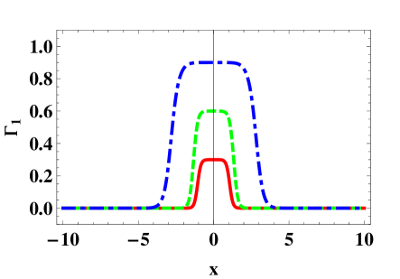
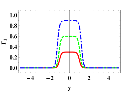
Figure 1: The constitutive parameters $\gamma_{22}$ and $\Gamma_{1}$ plotted versus $x$ for $y=z=0$, and versus $y$ for $x=z=0$. Parameter values: $\sigma=5$, $R=1$ and $v^{\prime}_{s}=0.9$ (blue, broken dashed curves), $0.6$ (green, dashed curves) and $0.3$ (red, solid curves).

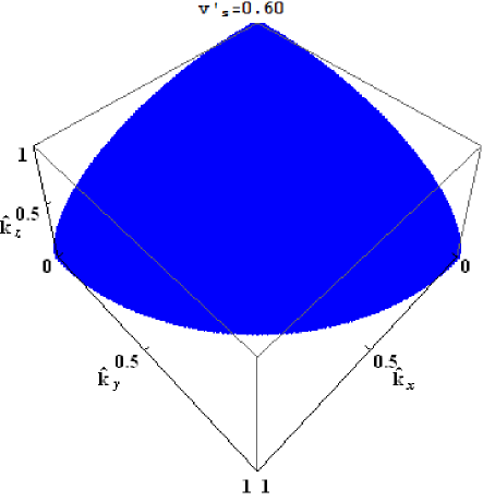
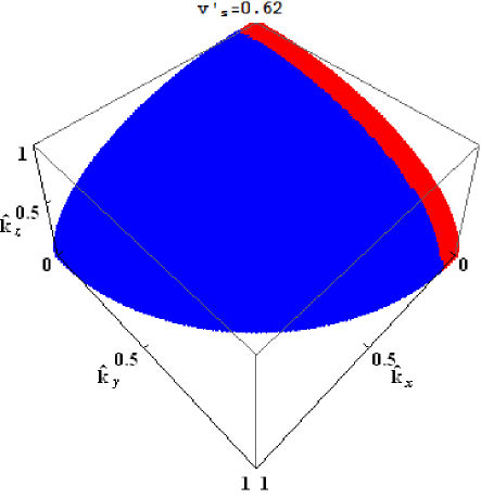
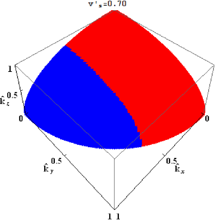
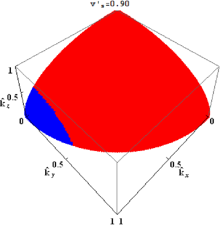
Figure 2: Maps illustrating the directions of $\hat{\underline{k}}=\underline{k}/k=\hat{k}_{x}\,\hat{\underline{x}}+\hat{k}_{y}\,\hat{\underline{y}}+\hat{k}_{z}\,\hat{\underline{z}}$ for which $\mbox{Im}\left\{k\right\}=0$ (blue) and $\mbox{Im}\left\{k\right\}\neq 0$ (red), at the coordinate origin for $v^{\prime}_{s}\in\left\{0.60,0.62,0.70,0.90\right\}$. Parameter values: $\sigma=5$ and $R=1$.

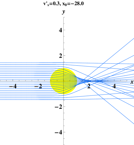
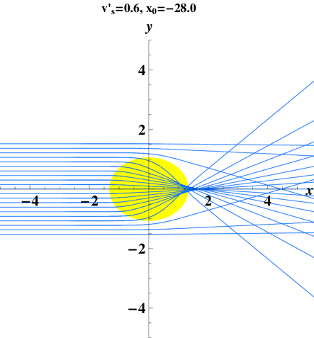
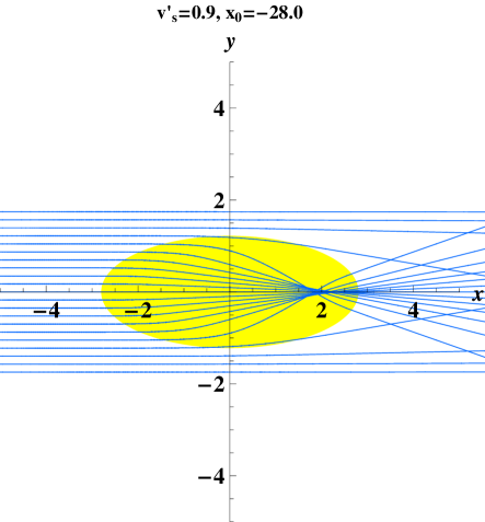
Figure 3: Trajectories for rays in the $xy$ plane, initially parallel to the $x$ axis and equally spaced. That is, $\underline{r}(0)=x_{0}\,\hat{\underline{x}}+y_{0}\,\hat{\underline{y}}$ with fixed $x_{0}=-28$ and $-1.5\,a_{m}<y_{0}<1.5\,a_{m}$, $\underline{k}(0)=\hat{\underline{x}}$ and $v^{\prime}_{s}\in\left\{0.3,0.6,0.9\right\}$. Parameter values: $\sigma=5$ and $R=1$.

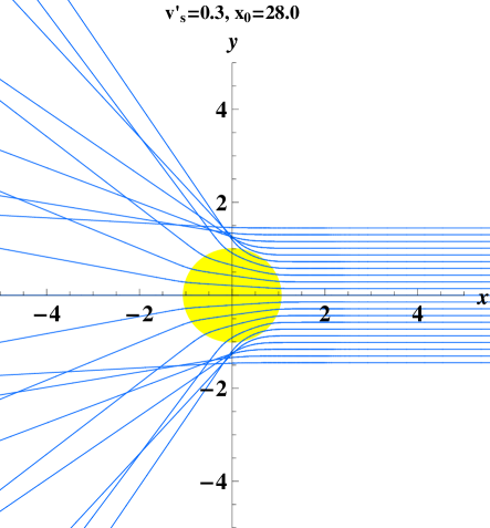
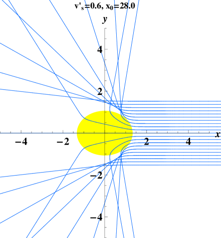
Figure 4: As Fig. 3 except that $x_{0}=28$ and $\underline{k}(0)=-\hat{\underline{x}}$.

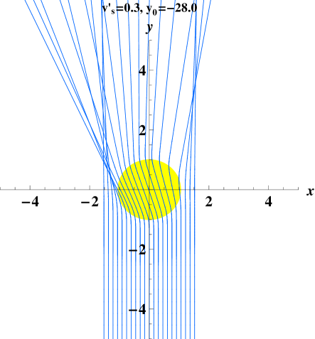
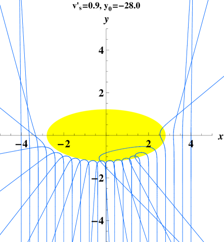
Figure 5: As Fig. 3 except that $\underline{r}(0)=x_{0}\,\hat{\underline{x}}+y_{0}\,\hat{\underline{y}}$ with $-1.5\,a_{M}<x_{0}<1.5\,a_{M}$ and fixed $y_{0}=-28$, and $\underline{k}(0)=\hat{\underline{y}}$

.

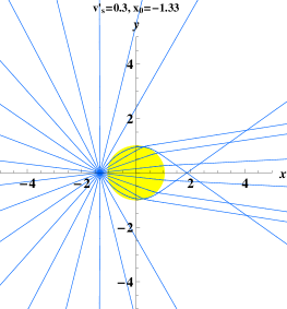
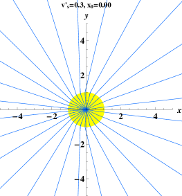
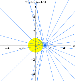
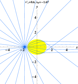
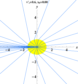
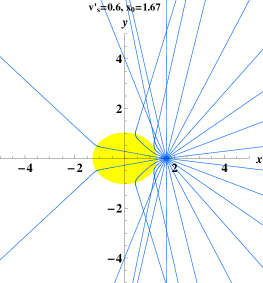
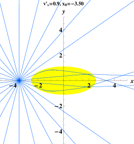
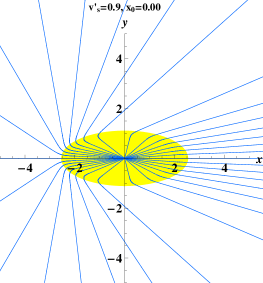
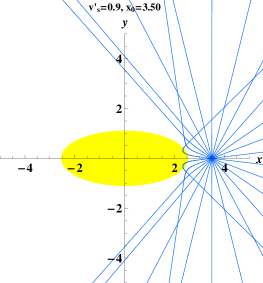
Figure 6: Trajectories for rays in the $xy$ plane, emanating from sources on the $x$ axis, i.e., $\underline{r}(0)=x_{0}\,\hat{\underline{x}}$, at equally spaced angular directions of $\underline{k}(0)$, for $v^{\prime}_{s}\in\left\{0.3,0.6,0.9\right\}$. Parameter values: $\sigma=10$ and $R=1$.

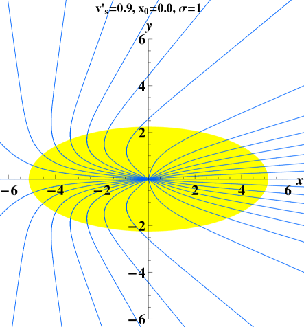
Figure 7: As Fig. 6 except that $v^{\prime}_{s}=0.9$ and $\sigma\in\left\{1,25\right\}$.

References

• [1] Smolyaninov I I 2011 Metamaterial ‘multiverse’ J Opt 13 024004
• [2] Skrotskii G V 1957 The influence of gravitation on the propagation of light Soviet Phys.–Dokl. 2 226–229
• [3] Plébanski J 1960 Electromagnetic waves in gravitational fields Phys. Rev. 118 1396–1408
• [4] Schleich W and Scully M O 1984 General relativity and modern optics New Trends in Atomic Physics Eds Grynberg G and Stora R (Amsterdam: Elsevier) pp.995–1124
• [5] Smolyaninov I I 2003 Surface plasmon toy model of a rotating black hole New J. Phys. 5 147
• [6] Mackay T G and Lakhtakia A 2010 Towards a metamaterial simulation of a spinning cosmic string Phys. Lett. A 374 2305–2308
• [7] Li M, Miao R–X and Pang Y 2010 Casimir energy, holographic dark energy and electromagnetic metamaterial mimicking de Sitter Phys. Lett. B 689 55–59
• [8] Li M, Miao R–X and Pang Y 2010 More studies on metamaterials mimicking de Sitter space Opt. Express 18 9026–9033
• [9] Greenleaf A, Kurylev Y, Lassas M and Uhlmann G 2009 Cloaking devices, electromagnetic wormholes, and transformation optics SIAM Rev. 51 3–33
• [10] Alcubierre M 1994 The warp drive: hyper-fast travel within general relativity Class. Quantum Grav. 11 L73–L77
• [11] Clark C, Hiscock W A and Larson S I 1999 Null geodesics in the Alcubierre warp-drive spacetime: the view from the bridge Class. Quantum Grav. 16 3965–3972
• [12] Natário J 2002 Warp drive with zero expansion Class. Quantum Grav. 19 1157–1166
• [13] Pfenning M J and Ford L H 1997 The unphysical nature of ‘warp drive’ Class. Quantum Grav. 14 1743–1752
• [14] Van Den Broeck C 1999 A ‘warp drive’ with more reasonable total energy requirements Class. Quantum Grav. 16 3973–3980
• [15] Lobo F S N and Visser M 2004 Fundamental limitations on warp drive spacetimes Class. Quantum Grav. 11 5871–5892
• [16] Hawking S W 1975 Particle creation by black holes Commun. Math. Phys. 43 199–220
• [17] Safonova M, Torres D F and Romero G E 2001 Microlensing by natural wormholes: theory and simulations Phys. Rev. D 65 023001
• [18] McCall M W, Lakhtakia A and Weiglhofer W S 2002 The negative index of refraction demystified Eur. J. Phys. 23 353–359
• [19] Mackay T G and Lakhtakia A 2009 Negative refraction, negative phase velocity, and counterposition in bianisotropic materials and metamaterials Phys. Rev. B 79 235121
• [20] Shelby R A, Smith D R, and Schultz S 2001 Experimental verification of a negative index of refraction Science 292 77–79
• [21] Ziolkowski R W 2001 Superluminal transmission of information through an electromagnetic metamaterial Phys. Rev. E 63 046604
• [22] Ruppin R 2002 Electromagnetic energy density in a dispersive and absorptive material Phys. Lett. A 299 309–312
• [23] Chen H C 1983 Theory of Electromagnetic Waves (New York: McGraw–Hill)
• [24] Van Bladel J 1985 Electromagnetic Fields (Washington: Hemisphere)
• [25] Mackay T G, Lakhtakia A and Setiawan S 2005 Gravitation and electromagnetic wave propagation with negative phase velocity New J. Phys. 7 75
• [26] Lakhtakia A and Mackay T G 2006 Dyadic Green function for an electromagnetic medium inspired by general relativity Chin. Phys. Lett. 23 832–833
• [27] Kline M and Kay I W 1965 Electromagnetic Theory and Geometric Optics (New York: Interscience)
• [28] Sluijter M, De Boer D K and Urbach H P 2009 Ray-optics analysis of inhomogeneous biaxially anisotropic media J. Opt. Soc. Amer. A 26 317–329
• [29] Anderson T H, Mackay T G and Lakhtakia A 2010 Ray trajectories for a spinning cosmic string and a manifestation of self–cloaking Phys. Lett. A 374 4637–4641
• [30] Mackay T G and Lakhtakia A 2010 Electromagnetic Anisotropy and Bianisotropy: A Field Guide (Singapore: World Scientific)
• [31] Smolyaninov I I 2010 Metamaterial-based model of the Alcubierre warp drive $\mathsf{http://arxiv.org/abs/1009.5663}$
Refer to caption
Refer to caption
Refer to caption
Refer to caption