Component Selection in the Additive Regression Model

Abstract

Similar to variable selection in the linear regression model, selecting significant components in the popular additive regression model is of great interest. However, such components are unknown smooth functions of independent variables, which are unobservable. As such, some approximation is needed. In this paper, we suggest a combination of penalized regression spline approximation and group variable selection, called the lasso-type spline method (LSM), to handle this component selection problem with a diverging number of strongly correlated variables in each group. It is shown that the proposed method can select significant components and estimate nonparametric additive function components simultaneously with an optimal convergence rate simultaneously. To make the LSM stable in computation and able to adapt its estimators to the level of smoothness of the component functions, weighted power spline bases and projected weighted power spline bases are proposed. Their performance is examined by simulation studies across two set-ups with independent predictors and correlated predictors, respectively, and appears superior to the performance of competing methods. The proposed method is extended to a partial linear regression model analysis with real data, and gives reliable results.

Keywords: Additive model, nonparametric component, group variable selection, penalized splines, lasso, generalized cross-validation.

1 Introduction

Consider the additive regression model

$$Y_{i}=\alpha+\sum_{k=1}^{K}f_{k}(X_{ki})+\varepsilon_{i},$$ (1.1)

where $X_{ki}$ are the components of $X_{i}=(X_{1i},\ldots,X_{Ki})$, $Ef_{k}(X_{ki})=0$, $\{f_{k}(\cdot),~{}k=1,\ldots,K\}$ are unknown smooth functions, and $\{\varepsilon_{i}\}$ is a sequence of i.i.d random variables with a mean of 0 and a finite variance $\sigma^{2}$. This model was first proposed by Friedman and Stuetzle (1981), and has become a popular multivariate nonparametric regression model in practice. Hastie and Tibshirani (1990) gave a comprehensive review of this model and showed that it could be widely used in multivariate nonparametric modeling.

The additive model provides an approximation, with an additive structure, for multivariate nonparametric regression. There are at least two benefits of such an additive approximation. First, as every single individual additive component can be estimated using a univariate smoother in an iterative manner, the so-called “curse of dimensionality” that besets multivariate nonparametric regression is largely avoided. Stone (1985, 1986) theoretically confirmed this by showing that one can construct an estimator of $f$ that achieves the same optimal convergence rate for a general value of $K$ as for $K=1$. Second, the estimate of each individual component explains how the dependent variable changes with the corresponding independent variables; essentially, the simpler structure improves the interpretability of the model.

There are several methods available in the literature for fitting the additive model. These include the backfitting algorithm (Friedman and Stuetzle 1981; Buja, Hastie and Tibshirani 1989; Opsomer and Ruppert 1998), the smooth backfitting algorithm (Mammen, Linton and Nielsen 1999, Mammen and Park 2005, Nielsen and Sperlich 2005; Mammen and Park 2006; Yu, Park and Mammen 2008), marginal integration estimation methods (Tjøstheim and Auestad 1994; Linton and Nielsen 1995; Fan et al.. 1998), the Fourier series or wavelets approximation approach (Amato, Antoniadis and De Feis 2002; Amato and Antoniadis 2001; Sardy and Tseng 2004), the penalized B-splines method (Eilers and Marx 2002), among others.

To make the additive model more efficient, the search for a parsimonious version is clearly of importance. Although estimation has been intensively investigated, insignificant independent variables and function components increase the complexity of the model, which leads to a great computational burden and numerical unstability. Hence, deriving a method for obtaining estimations in a parsimonious additive model that still achieve an optimal convergence rate, as is the case with only one nonparametric component, is an interesting issue.

We use a real data example to demonstrate why selecting significant components and searching for a parsimonious additive model is of importance for statistical additive modeling. Fan and Peng (2004) used an additive model and penalized SCAD least-squares to analyze the employee dataset of the Fifth National Bank of Springfield based on data from 1995 (see Example 11.3 in Albright et al. 1999). The bank, whose name has since changed, was charged in court with paying its female employees substantially smaller salaries than its male employees. For each of its 208 employees, the dataset includes the following variables.

• EduLev: education level, a categorical variable with categories 1 (finished high school), 2 (finished some college courses), 3 (obtained a bachelor’s degree), 4 (took some graduate courses), 5 (obtained a graduate degree).

• JobGrade: a categorical variable indicating the current job level, the possible levels being 1-6 (6 is the highest).

• YrHired: the year that an employee was hired.

• YrBorn: the year that an employee was born.

• Gender: a categorical variable that takes the value “Female” or “Male”.

• YrsPrior: the number of years of work experience that employee had at another bank before working at the Fifth National Bank.

• PCJob: a dummy variable that takes the value of 1 if the empolyee’s current job is computer-related, and 0 otherwise.

• Salary: the current (year 1995) annual salary in thousands of dollars.

Based on the discussions of Lam and Fan (2008) and Zhang (2008), both YrsExp and Age should have a nonlinear relationship with “Salary”, and an additive model should be an appropriate model to fit the data. The $R^{2}$ is $0.8123$. In the model, the nonparametric components of Age and YrsExp are included. This is informally confirmed by Figure 1, which presents the estimated curves of “YrsExp” and “Age”, respectively. However, the estimated function $f_{1}(\mathrm{YrsExp})$ is not an increasing function. This is inconsistent with the general intuition that salary should increase with “YrsExp”. It is natural to explore the reasons behind this inconsistency. As we might suppose that “Age” and “YrsExp” will be strongly correlated, we may naturally ask whether the phenomenon regarding “YrsExp” is caused by inappropriately including insignificant variables or components in the model. To demonstrate the necessity of component selection, we manually remove one component to see what happens. That is, we consider two additive models, each of which includes either “Age” or “YrsExp”. We find that the model without the “Age” component has a larger $R^{2}(0.8144)$ than the model with both “Age” and“YrsExp” , and the model without the “YrsExp” component has a smaller $R^{2}$ value of $0.8052$. This indicates that we should keep “YrsExp” in the model. More importantly, from Figure 2, we can see that when the “Age” component is selected out, the estimated function of “YrsExp” is an increasing function of “YrsExp”, which fits the intuition. This also suggests that when insignificant components are selected out, the remaining components have a better explanatory power. As such, the means of automatically selecting the “Age” component out from the model is of importance, because we need to select out a nonparametric component rather than a variable that is observable. We thus need a new method to handle this modeling issue.

Figure 1: The estimated regression functions of “Age” or “YrsExp” respectively when both are included in the additive model.

Figure 2: The estimated regression functions of “Age” or “YrsExp” respectively when both are included in the respective additive model.

1.1 Goals of the paper

There have been some studies on variable selection in additive modeling. Smith and Kohn (1996) proposed a Bayesian approach to select significant variables. Chen and H$\ddot{a}$rdle (1995) used a simple threshold method to select significant independent variables for the additive model, in which the function components are estimated by the marginal integration method. Shively, Kohn and Wood (1999) proposed a hierarchical Bayesian approach to variable selection and function estimation that uses a data-driven prior, and estimated their functions by model averaging. Lin and Zhang (2006) penalized the norm of the two-order derivative of component functions to obtain sparse additive model in which the functions are estimated by using a smoothing spline technique. Ravikumar et al.. (2009) proposed a new method to produce sparse additive model based on the idea of group variable selection and nonnegative garrote variable selection. All of these methods involve decoupled smoothing and sparsity, and penalize the norm of the estimated additive component functions to produce a sparse additive model. Most are based on classical variable selection methods for linear models, and hence cannot select significant independent variables and estimate the components simultaneously. The statistical properties of the estimates are also difficult to analyze. Furthermore, these methods impose a large computational burden, especially when there are many nonparametric function components to be estimated.

Recently, some attempts have been made to resolve these problems in the additive models (see, for example, Meier, van de Geer and Bühlmann 2009 and Huang, Horowitz and Wei 2009). These methods are based on the B-spline and group variable selection techniques and are capable of estimating and selecting component functions simultaneously, even in high-dimension situations. However, the approach developed by Meier, van de Geer and Bühlmann (2009) seems to be unstable in the selection process, because it uses every observation as a knot, which results in much fluctuation. The method proposed by Huang, Horowitz and Wei (2009) does not provide optimal estimates for the component functions. This is well known problem with spline regression because the efficiency of the estimates depends on the number and the position of the knots.

In this paper, we propose a lasso-type spline method (LSM) for component selection and estimation. First, we use a penalized regression spline approximation to parametrize the nonparametric components in the additive model, and then consider the spline approximation as a group of variables for selection. It is worth mentioning that in our setting, the design matrix in each group is formed from the truncated power spline basis functions. Hence, there is a diverging number of strongly correlated variables in each group, which makes the study more complicated and difficult. Nevertheless, the estimate of every single function component achieves the same optimal convergence rate as that in univariate local adaptive nonparametric regression splines, and our final selected model is rather parsimonious. To make the LSM in stable in computation and able to adapt its estimates to the level of smoothness of the component function, weighted penalized regression splines method and projected weighted penalized regression splines method are proposed. The two-stage estimation is obtained by using one-dimensional non-parametric techniques to refine the estimates in the first stage, which serve as initial approximations for the additive components. Our proposed procedure depends on only one parameter, which controls both prediction error and misclassification error. Hence, to a certain degree, it reduces the computational burden and attains computational stability. Simulation results illustrate that the method is superior in a set-up with independent predictors, and is comparable when the predictors are correlated.

The outline of the remainder of this paper is as follows. In Section 2, we describe our new method, study its asymptotic properties, and propose an approximation algorithm. In section 3, simulations and a real data application are presented to illustrate the performance of the proposed method. A brief conclusion and discussion are given in Section 4. The technical details of the proof are relegated to Section 5.

2 Methodology

2.1 Penalized regression splines

As the components in the additive model are unobservable nonparametric functions, it is impossible to perform selection directly, and an approximation is needed. To this end, we first examine the univariate nonparametric regression model with only one independent variable as a basis for our method.

$$Y_{i}=m_{0}(X_{i})+\epsilon_{i},~{}i=1,\ldots,n,$$

where $X_{i}$ is in $[0,~{}1]$. Mammen and Van de Geer (1997) proposed the use of the total variation $TV(m_{0}^{(p-1)})$ of the function $m_{0}(\cdot)$ as a penalty and to minimize the following penalized sum of the squared residuals to obtain the estimation of $m_{0}(\cdot)$,

$$F_{p,\lambda}=\sum_{i=1}^{n}(Y_{i}-m(X_{i}))^{2}+\lambda TV(m^{(p-1)}).$$

As with the smoothing spline, Mammen and Van de Geer (1997) proved that the minimizer of this equation falls into the spline space such that the estimate of $m_{0}(\cdot)$ itself is also a spline function. They also showed that the estimate of $m_{0}(\cdot)$ has some good asymptotic properties, such as local adaption and an optimal convergence rate.

To implement their idea, consider the following spline space $\mathcal{S}(p,\mbox{\boldmath$t$})$ with knots

$$\mbox{\boldmath$t$}=\{0=t_{0}<t_{1}<\ldots<t_{k+1}=1\}.$$

For $p\geq 2$, ${\cal S}(p,\mbox{\boldmath$t$})$ is defined as

$${\cal S}(p,\mbox{\boldmath$t$})=\{s(x)\in C^{p-2}[0,1]{~{}\rm where~{}}s(x)~{}~{}{\rm is~{}a~{}polynimial~{}of~{}the~{}order~{}}p{\rm~{}on~{}each~{}subinterval~{}}[t_{i},t_{i+1}]\}.$$

When $p=1$, ${\cal S}(p,\mbox{\boldmath$t$})$ is the set of step functions with jumps at the knots.

It is known that the space ${\cal S}(p,\mbox{\boldmath$t$})$ is a $k+p$ dimensional linear function space, and that the truncated power function series

$$\textbf{X}_{x}=\{1,x,x^{2},\ldots,x^{p-1},(x-t_{1})_{+}^{p-1},\ldots,(x-t_{k})_{+}^{p-1}\}$$

forms its basis (see de Boor, 1978). Thus, if the number of knots $k$ is sufficiently large, then we can approximate $m_{0}(x)$ by a spline function with the form

$$m(x,\mbox{\boldmath$\beta$})=\textbf{X}_{x}\mbox{\boldmath$\beta$}=\beta_{0}+\beta_{1}x+\ldots+\beta_{p-1}x^{p-1}+\sum_{i=1}^{k}\beta_{p+i-1}(x-t_{i})_{+}^{p-1}.$$ (2.1)

Note that

$$TV(m^{(p-1)}(x,\mbox{\boldmath$\beta$}))=\sum_{i=1}^{k}|m^{(p-1)}(t_{i},\mbox{\boldmath$\beta$})-m^{(p-1)}(t_{i-1},\mbox{\boldmath$\beta$})|=(p-1)!\sum_{i=1}^{k}|\beta_{p-1+i}|.$$

By minimizing

$$\min_{\mbox{\boldmath$\beta$}}\sum_{i=1}^{n}(Y_{i}-m(x_{i},\mbox{\boldmath$\beta$}))^{2}+\lambda\sum_{i=1}^{p}|\beta_{p-1+i}|,$$ (2.2)

we can obtain an estimate $m(x,\hat{}\mbox{\boldmath$\beta$})$ for the function $m_{0}(\cdot)$.

2.2 Component selection for the additive model

We now return to the additive regression model

$$Y_{i}=\alpha+\sum_{k=1}^{K}f_{k}(X_{ki})+\varepsilon_{i},~{}~{}i=1,\ldots,n.$$

For every function component, we assume that $Ef_{k}(\cdot)=0,~{}k=1,\ldots,K$, is approximated by the spline function

$$f_{k}^{*}(x)=\beta_{k0}+\beta_{k1}x+\ldots+\beta_{k(p-1)}x^{p-1}+\sum_{j=1}^{p_{k}}\beta_{k(p_{k}-1+p)}(x-t_{kj})_{+}^{p-1};$$ (2.3)

where $\{t_{kj},~{}j=1,\ldots,p_{k}\}$ is the series of knots for the $k$th function component.

For any $k$, let $\{B_{kj}(\cdot),~{}j=1,\ldots,p_{k}\}$ be the spline bases (note that although the number of bases should be $p_{k}+p-1$, for convenience, we still denote it as $p_{k}$). The additive model can then be approximated by the following linear model.

$$Y_{i}=\alpha^{*}+\sum_{k=1}^{K}\Big{(}\sum_{j=1}^{p_{k}}\beta_{kj}B_{kj}(X_{ki})\Big{)}+\varepsilon_{i},~{}i=1,\ldots,n.$$ (2.4)

For any $k$ with $1\leq k\leq K$, the basis series $B_{kj}(\cdot)$, $j=1,\ldots,p_{k}$ can be regarded as a natural group of variables in the foregoing linear model, and the group variable selection can be used to estimate $\beta_{kj}$ and to select the grouped variables. We combine the hierarchical LASSO method (Zhou and Zhu’s 2007), the group bridge approach (Huang et al.. 2009), and the ideas of Mammen and Van de Geer (1997) and propose the criterion

$$\min_{\alpha^{*},~{}\beta_{kj}}\sum_{i=1}^{n}\left\{Y_{i}-\alpha^{*}-\sum_{k=1}^{K}\sum_{j=1}^{p_{k}}\beta_{kj}B_{kj}(X_{ki})\right\}^{2}+\lambda\sum_{k=1}^{K}\sqrt{|\beta_{k1}|+|\beta_{k2}|+\ldots+|\beta_{kp_{k}}|}.$$

to select the groups. That is, we simultaneously to select the significant components, and estimate the parameters $\beta_{kj}$.

However, this linear approximation does not mean that the problem is exactly identical to the case in the classical linear model. First, to make a good approximation of the function $f_{k}(\cdot)$, $p_{k}$, the number of basis functions in the spline approximation, must be sufficiently large, and theoretically, increases with the sample size $n$. Thus, even when $K$, the number of function components, is of a moderate size, the linear structure derived has a diverging number of predictors if we do want to regard the model as linear. Second, the grouped variables $B_{kj}(\cdot),j=1,\ldots,p_{k}$, are all related to the variable $X_{k}$, and are thus strongly correlated, especially when the power basis functions are used. Third, distinct from Zhou and Zhu (2007), in our setup, the estimation accuracy of the whole function, rather than the estimation accuracy of a particular coefficient, is of interest and importance. Thus, as the objective here is to find a good approximation of each function component, the asymptotical results obtained by Zhou and Zhu (2007), and Huang et al.. (2009) can not be directly applied to the additive model.

2.3 Asymptotic theory

To study the asymptotic behavior of the model, we first consider a more general situation. Let $\mathscr{F}$ be a class of functions on $[0,1]$. For a linear subspace $\mathscr{F}_{n}$ of $\mathscr{F}$, we consider a penalty $\mathcal{P}:\mathscr{F}_{n}\to[0,\infty)$ that satisfies

$$\mathcal{P}(f_{1}+f_{2})\leq\mathcal{P}(f_{1})+\mathcal{P}(f_{2}),\quad f_{1},f_{2}\in\mathscr{F}_{n},$$

and

$$\mathcal{P}(\alpha f)\leq|\alpha|\mathcal{P}(f),\quad f\in\mathscr{F}_{n},\alpha\in\mathbf{R}.$$

Consider the additive model (1.1) with $f_{k}\in\mathscr{F},k=1,\ldots,K.$ For a tuning variable $\lambda_{n}$, $\hat{f}_{k},k=1,\ldots,K$ are estimated by minimizing the penalized sum of squares over $\mathscr{F}^{K}_{n}$:

$$\{\hat{f}_{1},\ldots,\hat{f}_{k}\}=\mbox{arg}\min\limits_{f_{1},\ldots,f_{K}\in\mathscr{F}_{n}}\left\{\frac{1}{n}\sum\limits_{i=1}^{n}\left(Y_{i}-\alpha-\sum\limits_{k=1}^{K}f_{k}(x_{i})\right)^{2}+\lambda_{n}\sum\limits_{k=1}^{K}\mathcal{P}^{\frac{1}{2}}(f_{k})\right\}.$$

Write $\mathscr{F}_{n}(1)=\{f\in\mathscr{F}_{n};\mathcal{P}\leq 1\}$. For a subset $\mathscr{A}$ of $\mathscr{F}$, we denote the $\delta$ entropy of $\mathscr{A}$ by $\log N_{2}(\delta,\|\cdot\|_{n},\mathscr{A})$. This is the logarithm of the minimal number of balls of a radius $\delta$ covering $\mathscr{A}$, where $\|\cdot\|_{n}$ is the $L_{2}$-norm with respect to the empirical probability measure of $x_{i}$ $i=1,\ldots,n$ with the form $\parallel g\parallel_{n}^{2}=\frac{1}{n}\sum_{i=1}^{n}g^{2}(x_{i}).$ To obtain the required result, we must first assume the following condition first.

Condition 1    The errors $\varepsilon_{1},\varepsilon_{2},\ldots,\varepsilon_{n}$ are independent, with $E\varepsilon_{i}=0,$ and have subgaussian tails. That is, there exist some positive $\beta$ and $\Gamma$ such that

$$\mbox{E}[\exp(\beta\varepsilon_{i}^{2})]\leq\Gamma\leq\infty,~{}~{}~{}~{}\mathrm{for}~{}i=1,~{}\ldots,~{}n.$$

Theorem 1.

Assume that Condition 1 holds. Let $c_{n}$ be a positive number sequence such that for the functions $f_{k,n},k=1,\ldots K$ in $\mathscr{F}_{n}$ we have

$$\|f_{k,n}-f_{k}\|_{n}=O(n^{-{1/(2+w)}}c_{n}^{w/{(2+w)}})\quad\mbox{and}\quad\mathcal{P}(f_{k,n})\leq c_{n},\ k=1,\ldots,K.$$ (2.6)

Let $\lambda_{n}=Cn^{-2/(2+w)}c_{n}^{1/2-(2-w)/(2+w)}.$ Furthermore, assume that for some $C>0$ and $0<w<2$, the following entropy bound condition is satisfied.

$$\log N_{2}(\delta,\|\cdot\|_{n},\mathscr{F}_{n}(1))\leq C\delta^{-w}\quad\mbox{for all}\ \delta>0.$$ (2.7)

We then have

$$\|\hat{f}_{k}-f_{k}\|_{n}=O_{p}(n^{-1/(2+w)}c_{n}^{w/(2+w)}),\quad\mbox{and}\quad\mathcal{P}(\hat{f}_{k})=O_{p}(c_{n}).$$

From (2.3)—(2.5), we can define the penalty functional as the $L_{1}$ norm of the coefficients for the spline approximation $f^{\ast}_{k}(\cdot)$, that is,

$$\mathcal{P}(f_{k}^{*})=\sum_{k=1}^{p+p_{k}-1}|\beta_{k}|.$$

In fact, this gives $\mathcal{P}(f_{k}^{*})=\sum_{k=0}^{p-1}|\beta_{k}|+(p-1)!\cdot\mathrm{TV}(f_{k}^{*(p-1)})$, where $\mathrm{TV}$ denotes the total variation. We obtain the following result for the entropy of the total variation space.

Proposition 1.

Define $\mathscr{F}_{n}(1)=\{f\in\mathscr{F}_{n}:\mathcal{P}(f)=\sum\limits_{k=1}^{K}\mathcal{P}(f_{k})\leq 1\}$. There then exists a constant $M>0$ such that

$$\log N_{2}(\delta,\|\cdot\|_{n},\mathscr{F}_{n}(1))\leq M\delta^{-1/p}.$$ (2.8)

To state our results for the asymptotic behavior of the penalized least-squares estimate (2.5), we need some further conditions.
Condition 2 For any $j$

$$\max_{1\leq i\leq k_{j}}|h_{ji+1}-h_{ji}|=o(k_{j}^{-1}),~{}~{}\frac{\max_{1\leq i\leq k_{j}}h_{ji}}{\min_{1\leq i\leq k_{j}}h_{ji}}\leq M,$$

where $h_{i}^{j}=t_{ji}-t_{ji-1}$, $k_{j}$ is the number of knots, and $M>0$ is a predetermined constant.

Theorem 2.

Assume that $f_{k}\in\mathscr{F},k=1,2,\ldots,K$, and that the total variation of its $(p-1)$-th derivative is bounded. Let $\lambda_{n}=Cn^{-\frac{2p}{2p+1}}$, where $C$ is a large constant. Then, under Conditions 1 and 2, we have

$$\parallel\hat{f}_{k}-f_{k}\parallel_{n}=O_{p}(n^{-\frac{p}{1+2p}})$$ (2.9)

for $\min\limits_{1\leq k\leq K}p_{k}>n^{\frac{1}{2p+1}}$.

2.4 Computation

2.4.1 Algorithms

The penalty function in (2.2) can be regarded as nonconcave. Hence, the quadratic approximation method and the iterative algorithm proposed by Fan and Li (2001) can be used to define estimates of the coefficients. First, consider the derivative of penalty function for $\beta_{kj}$. Let $\mathscr{P}(\mbox{\boldmath$\beta$}_{k})=\sqrt{|\beta_{k1}|+\ldots+|\beta_{kp_{k}}|}$. This gives

$$\mathscr{P}^{\prime}(\beta_{kj})=\frac{\lambda\cdot{\rm sgn}(\beta_{kj})}{\sqrt{|\beta_{k1}|+\ldots+|\beta_{kp_{k}}|}}=\frac{\lambda\cdot\beta_{kj}}{|\beta_{kj}|\sqrt{|\beta_{k1}|+\ldots+|\beta_{kp_{k}}|}}.$$ (2.10)

To simplify the notation, we rewrite (2.2) in matrix form as

$$(\textbf{Y}-\mbox{\boldmath$\alpha$}-\textbf{X}\mbox{\boldmath$\beta$})^{2}+\lambda\mathscr{P}(\mbox{\boldmath$\beta$}),$$ (2.11)

where $\textbf{X}=(X_{1},X_{2},\ldots,X_{n})^{T}$,

$$X_{i} = \{B_{11}(X_{1i}),\ldots,B_{1p_{1}}(X_{1i}),B_{21}(X_{2i}),\ldots,B_{2p_{2}}(X_{2i}),\ldots,B_{Kp_{K}}(X_{Ki})\}^{T}$$

$$\triangleq \{1,X_{\beta_{11}i},\ldots,X_{\beta_{1p_{1}}i},X_{\beta_{21}i},\ldots,X_{\beta_{2p_{2}}i},\ldots,X_{\beta_{Kp_{K}}i}\}^{T}$$

and $\mathscr{P}(\mbox{\boldmath$\beta$})=\sum_{k=1}^{K}\mathscr{P}(\mbox{\boldmath$\beta$}_{k})$.

If $\mbox{\boldmath$\beta$}^{*}$ with nonzero coefficients $(\alpha^{*},\mbox{\boldmath$\beta$}_{1}^{*},\ldots,\mbox{\boldmath$\beta$}_{K}^{*})$ minimizes the equation (2.11), then the following equation is satisfied.

$$\mbox{\boldmath$\beta$}^{*}=(\textbf{X}_{\mbox{\boldmath$\scriptstyle\beta$}^{*}}^{T}\textbf{X}_{\mbox{\boldmath$\scriptstyle\beta$}^{*}}+\Sigma_{\lambda}(\mbox{\boldmath$\beta$}^{*}))^{-1}\textbf{X}_{\mbox{\boldmath$\scriptstyle\beta$}^{*}}^{T}\textbf{Y},$$ (2.12)

where $\textbf{X}_{\mbox{\boldmath$\scriptstyle\beta$}^{*}}=(X_{1}^{*},X_{2}^{*},\ldots,X_{n}^{*})^{T}$, and

$$X_{i}^{*}=\{1,X_{\beta_{11}^{*}i},\ldots,X_{\beta_{Kp_{K}}^{*}i}\}^{T},$$

and

$$\Sigma_{\lambda}(\mbox{\boldmath$\beta$}^{*})=\mbox{diag}\{0,\mathscr{P}^{\prime}(\mbox{\boldmath$\beta$}_{1}^{*})/{\mbox{\boldmath$\beta$}_{1}^{*}},\ldots,\mathscr{P}^{\prime}(\mbox{\boldmath$\beta$}_{K}^{*})/{\mbox{\boldmath$\beta$}_{K}^{*}}\}.$$

Hence, as in Fan and Li (2001), given an initial value $\mbox{\boldmath$\beta$}_{0}$, (2.12) requires an iterative algorithm to update the estimate to $\mbox{\boldmath$\beta$}_{1}$ according to the following equation

$$\mbox{\boldmath$\beta$}_{1}=(\textbf{X}_{\mbox{\boldmath$\scriptstyle\beta$}_{0}}^{T}\textbf{X}_{\mbox{\boldmath$\scriptstyle\beta$}_{0}}+\Sigma_{\lambda}(\mbox{\boldmath$\beta$}_{0}))^{-1}\textbf{X}_{\mbox{\boldmath$\scriptstyle\beta$}_{0}}^{T}\textbf{Y}.$$

Fan and Li (2001) suggested that this iterative step is similar to the one-step MLE if the initial value is sufficiently good. If a reasonable initial value of $\beta$ is selected, then our algorithm should converge within a few steps.

2.4.2 Tuning parameter selection

The tuning parameter $\lambda$ is very important for estimating $\beta$. Fan and Li (2001) proposed using generalized cross-validation to select $\lambda$. Let $\hat{\mbox{\boldmath$\beta$}}(\lambda)$ be the estimate of $\beta$ with the tuning parameter $\lambda$. The generalized cross-validation statistic is defined as

$$\mbox{GCV}(\lambda)=\frac{1}{n}\frac{\parallel\textbf{Y}-\textbf{X}_{\hat{\mbox{\boldmath$\scriptstyle\beta$}}(\lambda)}\hat{\mbox{\boldmath$\beta$}}(\lambda)\parallel^{2}}{\{1-e(\lambda)/n\}^{2}}$$ (2.13)

and

$$\hat{\lambda}={\rm argmin}_{\lambda}\{\mbox{GCV}(\lambda)\},$$

where $e(\lambda)={\rm trace}[P_{X}(\hat{}\mbox{\boldmath$\beta$}(\lambda))]$, $P_{X}(\hat{}\mbox{\boldmath$\beta$})=\textbf{X}_{\hat{\mbox{\boldmath$\scriptstyle\beta$}}}(\textbf{X}^{T}_{\hat{\mbox{\boldmath$\scriptstyle\beta$}}}\textbf{X}_{\hat{\mbox{\boldmath$\scriptstyle\beta$}}}+\Sigma_{\lambda}(\hat{}\mbox{\boldmath$\beta$}))^{-1}\textbf{X}_{\hat{\mbox{\boldmath$\scriptstyle\beta$}}}^{T}$.

According to Wang, Li, and Tsai (2007), the log(GCV) is very similar to the traditional model selection criterion AIC. Although AIC is an efficient selection criterion that selects the best finite-dimensional candidate model in terms of prediction accuracy, it is not a consistent selection criterion because it does not select a correct model with a probability approaching 1 as the sample size goes to infinity. However, for our proposed method the number of knots, or the dimension of $\beta$ is very large and increases with the sample size $n$, and thus an adjustment for such a criterion is necessary. Accounting for the effect of dimensionality to correctly select the significant variables, we suggest using the inflated factor for GCV. A modified generalized cross-validation(MGCV) is defined as

$$\mbox{MGCV}(\lambda)=\frac{1}{n}\frac{\parallel\textbf{Y}-\textbf{X}\hat{\mbox{\boldmath$\beta$}}(\lambda)\parallel^{2}}{\{1-\gamma e(\lambda)/n\}^{2}}$$ (2.14)

where $\gamma$ is the inflated factor. When $\gamma=1$, the MGCV is no different from the GCV proposed by Fan and Li (2001). Based on our experience and the discussions of Luo and Wahba (1997) and Friedman and Silverman (1989), we suggest selecting $\gamma$ within the interval $(1.2,3)$ as an extra penalty.

2.5 Further Considerations

2.5.1 Weighted penalized regression splines method

Our method is based on the power spline regression. It is well known that the power spline regression is not stable in computation because of a strong correlation between power bases, and many base functions are related to only a few observations. To make our numerical results more stable, we weight the power spline base for every component function as

$$\mathbf{X}^{*w}=\mathbf{X}^{*}\times\mathbf{W},$$

where $\mathbf{W}^{2}=\mbox{diag}\{(\mathbf{X}^{*T}\mathbf{X}^{*}/n)^{-1}\}$ and $\mathbf{X}^{*}$ is given in (2.12). (2.11) can then be rewritten as

$$(\textbf{Y}-\mathbf{X}^{*wT}\mbox{\boldmath$\beta$}^{*w})^{2}+\lambda\mathscr{P}(\mbox{\boldmath$\beta$}^{*w}).$$

By some elementary calculations, it is easy to determine that when all of the components of $\mathbf{X}^{*w}$ are independent, the variance of the least-squares estimate of $\mbox{\boldmath$\beta$}^{*w}$ should be of the order $1/n$. Also, when the sample points $X_{ki},i=1,\ldots,n$ are equally spaced, our method is equivalent to transferring the power base spline approximation to a B-spline approximation with an $L_{1}$-norm penalty of a linear combination of the coefficients in the B-spline approximation. Furthermore, as the variance of the least-squares estimate of $\mbox{\boldmath$\beta$}^{\ast}$ is of the order $1/n$, as to the wavelet approximation (Donoho and Johnstone 1994), the universal threshold $\sqrt{\log n/n}$ can be used to penalize each coefficient. In other words, the tuning parameter can be searched within a small interval with the length $O(\sqrt{\log n/{n}})$. These modifications result in a stable final penalized component function estimate.

2.5.2 Projected weighted penalized regression splines method

To make our final estimated model parsimonious and easy to interpret, in addition to selecting significant component functions, we also suggest the following procedure for the component estimation. Note that the power spline approximation (see the definition of $\mathbf{X}_{x}$ above (2.1)) expands the component function as the sum of a polynomial and a linear combination of truncated power base functions. Divide $\mathbf{X}^{*w}$ by $(\mathds{1},B^{*w}_{1},\ldots,B^{*w}_{k},\ldots,B^{*w}_{K})$, with $B^{*w}_{k}$ being the block from the $(2+\sum\limits_{l=1}^{k-1}p_{l})$-th column to the $(1+\sum\limits_{l=1}^{k}p_{l})$-th column in matrix $\mathbf{X}^{*w}$. Here, $\mathds{1}$ is an $n\times 1$ column vector in which all the elements are equal to 1. We then write $B^{*w}_{k}=(B^{*w}_{k1}\quad B^{*w}_{k2})$, where $B^{*w}_{k1}$ are the coefficients of the polynomial part and $B^{*w}_{k2}$ are the coefficients of the truncated power base functions. We regard these as two groups and then penalize each group separately, which make it possible to adaptively estimate the component functions when they are actually polynomial functions without any great effect from the truncated power base functions. This provides a way of adaptively estimating the component functions if they are actually polynomial, and means that the estimation is adaptive to the level of smoothness of the component functions. This approach may result in a more parsimonious estimation than that obtained by the previous estimation algorithm. However, we note that the two groups are strongly correlated. To realize the approach and to make the algorithm more efficient, we consider the following empirical power base functions.

$$B^{*pw}_{k}=\{B^{*w}_{k1}\quad(I-P_{B^{*w}_{k1}})B^{*w}_{k2}\},$$

where $P_{B^{*w}_{k1}}$ is the project matrix from $B^{*w}_{k2}$ to $B^{*w}_{k1}$. This projection method is able to reduce the correlation between the two groups in the spline approximation. Let

$$\mathbf{X}^{pw}=(\mathds{1},B^{*pw}_{1},\ldots,B^{*pw}_{k},\ldots,B^{*pw}_{K}).$$

(2.11) can also be written as

$$(\textbf{Y}-\mathbf{X}^{*pw}\mbox{\boldmath$\beta$}^{*pw})^{2}+\lambda\mathscr{P}(\mbox{\boldmath$\beta$}^{*pw}_{1})+\lambda\mathscr{P}(\mbox{\boldmath$\beta$}^{*pw}_{2}),$$

where $\mathscr{P}(\mbox{\boldmath$\beta$}^{*pw}_{1})$ are the group penalty functions for the polynomial coefficients for all of the component additive functions and $\mathscr{P}(\mbox{\boldmath$\beta$}^{*pw}_{2})$ are the group penalty functions for the coefficients of the truncated power bases.

2.5.3 Two-stage estimation

When the dimension of the additive regression model is very high, selecting significant component functions becomes very difficult. The model selection and estimation may not be consistent, and the estimation procedure may also become unstable. To improve the estimation accuracy, we suggest a two-stage estimation approach. In the first stage, we use our proposed methods to select and estimate significant component functions as initial approximations of all of the selected components. Let

$$\mathcal{M}=\{k:f_{k}(X_{k})\mbox{\,\, selected to be significant based on our methods}\}$$

and denote the corresponding estimates by $\hat{f}^{0}_{k},\,k\in\mathcal{M}$. In the second stage, we obtain refined estimates as follows. For the $f_{s}(\cdot)$ selected in the first stage, define

$$Y^{\ast}_{i}=Y_{i}-\sum\limits_{k\in\mathcal{M},k\neq s}\hat{f}^{0}_{k}(X_{ki}),\,\,i=1,2,\ldots,n$$

and then estimate $f_{s}(X_{si})$ non-parametrically using the following model

$$Y^{\ast}_{i}=f_{s}(X_{si})+\varepsilon^{\ast}_{i},\,\,i=1,\ldots,n.$$

For this new model, we can again use the method applied in the first-stage estimation to obtain the final estimator of $f_{s}(X_{si})$.

3 Numerical studies

3.1 Simulations

We conduct simulations to examine the effectiveness of the proposed lasso-type spline method for component function selection and estimation in the additive regression model. The algorithm proposed in Section 2.4.1 is called the original lasso-type spline method (OLSM), that in Section 2.5.1 the weighted lasso-type spline method (WLSM), and that in Section 2.5.2 the projected weighted lasso-type spline method (PWLSM). We also compare the results with those obtained using the sparsity-smoothness penalty (SSP) approach recently proposed by Meier, van de Geer, and Bühlmann (2009) by using the R packages provided by the authors. For selection performance, we compute the true positive ratio (TPR) and false positive ratio (FPR); and for estimation accuracy, we compute the empirical prediction mean square error (MSE). Letting $\hat{f}_{k}$ be the estimator of $f_{k}$, MSE is defined as

$$\frac{1}{n}\sum\limits_{i=1}^{n}|\hat{f}_{k}(X_{ki})-f_{k}(X_{ki}))|^{2},$$

where $\{Y_{i},X_{1i},\ldots,X_{Ki}\}$ are the data points.

In the simulations, the sample size $n=400$ and a total of $100$ simulation runs are used. To reduce the computational burden, the knots are designed as follows. Let the number of knots be $k$. For each predictor $X_{i}$, the knots are selected to be the $[nj/k]$-th order statistics $\{X_{i([nj/k])},j=1,\ldots,k\}$ of $\{X_{j1},\ldots,X_{jn}\}$. Quadratic splines are used, which gives a total number of base functions with $K$ function components of $(2+k)K+1$. To check the sensitivity of the methods to the knot number selection, we tried the values $10,15,40$, and $60$ with a fixed $\lambda$, and found that the numerical results did not differ much. We thus posit that our proposed three procedures are insensitive to the initial knot number as long as it is sufficiently large. However, with a larger number knots, the computation time is grated and the performance is a little worse, as the computation may be less stable due to strongly correlated variables in the splines. We thus set $k$ at $15$ in the simulations. The penalty parameter $\lambda$ is found to be critical. We choose $\lambda$ by computing the MGCV criterion defined in (2.14) for a grid of $\alpha$ values and choosing the minimizer over the grid. The inflated factor $\gamma$ is taken to be $1.5$. The grid of $\lambda$ for all three proposed procedures has 100 values and satisfies the condition that the values of $\log_{10}(\lambda)$ are equally spaced between $-5$ and $2$. The sparsity-smoothness penalty approach (SSP) require teh selection of two parameters $\lambda_{1}$ and $\lambda_{2}$, where the former serves to control the sparsity and the latter the smoothness. Both parameters are chosen by using $100$ grid points for $\lambda_{1}$ and $15$ grid points for $\lambda_{2}$ in the spirit of Meier, van de Geer, and Bühlmann (2009). The simulation experiments are similar to those in Example 1 and Example 3 of Meier, van de Geer, and Bühlmann (2009). As our focus is on simultaneous selection and estimation, $K$ is chosen to be $50$ rather than an ultra-high dimension.

 Example 1.

(Covariates are independent). The data are generated from

$$Y=f_{1}(X_{1})+f_{2}(X_{2})+f_{3}(X_{3})+f_{4}(X_{4})+\sum\limits_{k=5}^{50}f_{k}(X_{k})+\varepsilon,$$

where

$$\begin{array}[]{rll}&f_{1}(x)=-\sin(2x),\mbox{\quad}f_{2}(x)=x^{2}-25/12,&f_{3}(x)=x,\\ &f_{4}(x)=\exp(-x)-2\sinh(5/2)/5,&f_{k}(x)=0,\mbox{\quad if \quad}k\geq 5,\end{array}$$

and $\varepsilon\sim N(0,1)$. The predictors are sampled from the uniform distribution of $(-2.5,2.5)$.

 Example 2.

(Covariates are correlated). The model is

$$Y=f_{1}(X_{1})+f_{2}(X_{2})+f_{3}(X_{3})+f_{4}(X_{4})+\sum\limits_{k=5}^{50}f_{k}(X_{k})+\varepsilon,$$

with

$$\begin{array}[]{rll}&f_{1}(x)=5x,\quad f_{2}(x)=3(2x-1)^{2},\quad f_{3}(x)=\frac{4\sin(2\pi x)}{2-\sin(2\pi x)},\\ &f_{4}(x)=0.6\sin(2\pi x)+1.2\cos(2\pi x)+1.8\sin^{2}(2\pi x)+2.4\cos^{3}(2\pi x)+3\sin^{3}(2\pi x),\\ &f_{k}(x)=0,\mbox{\quad if \quad}k\geq 5,\end{array}$$

and $\varepsilon\sim N(0,1.74)$. The covariates $X=(X_{1},\ldots,X_{K})$ are generated from

$$X_{k}=\frac{W_{k}+0.5U}{1+0.5},\quad k=1,\ldots,K,$$

where $W_{1},\ldots,W_{K}$ and $U$ are i.i.d uniform(0, 1). This provides a design with a correlation coefficient of $0.5$ between all of the covariates.

The simulation results are reported in Tables LABEL:table-ind and LABEL:table-cor. The median of the MSE and the robust standard deviation of the MSE (the ratio of the interquartile and the standard normal interquartile $(\Phi^{-1}(0.75)-\Phi^{-1}(0.25))$) are reported.“$\mbox{MSE}_{f_{k}}$” means the MSE value of the estimates for $f_{k}(\cdot)$, and “MSE” means the MSE for the full model. The row “SSP” shows the results of the SSP method developed by Meier, van de Geer, and Bühlmann (2009). The rows “OLSM”, “WLSM”, and “PWLSM” respectively summarize the results that are based on “oracle” (assuming that all of the functions are known except that to be estimated), “one-stage”, and “two-stage” estimates for the original lasso-type spline method, the weighted lasso-type spline method, and the projected weighted lasso-type method, respectively. The TPR and FPR results for each method are reported in Table LABEL:table-TP. The curve estimations for the component functions are respectively summarized in Figures 3—8.

[caption = Mean squared error (MSE) for Example 1 (the numbers in parentheses are the robust standard deviations estimations)., label= table-ind, pos=h]lccccccccc $\mbox{MSE}_{f_{1}}$ $\mbox{MSE}_{f_{2}}$ $\mbox{MSE}_{f_{3}}$ $\mbox{MSE}_{f_{4}}$ MSE SSP 0.122(0.189) 0.105(0.210) 0.105(0.189) 0.124(0.188) 1.358(0.277) Oracle 0.024(0.110) 0.013(0.108) 0.008(0.080) 0.028(0.126) 0.082(0.217) OLSM One-stage 0.530(0.142) 0.119(0.217) 0.190(0.217) 0.511(0.253) 1.357(0.295) Two-stage 0.526(0.145) 0.022(0.143) 0.035(0.188) 0.366(0.165) 0.949(0.267) Oracle 0.020(0.105) 0.013(0.111) 0.008(0.083) 0.027(0.128) 0.081(0.219) WLSM One-stage 0.479(0.292) 0.025(0.133) 0.052(0.204) 0.071(0.175) 0.615(0.338) Two-stage 0.040(0.592) 0.014(0.118) 0.013(0.093) 0.038(0.142) 0.141(0.575) Oracle 0.011(0.101) 0.015(0.112) 0.006(0.084) 0.024(0.130) 0.078(0.210) PWLSM One-stage 0.115(0.141) 0.016(0.115) 0.008(0.094) 0.042(0.158) 0.194(0.265) Two-stage 0.022(0.111) 0.016(0.125) 0.011(0.108) 0.027(0.146) 0.090(0.251)

[caption = Mean square error (MSE) for Example 2 (the numbers in parentheses are the robust standard deviations estimations)., label= table-cor, pos=h]lccccccccc $\mbox{MSE}_{f_{1}}$ $\mbox{MSE}_{f_{2}}$ $\mbox{MSE}_{f_{3}}$ $\mbox{MSE}_{f_{4}}$ MSE SSP 0.225(0.373) 0.430(0.624) 0.755(0.328) 3.020(0.580) 7.224(0.764) Oracle 0.025(0.116) 0.282(0.198) 0.047(0.148) 1.566(0.635) 3.127(0.795) OLSM One-stage 0.133(0.277) 0.594(0.139) 0.394(0.305) 2.315(0.611) 4.475(0.789) Two-stage 0.045(0.218) 0.589(0.181) 0.163(0.256) 1.696(0.621) 3.585(0.787) Oracle 0.018(0.110) 0.281(0.187) 0.050(0.154) 1.558(0.623) 3.112(0.780) WLSM One-stage 0.072(0.140) 0.470(0.412) 0.309(0.284) 1.880(0.623) 3.842(0.831) Two-stage 0.027(0.149) 0.312(0.464) 0.046(0.161) 1.574(0.631) 3.216(0.818) Oracle 0.025(0.112) 0.295(0.210) 0.055(0.156) 1.573(0.630) 3.178(0.778) PWLSM One-stage 0.066(0.124) 0.403(0.364) 0.195(0.212) 1.759(0.606) 3.590(0.784) Two-stage 0.022(0.134) 0.295(0.236) 0.052(0.159) 1.555(0.628) 3.176(0.760)

[caption = Median of the number of true positives (TP) and false positives (FP) (the numbers in parentheses are the standard robust deviations estimations)., label=table-TP, pos=h]lccccccccc TP FP SSP 4.000(0.000) 0.000(0.000) OLSM 3.000(0.000) 0.000(0.000) Example 1 WLSM 4.000(0.741) 0.000(0.000) PWLSM 4.000(0.000) 0.000(0.000) SSP 4.000(0.741) 0.000(0.741) OLSM 3.000(0.000) 1.000(1.483) Example 2 WLSM 4.000(0.741) 0.000(0.741) PWLSM 4.000(0.000) 1.000(0.741)

The results tabulated in Tables LABEL:table-ind and LABEL:table-TP and plotted in Figures 5 and 7 with independent covariates in Example 1 show the differences among the “oracle” cases and the OLSM, WLSM, and PWLSM cases to be nearly negligible. The MSE of the two-stage estimates is significantly smaller than that of the corresponding one-stage estimates and approximate that in the “oracle” case. Of all of these methods, the two-stage estimates of the PWLSM are superior to the others. The numbers of true positives and false positives for the PWLSM are the same as those of the SSP approach. However, the OLSM has a smaller number of true positives and the WLSM has a larger variation in true positives than the SSP, although the true positives for the WLSM is the same as that for the SSP. Figures 3, 5, and 7 show that the OLSM and WLSM may fail to select the first component function. This is because the first function is small in magnitude, and is easily selected out from the model due to the penalty. In contrast, the PWLSM always selects all of the non-zero component functions into the model, and the knots used in the spline basis are very sparse. Furthermore, the PWLSM selects the linear function (for example, the third panel on the top) as linear, whereas the SSP fails to do so. The PWLSM thus outperforms the other methods in this setting.

For the correlated covariate case in Example 2, the results presented in Tables LABEL:table-cor and LABEL:table-TP and Figures 4, 6 and 8) suggest that all of the “oracle” estimations perform similarly. Our proposed three LSMs all apparently improve on the method the SSP in terms of the MSE. The numbers of true positives and false positives for the WLSM are the same as those for the SSP. However, the PWLSM does not perform better in every respect, as it keeps selecting all of the true components at the expense of including a component that is slightly more noisy than the other insignificant components.

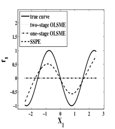
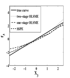
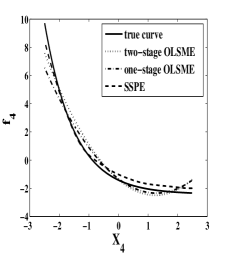
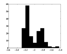
Figure 3: Estimation curves from the original Lasso-type spline method (OLSM) for Example 1. True functions $f_{j}$ and estimation curves $\hat{f}_{j}$ for the first four components of the simulation run that achieved the median of the MSE are presented. The pictures in the second row are histograms of the knots used in the one-stage OLSM estimation for the first four components, respectively.

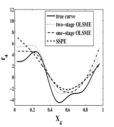
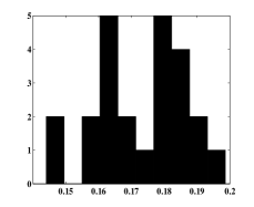
Figure 4: Estimation curves from the original Lasso-type spline method (OLSM) for Example 2. True functions $f_{j}$ and estimation curves $\hat{f}_{j}$ for the first four components of the simulation run that achieved the median of the MSE are presented. The pictures in the second row are histograms of the knots used in the one-stage OLSM estimation for the first four components, respectively.

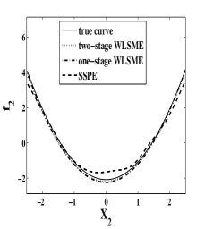
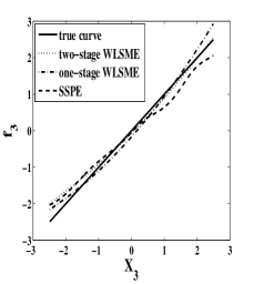
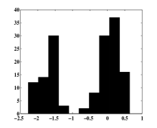
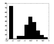
Figure 5: Estimation curves from the weighted Lasso-type spline method (WLSM) for Example 1. True functions $f_{j}$ and estimation curves $\hat{f}_{j}$ for the first four components of the simulation run that achieved the median of the MSE are presented. The pictures in the second row are histograms of the knots used in the one-stage WLSM estimation for the first four components, respectively.

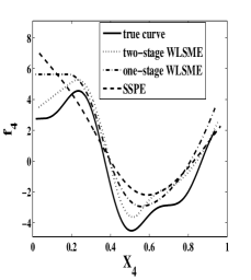
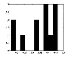
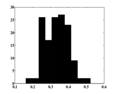
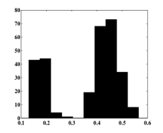
Figure 6: Estimation curves from the weighted Lasso-type spline method (WLSM) for Example 2. True functions $f_{j}$ and estimation curves $\hat{f}_{j}$ for the first four components of the simulation run that achieved the median of MSE are presented. The pictures in the second row are histograms of the knots used in the one-stage WLSM estimation for the first four components, respectively.

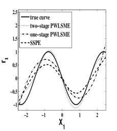
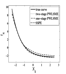
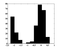
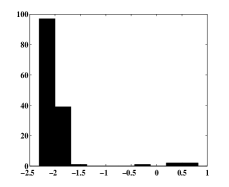
Figure 7: Estimation curves from the projected weighted Lasso-type spline method (PWLSM) for Example 1. True functions $f_{j}$ and estimation curves $\hat{f}_{j}$ for the first four components of the simulation run that achieved the median of the MSE are presented. The pictures in the second row are histograms of the knots used in the one-stage PWLSM estimation for the first four components, respectively.

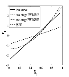
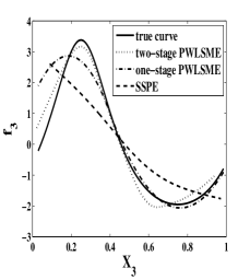
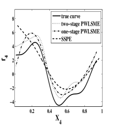
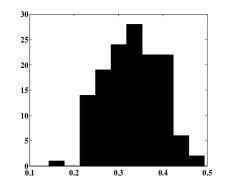
Figure 8: Estimation curves from the projected weighted Lasso-type spline method (PWLSM) for Example 2. True functions $f_{j}$ and estimation curves $\hat{f}_{j}$ for the first four components of the simulation run that achieved the median of the MSE are presented. The pictures in the second row are histograms of the knots used in the one-stage PWLSM estimation for the first four components, respectively.

3.2 Application

In this section, we give more details of the analysis of the dataset described in Section 1. As described, the dataset has been analyzed by Fan and Peng (2004) with the linear model and the additive model, respectively. We now use the method proposed in this paper to analyze the dataset and to make a comparison with the results of Fan and Peng (2004).

Similar to the approach of Fan and Peng (2004), we also move out the outliers and use the 199 remaining observations for our analysis. Consider the additive model

$$\mathrm{Salary} = \beta_{0}+\beta_{1}\mathrm{Female}+\beta_{2}\mbox{PCJob}+\sum\limits_{i=1}^{4}\beta_{2+i}\mathrm{Edu}_{i}+\sum\limits_{i=1}^{5}\beta_{6+i}\mathrm{JobGrd}_{i}$$ (3.1)

$$+f_{1}(\mathrm{YrsExp})+f_{2}(\mathrm{Age})+\varepsilon.$$

We use LASSO for the linear part and our method for the component function selection. The $2/17,3/17,\ldots,16/17$ sample quantiles of the variables “YrsExp” and “Age” are selected as knots, which gives 15 initial knots to estimate the component functions. Fan and Peng (2004) used only 5 knots to estimate each component function, whereas our method gives 20 more parameters to model data. Despite this, the computational complexity is not increased because the quadratic approximation algorithm can be easily implemented, and most of the knots will be removed in an iterative fashion by our component selection procedure. In line with Fan and Peng (2004) and the foregoing discussion, we first weight the “design matrix” such that the original least-squares estimate has the standard deviation of every estimate of the coefficients of the prediction variables and a truncated power basis function close to the order of $1/\sqrt{n}$. Two tuning parameters are then used to select the variables in the linear part and the component functions. MGCV with an inflation parameter of $1.5$ is used to select the tuning parameters. The results are reported in the fourth column (WLSM, see Section 3.1) of Table LABEL:table-data and in Figure 9.

Table LABEL:table-data shows that our method does not select the component function of “Age”. This is consistent with the result of SCAD-PLS for the linear model, which is reported in the second column of Table LABEL:table-data. The other estimates of the coefficients are similar to those obtained with the first three methods. The function of “YrsExp” is now estimated as an increasing function (see Figure 9). Only two spline bases, from among the 17 are selected to estimate the component function of “YrsExp”. Hence, the selected model is much simpler than the selected model derived with SCAD-PLS under the additive structure. The $R^{2}$ value in the fourth column for the WLSM is larger than that in the second or third column for SCAD-PLS. This means that, compared with the SCAD-PLS method for either the linear model or the additive model, our method provides a more reasonable estimation and selects a simpler model in this real data example.

[caption = Estimates and standard errors for the Fifth National Bank data., label=table-data, pos=h] rrcrcrcrcrcccccc Least-Squares SCAD PLS SCAD PLS WLSM Intercept 54.238(2.067) 55.835(1.527) 52.470(2.890) 55.820(1.437) Female -0.556(0.637) -0.624(0.639) -0.933(0.708) -0.693(0.656) PcJob 3.982 (0.908) 4.151(0.909) 2.851(0.640) 3.935(0.908) Ed1 -1.739(1.049) 0(—) 0(—) 0(—) Ed2 -2.866(0.999) -1.074(0.522) -0.542(0.265) -1.385(0.764) Ed3 -2.145(0.753) -0.914(0.421) 0(—) -1.180(0.601) Ed4 -1.484(1.369) 0(—) 0(—) 0(—) Job1 -22.954(1.734) -24.643(1.535) -22.841(1.332) -23.325( 1.561) Job2 -21.388(1.686) -22.818(1.546) -20.591(1.370) -21.494(1.580) Job3 -17.642(1.634) -18.803(1.562) -16.719(1.391) -17.440(1.602) Job4 -13.046(1.578) -13.859(1.529) -11.807(1.359) -12.536(1.542) Job5 -7.462(1.551) -7.770(1.539) -5.235(1.150) -6.477 (1.537) YrsExp 0.215(0.065) 0.193(0.046) —(—) —(—) Age 0.030(0.039) 0(—) —(—) 0(—) $R^{2}$ 0.8221 0.8176 0.8123 0.8182

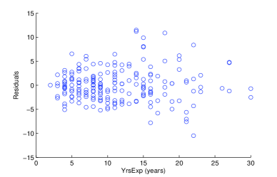
(a)	(b)

Figure 9: (a) Regression components $f_{1}$, and (b) Residuals versus Years Experience for the partial additive linear model by SCAD penalized least-squares (3.1).

4 Conclusion

In this paper, we propose a LASSO-type method for selecting nonparametric components in the additive regression model. We can use this method to simultaneously select and estimate components. Simulations show that for a high-dimensional additive model, the proposed methods can shrink the function components that correspond to the nonsignificant predictors exactly to zero and produce a parsimonious model. For an ultra-high dimensional additive model, we follow the idea of Fan et al. (2009) and use then SIS method to first reduce the ultra-dimension of the additive model to a high dimension, and then use our proposed method to select and estimate the significant components. Intuitively, it is possible to extend this idea to generalized additive models with binary response data or poisson data, or with a given link function. Research in this area is ongoing.

5 Proof of Theorems

Proof of Theorem 1: As $\mu=Ef_{0}(\textbf{X})$, a natural consistent estimate of $\mu$ is $\hat{\mu}=\frac{1}{n}\sum_{i=1}^{n}y_{i}$. Without loss of generality, assume that $\mu=0$. By the condition (2.6), there exist $f^{\ast}_{k,n}$ such that

$$\|f^{\ast}_{k,n}-f_{k}\|_{n}=O(n^{-1/(2+w)}c_{n}^{w/(2+w)})\quad\mbox{and}\quad\mathcal{P}(f^{\ast}_{k,n})\leq c_{n},\quad\mbox{for}\ k=1,\ldots,K.$$

Define $f_{n}^{\ast}=\sum\limits_{k=1}^{K}f_{k,n}^{\ast}\in\mathscr{F}_{n}$ that satisfies

$$\|f-f_{n}^{\ast}\|_{n}=\|\sum\limits_{k=1}^{K}f_{k}-\sum\limits_{k=1}^{K}f_{k,n}^{\ast}\|_{n}\leq\sum\limits_{k=1}^{K}\|f_{k}-f_{k,n}^{\ast}\|_{n}=O(n^{-1/(2+w)}c_{n}^{w/(2+w)})$$

and

$$\mathcal{P}(f_{n}^{\ast})=\sum\limits_{k=1}^{K}\mathcal{P}^{\frac{1}{2}}(f_{n,k}^{\ast})\leq K\cdot c^{\frac{1}{2}}_{n}.$$

By the definition of $\hat{f}_{n}$, we have

$$\frac{1}{n}\sum\limits_{i=1}^{n}(Y_{i}-\hat{f}_{n}(\mbox{\bf X}_{i}))^{2}+\lambda_{n}\mathcal{P}(\hat{f}_{n})\leq\frac{1}{n}\sum\limits_{i=1}^{n}(Y_{i}-f_{n}^{\ast}(\mbox{\bf X}_{i}))^{2}+\lambda_{n}\mathcal{P}(f^{\ast}_{n}),$$

and

$$\|\hat{f}_{n}-f_{n}^{\ast}\|^{2}_{n} \leq \lambda_{n}(\mathcal{P}(f_{n}^{\ast})-\mathcal{P}(\hat{f}_{n})+\frac{2}{n}\sum\limits_{i=1}^{n}\varepsilon_{i}(\hat{f}_{n}(\mbox{\bf X}_{i})-f_{n}^{\ast}(\mbox{\bf X}_{i}))$$

$$+ \frac{2}{n}\sum\limits_{i=1}^{n}(f(\mbox{\bf X}_{i})-f_{n}^{\ast}(\mbox{\bf X}_{i}))(\hat{f}_{n}(\mbox{\bf X}_{i})-f_{n}^{\ast}(\mbox{\bf X}_{i}))$$

$$\leq \lambda_{n}(\mathcal{P}(f_{n}^{\ast})-\mathcal{P}(\hat{f}_{n})+\frac{2}{n}\sum\limits_{i=1}^{n}\varepsilon_{i}(\hat{f}_{n}(\mbox{\bf X}_{i})-f_{n}^{\ast}(\mbox{\bf X}_{i}))+2\|f_{n}^{\ast}-f\|_{n}\cdot\|\hat{f}_{n}-{f}_{n}^{\ast}\|_{n},$$

where the second inequality is derived from the Cauchy-Schwarz inequality. Note that the condition (2.7) on the entropy bound implies

$$\sup\limits_{g\in\mathscr{F}_{n}(1)}\frac{|n^{-1/2}\sum_{i=1}^{n}\varepsilon_{n}g(\mbox{\bf X}_{i})|}{\|g\|_{n}^{1-\frac{1}{2w}}}=O_{p}(1).$$

Define $g=(\hat{f}_{n}-f_{n}^{\ast})/(\mathcal{P}(\hat{f}_{n})+Kc^{\frac{1}{2}}_{n})^{2}.$ As $\mathscr{F}_{n}$ is a linear space, it is easy to see that $g\in\mathscr{F}_{n}$ and $\mathcal{P}(g)\leq 1$. Then, by the entropy bound, we have

$$|\frac{1}{n}\sum\limits_{i=1}^{n}\varepsilon_{i}(\hat{f}_{n}(\mbox{\bf X}_{i})-f_{n}^{\ast}(\mbox{\bf X}_{i}))|\leq\|\hat{f}_{n}-f_{n}^{\ast}\|_{n}^{1-\frac{w}{2}}(\mathcal{P}(\hat{f}_{n})+Kc^{\frac{1}{2}}_{n})^{w}|O_{p}(n^{-1/2})|,$$

which implies that

$$\|\hat{f}_{n}-f_{n}^{\ast}\|_{n}^{2} \leq \lambda_{n}(\mathcal{P}(f^{\ast}_{n})-\mathcal{P}(\hat{f}_{n}))+\|\hat{f}_{n}-f_{n}^{\ast}\|_{n}^{1-\frac{w}{2}}(\mathcal{P}(\hat{f}_{n})+Kc^{\frac{1}{2}}_{n})^{w}|O_{p}(n^{-1/2})|$$

$$+ 2\|f-f_{n}^{\ast}\|_{n}\|\hat{f}_{n}-f_{n}^{\ast}\|_{n}$$

$$\triangleq R_{n}+2\|f-f_{n}^{\ast}\|_{n}\|\hat{f}_{n}-f_{n}^{\ast}\|_{n}.$$

This inequality holds only when either one of the following inequalities is fulfilled.

$$\|\hat{f}_{n}-f_{n}^{\ast}\|^{2}_{n}\leq 2R_{n},\quad\mbox{or}$$

$$\|\hat{f}_{n}-f_{n}^{\ast}\|_{n}\leq 4\|f-f_{n}^{\ast}\|_{n},\quad\mbox{and}\quad R_{n}\leq 2\|f-f_{n}^{\ast}\|_{n}\|\hat{f}_{n}-f_{n}^{\ast}\|_{n}.$$

To prove this, we consider each case separately.

(i) If $\|\hat{f}_{n}-f_{n}^{\ast}\|_{n}\leq 4\|f-f_{n}^{\ast}\|_{n}$, and $R_{n}\leq 2\|f-f_{n}^{\ast}\|_{n}\|\hat{f}_{n}-f_{n}^{\ast}\|_{n}$, then we have

$$\|\hat{f}_{n}-f_{n}^{\ast}\|_{n}=O_{p}(n^{-1/(2+w)}c_{n}^{w/(2+w)}),$$

and then

$$\|\hat{f}_{n}-f\|_{n}\leq\|\hat{f}_{n}-f_{n}^{\ast}\|_{n}+\|f_{n}^{\ast}-f\|_{n}=O_{p}(n^{-1/(2+w)}c_{n}^{w/(2+w)}).$$

By $R_{n}\leq 2\|f-f_{n}^{\ast}\|_{n}\|\hat{f}_{n}-f_{n}^{\ast}\|_{n}$ and $\|\hat{f}_{n}-f\|_{n}=O_{p}(n^{-1/(2+w)}c_{n}^{w/(2+w)}),$ it is clear that

$$\mathcal{P}(\hat{f}_{n})\leq n^{\frac{1}{2}}\cdot(n^{-1/(2+w)}c_{n}^{w/(2+w)})^{1+\frac{w}{2}}=c_{n}^{\frac{1}{2}}.$$

(ii) When $\|\hat{f}_{n}-f_{n}^{\ast}\|_{n}^{2}\leq 2R_{n}$, we consider the two cases separately.

Case (ii)-1. $\mathcal{P}(\hat{f}_{n})>2\mathcal{P}(f^{\ast}_{n}).$ The foregoing inequality implies that

$$0\leq\|\hat{f}_{n}-f\|_{n}^{2}\leq-\lambda_{n}\mathcal{P}(\hat{f}_{n})+\|\hat{f}_{n}-f_{n}^{\ast}\|_{n}^{1-\frac{w}{2}}\left(\frac{3}{2}\mathcal{P}(\hat{f})\right)^{w}|O_{p}(n^{-1/2})|.$$

Then,

$$\mathcal{P}(\hat{f}_{n})\leq\lambda_{n}^{-\frac{1}{1-w}}\|\hat{f}_{n}-f_{n}^{\ast}\|_{n}^{\frac{2-w}{2(1-w)}}|O_{p}(n^{-\frac{1}{2(1-w)}})|.$$

Substituting this into the preceding equation, and noting that $\mathcal{P}(f_{n}^{\ast})-\mathcal{P}(\hat{f}_{n})\leq 0$, we obtain

$$\|\hat{f}_{n}-f_{n}^{\ast}\|_{n}^{2}\leq\|\hat{f}_{n}-f_{n}^{\ast}\|_{n}^{1-\frac{w}{2}}\lambda_{n}^{-\frac{w}{1-w}}\|\hat{f}_{n}-f_{n}^{\ast}\|_{n}^{\frac{w(2-w)}{2(1-w)}}|O_{p}(n^{-\frac{w}{2(1-w)}-\frac{1}{2}})|.$$

Invoking the condition for $\lambda_{n}$, we have

$$\|\hat{f}_{n}-f_{n}^{\ast}\|_{n}\leq\lambda_{n}^{-\frac{2w}{2-3w}}|O_{p}(n^{-\frac{1}{2-3w}})|=O_{p}(n^{-1/(2+w)}c_{n}^{w/(2+w)}).$$

Again, using this in the foregoing equation, we have

$$\mathcal{P}(\hat{f}_{n})=O(c_{n}^{\frac{1}{2}}).$$

Case (ii)-2. $\mathcal{P}(\hat{f}_{n})<2\mathcal{P}(f_{n}^{\ast}).$ The above equation yields

$$\|\hat{f}_{n}-f_{n}^{\ast}\|^{2}_{n}\leq 2\lambda_{n}(\mathcal{P}(f_{n}^{\ast})-\mathcal{P}(\hat{f}_{n}))+\|\hat{f}_{n}-f_{n}^{\ast}\|_{n}^{1-\frac{w}{2}}(\mathcal{P}(\hat{f}_{n})+\mathcal{P}(f_{n}^{\ast}))^{w}|O_{p}(n^{-1/2})|,$$

which implies that either

$$\|\hat{f}_{n}-f_{n}^{\ast}\|_{n}^{2}\leq 4\lambda_{n}|\mathcal{P}(f_{n}^{\ast})-\mathcal{P}(f_{n}^{\ast})|\leq 12Kc^{\frac{1}{2}}_{n}\lambda_{n}$$

or

$$\|\hat{f}_{n}-f_{n}^{\ast}\|_{n}^{2}\leq 2\|\hat{f}_{n}-f_{n}^{\ast}\|_{n}^{1-\frac{w}{2}}(\mathcal{P}(\hat{f}_{n})+\mathcal{P}(f_{n}^{\ast}))^{w}|O_{p}(n^{-1/2})|.$$

As $\mathcal{P}(f_{n}^{\ast})=O(c_{n}^{\frac{1}{2}})$, both inequalities give

$$\|\hat{f}_{n}-f\|_{n}=O_{p}(n^{-1/(2+w)}c_{n}^{w/(2+w)}).$$

Following this equation and Proposition 1 in Stone (1985) and the definition of $\mathcal{P}(\hat{f}_{n}),$ we have

$$\|\hat{f}_{nk}-f_{k}\|_{n}=O_{p}(n^{-1/(2+w)}c_{n}^{w/(2+w)})\quad\mbox{and}\quad\mathcal{P}(\hat{f}_{k})=O(c_{n})\quad\mbox{for}\quad 1\leq k\leq K$$

This complete the proof. $\Box$

Proof of Proposition 1: It is easy to verify that the functions in $\mathscr{F}_{n}(1)$ are uniformly bounded. By applying the results for entropy bounds in Birman and Solmjak (1967), we can easily obtain the solution. $\Box$

Proof of Theorem 2: By Conditions 1 and 2, and the results for the spline approximation (see de Boor, 1978), when the number of initial knots is sufficiently large, $\min_{1\leq k\leq K}p_{k}>n^{\frac{1}{2p+1}}$, it is obvious that the condition (2.6) of Theorem 1, $\|f_{k,n}-f_{k}\|_{n}=O(n^{-{1/(2+w)}}c_{n}^{w/{(2+w)}})$ and $\mathcal{P}(f_{k,n})\leq c_{n},k=1,\ldots,K$ are satisfied when $c_{n}$ is a constant and $w=1/p$. By Proposition 1, the entropy condition (2.7) in Theorem 1 is also satisfied by the spline approximation function $\sum_{k=1}^{K}f_{k,n}$ when $w=1/p$. Then, letting $\lambda_{n}=Cn^{-2p/(1+2p)}$, it is easy to see that Theorem 2 is a corollary of Theorem 1. $\Box$