Assessment of Dressed Time-Dependent Density-Functional Theory for the Low-Lying Valence States of 28 Organic Chromophores

Abstract

Almost all time-dependent density-functional theory (TDDFT) calculations of excited states make use of the adiabatic approximation, which implies a frequency-independent exchange-correlation kernel that limits applications to one-hole/one-particle states. To remedy this problem, Maitra et al.[J.Chem.Phys. 120, 5932 (2004)] proposed dressed TDDFT (D-TDDFT), which includes explicit two-hole/two-particle states by adding a frequency-dependent term to adiabatic TDDFT. This paper offers the first extensive test of D-TDDFT, and its ability to represent excitation energies in a general fashion. We present D-TDDFT excited states for 28 chromophores and compare them with the benchmark results of Schreiber et al.[J.Chem.Phys. 128, 134110 (2008).] We find the choice of functional used for the A-TDDFT step to be critical for positioning the 1h1p states with respect to the 2h2p states. We observe that D-TDDFT without HF exchange increases the error in excitations already underestimated by A-TDDFT. This problem is largely remedied by implementation of D-TDDFT including Hartree-Fock exchange.

I Introduction

Time-dependent density-functional theory (TDDFT) is a popular approach for modeling the excited states of medium- and large-sized molecules. It is a formally exact theory RG84 , which involves an exact exchange-correlation (xc) kernel with a role similar to the xc-functional of the Hohenberg-Kohn-Sham ground-state theory. Since the exact xc-functional is not known, practical calculations involve approximations. Most TDDFT applications use the so-called adiabatic approximation which supposes that the xc-potential responds instantaneously and without memory to any change in the self-consistent field RG84 . The adiabatic approximation limits TDDFT to one hole-one particle (1h1p) excitations (i.e., single excitations), albeit dressed to include electron correlation effects C05 . Overcoming this limitation is desirable for applications of TDDFT to systems in which 2h2p excitations (i.e., double excitations) are required, including the excited states of polyenes, open-shell molecules, and many common photochemical reactions SWS+06 ; R99 ; LKQ+06 . Maitra et al. MZC+04 ; CZM+04 proposed the dressed TDDFT (D-TDDFT) model, an extension to adiabatic TDDFT (A-TDDFT) which explicitly includes 2h2p states. The D-TDDFT kernel adds frequency-dependent terms from many-body theory to the adiabatic xc-kernel. While initial results on polyenic systems appear encouraging CZM+04 ; MW09 ; MMR+10 , no systematic assessment has been made for a large set of molecules. The present article reports the first systematic study of D-TDDFT for a large test set namely, the low-lying excited states of 28 organic molecules for which benchmark results exist SSS+08a ; SSS+08b . This study has been carried out with several variations of D-TDDFT implemented in a development version of the density-functional theory (DFT) code deMon2k deMon2k .

The formal foundations of TDDFT were laid out by Runge and Gross (RG) RG84 which put on rigorous grounds the earlier TDDFT calculations of Zangwill and Soven ZS80 . The original RG theorems showed some subtle problems V98 , which have been since re-examined, criticized, and improved R96 ; M05 ; V08 providing a remarkably well-founded theory (for a recent review see NM09 .) A key feature of this formal theory is a time-dependent Kohn-Sham equation containing a time-dependent xc-potential describing the propagation of the density after a time-dependent perturbation is applied to the system. Casida used linear response (LR) theory to derive an equation for calculating excitation energies and oscillator strengths from TDDFT C95 . The resultant equations are similar to the random-phase approximation (RPA) BP53 ,

$$\left[\begin{array}[]{cc}{\bf A}(\omega)&{\bf B}(\omega)\\ -{\bf B}^{*}(\omega)&-{\bf A}^{*}(\omega)\end{array}\right]\left[\begin{array}[]{c}{\bf X}\\ {\bf Y}\end{array}\right]=\omega\left[\begin{array}[]{c}{\bf X}\\ {\bf Y}\end{array}\right]\,.$$ (1)

However ${\bf A}(\omega)$ and ${\bf B}(\omega)$ explicitly include the Hartree (H) and xc kernels,

$$A_{ai\sigma,bj\tau} = (\epsilon^{\sigma}_{a}-\epsilon^{\sigma}_{i})\delta_{ij}\delta_{ab}\delta_{\sigma\tau}+(ia|f_{Hxc}^{\sigma,\tau}(\omega)|bj)$$

$$B_{ai\sigma,bj\tau} = (ia|f_{Hxc}^{\sigma,\tau}(\omega)|jb)\,,$$ (2)

where $\epsilon_{p}^{\sigma}$ is the KS orbital energy for spin $\sigma$, and

$$(pq| f(\omega)|rs)=$$

$$\int{d^{3}r\int{d^{3}r^{\prime}\phi^{*}_{p}({\bf r})\phi_{q}({\bf r})f({\bf r},{\bf r}^{\prime};\omega)\phi^{*}_{r}({\bf r}^{\prime})\phi_{s}({\bf r}^{\prime})}}\,.$$

Here and throughout this paper we use the following notation of indexes: $i,j,...$ are occupied orbitals, $a,b,...$ are virtual orbitals, and $p,q,...$ are orbitals of unspecified nature.

In chemical applications of TDDFT, the Tamm-Dancoff approximation (TDA) HH99 ,

$${\bf A}(\omega){\bf X}=\omega{\bf X}\,,$$ (4)

improves excited state potential energy surfaces CGG+00 ; CJI+07 , though sacrificing the Thomas-Reine-Kuhn sum rule. Although the standard RPA equations provide only 1h1p states, the exact LR-TDDFT equations include also 2h2p states (and higher-order $n$h$n$p states) through the $\omega$-dependence of the xc part of the kernel $f^{\sigma,\tau}_{xc}(\omega)$. However, the matrices ${\bf A}(\omega)$ and ${\bf B}(\omega)$ are supposed $\omega$-independent in the adiabatic approximation to the xc-kernel , thereby losing the non-linearity of the LR-TDDFT equations and the associated 2h2p (and higher) states.

Double excitations are essential ingredients for a proper description of several physical and chemical processes. Though they do not appear directly in photo-absorption spectra, (i.e., they are dark states), signatures of 2h2p states appear indirectly through mixing with 1h1p states, thereby leading to the fracturing of main peaks into satellites. In open-shell molecules such mixing is often required in order to maintain spin symmetry C05 ; CIC06 ; LL10 . Perhaps more importantly dark states often play an essential important role in photochemistry and explicit inclusion of 2h2p states is often considered necessary for a minimally correct description of conical intersections LKQ+06 . A closely-related historical, but still much studied, problem is the location of 2h2p states in polyenes WHS+05 ; SWS+06 ; A10 ; CD88 ; SSN92 ; LC00 ; BBK+04 ; CP06 ; MTM08 , partly because of the importance of the polyene retinal in the photochemistry of vision W72 ; G72 ; H72 .

It is thus manifest that some form of explicit inclusion of 2h2p states is required within TDDFT when attacking certain types of problems. This has lead to various attempts to include 2h2p states in TDDFT. One partial solution was given by spin-flip TDDFT K01 ; WZ04 which describes some states which are 2h2p with respect to the ground state by beginning with the lowest triplet state and including spin-flip excitations WZ06 ; MG09 ; RVA10 ; SHK03 . However, spin-flip TDDFT does not provide a general way to include double excitations. Strengths and limitations of this theory have been discussed in recent work HNI+10 .

The present article focuses on D-TDDFT, which offers a general model for including explicitly 2h2p states in TDDFT. D-TDDFT was initially proposed by Maitra, Zhang, Cave and Burke as an ad hoc many-body theory correction to TDDFT MZC+04 . They subsequently tested it on butadiene and hexatriene with encouraging results CZM+04 . The method was then reimplimented and tested on longer polyenes and substituted polyenes by Mazur et al. MW09 ; MMR+10 .

In the present work, we consider several variants of D-TDDFT, implement and test them on the set of molecules proposed by Schreiber et al. SSS+08a ; SSS+08b The set consists of 28 organic molecules whose excitation energies are well characterized both experimentally or through high-quality ab initio wavefunction calculations.

This paper is organized as follows. Section II describes D-TDDFT in some detail and the variations that we have implemented. Section III describes technical aspects of how the formal equations were implemented in deMon2k, as well as additional features which were implemented specifically for this study. Section IV describes computational details such as basis sets and choice of geometries. Section V presents and discusses results. Finally, section VI concludes.

II Formal Equations

D-TDDFT may be understood as an approximation to exact equations for the xc-kernel HC10 . This section reviews D-TDDFT and the variations which have been implemented and tested in the present work.

An ab initio expression for the xc-kernel may be derived from many-body theory, either from the Bethe-Salpeter equation or from the polarization propagator (PP) formalism RSB+09 ; C05 . Both equations give the same xc-kernel,

$$f_{xc}({\bf x} {\bf x}^{\prime};\omega)=\int{d^{3}x_{1}\int{d^{3}x_{2}\int{d^{3}x_{3}\int{d^{3}x_{4}}}}}$$ ,

$$\Lambda_{s}({\bf x};{\bf x}_{1},{\bf x}_{2};\omega)K({\bf x}_{1},{\bf x}_{2};{\bf x}_{3},{\bf x}_{4};\omega)\Lambda^{\dagger}({\bf x}_{3},{\bf x}_{4};{\bf x}^{\prime};\omega)\,,$$

where $x_{p}=({\bf r}_{p},\sigma_{p})$, $K$ is defined as

$$K({\bf x}_{1},{\bf x}_{2} {\bf x}_{3},{\bf x}_{4};\omega)=$$ ;

$$\Pi^{-1}_{s}({\bf x}_{1},{\bf x}_{2};{\bf x}_{3},{\bf x}_{4};\omega)-\Pi^{-1}({\bf x}_{1},{\bf x}_{2};{\bf x}_{3},{\bf x}_{4};\omega)$$

and $\Pi$ and $\Pi_{s}$ are respectively the interacting and non-interacting polarization propagators, which contribute to the pole structure of the xc-kernel. The interacting and non-interacting localizers, $\Lambda$ and $\Lambda_{s}$ respectively, convert the 4-point polarization propagators into the 2-point TDDFT quantities (4-point and 2-point refer to the space coordinates of each kernel.) The localization process introduces an extra $\omega$-dependence into the xc-kernel. Interestingly, Gonze and Scheffler GS99 noticed that, when we substitute the interacting by the non-interacting localizer in Eq. (II), the localization effects can be neglected for key matrix elements of the xc-kernel at certain frequencies, meaning that the $\omega$-dependence exactly cancels the spatial localization. More importantly, removing the localizers simply means replacing TDDFT with many-body theory terms. To the extent that both methods represent the same level of approximation, excitation energies and oscillator strengths are unaffected, though the components of the transition density will change in a finite basis representation. In Ref. C05 , Casida proposed a PP form of D-TDDFT without the localizer. In Ref. HC10 , Huix-Rotllant and Casida gave explicit expressions for an ab initio $\omega$-dependent xc-kernel derived from a Kohn-Sham-based second-order polarization propagator (SOPPA) formula.

The calculation of the xc-kernel in SOPPA can be cast in RPA-like form. In the TDA approximation, we obtain

$$\left[{\bf A}_{11}+{\bf A}_{12}\left(\omega{\bf 1}_{22}-{\bf A}_{22}\right)^{-1}{\bf A}_{21}\right]{\bf X}=\omega{\bf X}\,,$$ (7)

which provides a matrix representation of the second-order approximation of the many-body theory kernel $K({\bf x}_{1},{\bf x}_{2};{\bf x}_{3},{\bf x}_{4};\omega)$. The blocks ${\bf A}_{11}$, ${\bf A}_{21}$ and ${\bf A}_{22}$ couple respectively single excitations among themselves, single excitations with double excitations and double excitations among themselves. In Appendix A we give explicit equations for these blocks in the case of a SOPPA calculation based on the KS Fock operator. We recall that in the SOPPA kernel, the ${\bf A}_{11}$ is frequency independent, though it contains some correlation effects due to the 2h2p states. All $\omega$-dependence is in the second term and it originates from the ${\bf A}_{22}$ coupled to the ${\bf A}_{11}$ block.

The D-TDDFT kernel is a mixture of the many-body theory kernel and the A-TDDFT kernel. This mixture was first defined by Maitra and coworkers MZC+04 . They recognized that the single-single block was already well represented by A-TDDFT, therefore substituting the expression of ${\bf A}_{11}$ in Eq. (7) for the adiabatic ${\bf A}$ block of Casida’s equation [Eq.(I).] This many-body theory and TDDFT mixture is not uniquely defined. As we will show, different combinations of ${\bf A}_{11}$ and ${\bf A}_{22}$ give rise to completely different kernels, and not all combinations include correlation effects consistently. In the present work, we wish to test several definitions of the D-TDDFT kernel by varying the ${\bf A}_{11}$ and ${\bf A}_{22}$ blocks. For each D-TDDFT kernel, we will compare the excitation energies against high-quality ab initio benchmark results. This will allow us to make a more accurate definition of the D-TDDFT approach.

We will use two possible adiabatic xc-kernels in the ${\bf A}_{11}$ matrix: the pure LDA xc-kernel and a hybrid xc-kernel. Usually, hybrid TDDFT calculations are based on a hybrid KS wavefunction. Our implementations are done in deMon2k, a DFT code which is limited to pure xc-potentials in the ground-state calculation. Therefore, we have devised a hybrid calculation that does not require a hybrid DFT wavefunction. Specifically, the RPA blocks used in Casida’s equations are modified as

$$A_{ai\sigma,bj\tau} = \left[\epsilon^{\sigma}_{a}\delta_{ab}+c_{0}\cdot(a|{\hat{M}}_{xc}|b)\right]\delta_{ij}\delta_{\sigma\tau}$$

$$- \left[\epsilon^{\sigma}_{i}\delta_{ij}+c_{0}\cdot(i|{\hat{M}}_{xc}|j)\right]\delta_{ab}\delta_{\sigma\tau}$$

$$+ (ai|(1-c_{0})\cdot f^{\sigma\tau}_{x}+c_{0}\cdot{\hat{\Sigma}}_{x}^{HF}+f^{\sigma\tau}_{Hc}|jb)$$

$$B_{ai\sigma,bj\tau} = (ai|(1-c_{0})\cdot f^{\sigma\tau}_{x}+c_{0}\cdot{\hat{\Sigma}}_{x}^{HF}+f^{\sigma\tau}_{Hc}|bj)\,,$$

where ${\hat{\Sigma}}^{HF}_{x}$ is the HF exchange operator and ${\hat{M}}_{xc}={\hat{\Sigma}}^{HF}_{x}-v_{xc}$ provides a first-order conversion of KS into HF orbital energies. We note that the first-order conversion is exact when the space of occupied KS orbitals coincides with the space of occupied HF orbitals. Also, the conversion from KS to HF orbital energies introduces an effective particle number discontinuity.

Along with the two definitions of the $A_{11}$ block, we will also test different possible definitions for the ${\bf A}_{22}$ block. First, we will test a independent particle approximation (IPA) estimate of ${\bf A}_{22}$, consisting of diagonal KS orbital energy differences. It was shown in Ref. HC10 that such a block also appears in a second-order ab initio xc-kernel. We will call that combination D-TDDFT. Second, we will use a first-order correction to the IPA estimate of ${\bf A}_{22}$. This might give an improved description for the placement of double excitations TJ95 . We call that combination extended D-TDDFT (x-D-TDDFT). We note that this is the approach of Maitra et al. MZC+04 .

Table 1: Summary of the methods used in this work. CIS, CISD and A-TDDFT are the standard methods, whereas the (x-)D-CIS and (x-)D-TDDFT are the variations we use. The kernel $f_{Hxc}$ represents the Hartree kernel plus the exchange-correlation kernel of DFT in the adiabatic approximation, $\Sigma_{x}^{HF}$ is the HF exchange and $\Delta\epsilon$ is a zeroth-order estimate for a double excitation.

Method	${\bf A}_{02}$	${\bf A}_{11}$	${\bf A}_{22}$
CIS	No	$f_{H}+\Sigma_{x}^{HF}$	0
A-TDDFT	No	$f_{Hxc}$	0
CISD	Yes	$f_{H}+\Sigma_{x}^{HF}$	$\Delta\epsilon^{HF}+$ first-order
D-CIS	No	$f_{H}+\Sigma_{x}^{HF}$	$\Delta\epsilon^{KS}$
x-D-CIS	No	$f_{H}+\Sigma_{x}^{HF}$	$\Delta\epsilon^{KS}+$ first-order
D-TDDFT	No	$f_{Hxc}$	$\Delta\epsilon^{KS}$
x-D-TDDFT	No	$f_{Hxc}$	$\Delta\epsilon^{KS}+$ first-order

In Table 1 we summarize the different variants of D-TDDFT and D-CIS, according to ${\bf A}_{11}$ and ${\bf A}_{22}$ blocks. All the methods share the same ${\bf A}_{12}$ block unless the ${\bf A}_{22}$ block is 0, in which case the ${\bf A}_{12}$ is also 0. We recall that only the standard CISD has a coupling block ${\bf A}_{01}$ and ${\bf A}_{02}$ with the ground state, but none of the methods used in this paper has.

III Implementation

We have implemented the equations described in Sec. II in a development version of deMon2k. The standard code now has a LR-TDDFT module IFP+06 . In this section, we briefly detail the necessary modifications to implement D-TDDFT.

deMon2k is a Gaussian-type orbital DFT program which uses an auxiliary basis set to expand the charge density, thereby eliminating the need to calculate 4-center integrals. The implementation of TDDFT in deMon2k is described in Ref. IFP+06 . Note that newer versions of the code have abandoned the charge conservation constraint for TDDFT calculations. For the moment, only the adiabatic LDA (ALDA) can be used as TDDFT xc-kernel.

Asymptotically-corrected (AC) xc-potentials are needed to correctly describe excitations above the ionization threshold, which is placed at minus the highest-occupied molecular orbital energy CJC+98 . Such corrections are not yet present in the master version of deMon2k. Since such a correction was deemed necessary for the present study, we have implemented Hirata et al.’s improved version HZA+03 of Casida and Salahub’s AC potential CS00 in our development version of deMon2k.

Figure 1: Necessary double excitations that need to be included in the truncated 2h2p space to maintain pure spin symmetry.

Implementation of D-TDDFT requires several modifications of the standard AA implementation of Casida’s equation. First an algorithm to decide which 2h2p excitations have to be included is needed. At the present time, the user specifies the number of such excitations. These are then automatically selected as the N lowest-energy 2h2p IPA states. Since we are using a truncated 2h2p space, the algorithm makes sure that all the spin partners are present, in order to have pure spin states. The basic idea is illustrated in Fig. 1. Both 2h2p excitations are needed in order to construct the usual singlet and triplet combinations. A similar algorithm should be implemented for including all space double excitations which involve degenerate irreducible representations, but this is not implemented in the present version of the code.

These IPA 2h2p excitations are then added to the initial guess for the Davidson diagonalizer. We recognize that a perturbative pre-screening of the 2h2p space would be a more effective way for selecting the excitations, but this more elaborate implementation is beyond the scope of the present study.

We need new integrals to implement the HF exchange terms appearing in the many-body theory blocks. The construction of these blocks require extra hole-hole and particle-particle three-center integrals apart from the usual hole-particle integrals already needed in TDDFT. We then construct the additional matrix elements using the resolution-of-the-identity (RI) formula

$$(pq|f|rs) =$$

$$\sum_{IJKL}{(pq|g_{I})S_{IJ}^{-1}(g_{J}|f|g_{K})S_{KL}^{-1}(g_{L}|rs)}\,,$$

where $g_{I}$ are the usual deMon2k notation for the density fitting functions and $S_{IJ}$ is the auxiliary function overlap matrix defined by $S_{IJ}=(g_{I}|g_{J})$, in which the Coulomb repulsion operator is used as metric.

Solving Eq.(7) means solving a non-linear set of equations. This is less efficient than solving linear equations. In Ref. HC10 it was shown that Eq. (7) comes from applying the Löwdin-Feshbach partitioning technique to

$$\left[\begin{array}[]{cc}{\bf A}_{11}&{\bf A}_{12}\\ {\bf A}_{21}&{\bf A}_{22}\\ \end{array}\right]\left[\begin{array}[]{c}{\bf X}_{1}\\ {\bf X}_{2}\end{array}\right]=\omega\left[\begin{array}[]{c}{\bf X}_{1}\\ {\bf X}_{2}\end{array}\right]\,,$$ (10)

where $X_{1}$ and $X_{2}$ are now the single and double excitation components of the vectors. The solution of this equation is easier and does not require a self-consistent approach, albeit at the cost of requiring more physical memory, since then the Krylov space vectors have the dimension of the single and the double excitation space.

Calculation of oscillator strengths has also to be modified when D-TDDFT is implemented. In a mixed many-body theory and TDDFT calculation, there is an extra term in the ground-state KS wavefunction HC10

$$|0\rangle=\left(1+\sum_{ia}{\frac{(i|{\hat{M}}_{xc}|a)}{\epsilon_{i}-\epsilon_{a}}{\hat{a}}_{a}^{\dagger}{\hat{a}_{i}}}\right)|KS\rangle\,$$ (11)

where $|KS\rangle$ is the reference KS wavefunction. This equation represents a “Brillouin condition” to the Kohn-Sham Hamiltonian. The evaluation of transition dipole moments in deMon2k was modified to include the contributions from 2h2p poles,

$$({\bf r}|{\hat{a}}^{\dagger}_{a}{\hat{a}}_{i}{\hat{a}}^{\dagger}_{b}{\hat{a}}_{j})=$$ (12)

$$X_{aibj}\left(\frac{(i|{\hat{M}}_{xc}|a)}{\epsilon_{i}-\epsilon_{a}}(j|{\bf r}|b)+\frac{(j|{\hat{M}}_{xc}|b)}{\epsilon_{j}-\epsilon_{b}}(i|{\bf r}|a)\right.$$

$$- \left.\frac{(i|{\hat{M}}_{xc}|b)}{\epsilon_{i}-\epsilon_{b}}(j|{\bf r}|a)-\frac{(j|{\hat{M}}_{xc}|a)}{\epsilon_{j}-\epsilon_{a}}(i|{\bf r}|b)\right)\,,$$

where $X_{aibj}$ is an element of the eigenvector ${\bf X}_{2}$, the double excitation part of the eigenvector of Eq. (10).

IV Computational Details

Geometries for the set of 28 organic chromophores were taken from Ref. SSS+08a . These were optimized at the MP2/6-31G* level, forcing the highest point group symmetry in each case. The orbital basis set is Ahlrich’s TZVP basis SHA92 . As pointed out in Ref. SSS+08a , this basis set has not enough diffuse functions to converge all Rydberg states. We keep the same basis set for the sake of comparison with the benchmark results. Basis-set errors are expected for states with a strong valence-Rydberg character or states above 7 eV, which are in general of Rydberg nature.

Comparison of the D-TDDFT is performed against the best estimates proposed in Ref. SSS+08a . In each particular case the best estimates might correspond to a different level of theory. If available in the literature, these are taken as highly correlated ab initio calculations using large basis sets. In the absence, they are taken as the coupled cluster CC3/TZVP calculation if the weight of the 1h1p space is more of than 95%, and CASPT2/TZVP in the other cases.

All calculations were performed with a development version of deMon2k (unless otherwise stated) deMon2k . Calculations were carried out with the fixed fine option for the grid and the GEN-A3* density fitting auxiliary basis. The convergence criteria for the SCF was set to $10^{-8}$.

To set up the notation used in the rest of the article, excited state calculations are denoted by TD/SCF, where SCF is the functional used for the SCF calculation and TD is the choice of post-SCF excited-state method. Additionally, the D-TD/SCF($n$) and x-D-TD/SCF($n$) will refer to the dressed and extended dressed TD/SCF method using $n$ 2h2p states. Thus TDA D-ALDA/AC-LDA(10) denotes a asymptotically-corrected LDA for the DFT calculation followed by a LR-TDDFT calculation with the dressed xc-kernel kernel and the Tamm-Dancoff approximation. The D-TDDFT kernel has the adiabatic LDA xc-kernel for the ${\bf A}_{11}$ block and the ${\bf A}_{22}$ block is approximated as KS orbital energy differences.

In this work, all calculations are done in using the TDA and a AC-LDA wavefunction. For the sake of readability, we might omit writing them when our main focus is on the discussion of the different variants of the post-SCF part.

Calculations on our test-set show few differences between ALDA/LDA and ALDA/AC-LDA. The singlet and triplet excitation energies and the oscillator strengths are shown in Table 3 of Appendix B. The average absolute error is 0.16 eV with a standard deviation of 0.19 eV. The maximum difference is 0.91 eV. The states with larger differences justify the use of asymptotic correction. However, the absolute error and the standard deviation are small. We attribute this to the restricted nature of the basis set used in the present study.

V Results

In this section we discuss the results obtained with the different variants of D-TDDFT. In particular, we compare the quality of D-TDDFT singlet excitation energies against benchmark results for 28 organic chromophores. These chromophores can be classified in four groups according to the chemical nature of their bond: (i) unsaturated aliphatic hydrocarbons, containing only carbon-carbon double bonds; (ii) aromatic hydrocarbons and heterocycles, including molecules with conjugated aromatic double bonds; (iii) aldehydes, ketones and amides with the characteristic oxygen-carbon double bonds; (iv) nucleobases which have a mixture of the bonds found in the three previous groups.

These molecules have two types of low-lying excited states: Rydberg (i.e., diffuse states) and valence states. The latter states are traditionally described using the familiar Hückel model. The low-lying valence transitions involve mainly $\pi$ orbitals, i.e. the molecular orbitals (MO) formed as combinations of $p_{z}$ atomic orbitals. The $\pi$ orbitals are delocalized over the whole structure. Electrons in these orbitals are easily promoted to an excited state, since they are not involved in the skeletal $\sigma$-bonding. The most characteristic transitions in these systems are represented by 1h1p $\pi\rightarrow\pi^{*}$ excitations. Molecules containing atoms with lone-pair electrons can also have $n\rightarrow\pi^{*}$ transitions, in which $n$ indicates the MO with a localized pair of electrons on a heteroatom. In a few cases, we can also have $\sigma\rightarrow\pi^{*}$ single excitations, although these are exotic in the low-lying valence region.

Figure 2: Schematic representation of the interaction between the 1h1p and the 2h2p spaces. The relaxation energy $\Delta$ is proportional to the size of the coupling and inversely proportional to the energy difference between the two spaces.

The role of 2h2p (in general $n$h$n$p) poles is to add correlation effects to the single excitation picture. For the sake of discussion, it is important to classify (loosely) the correlation included by 2h2p states as static and dynamic. Static correlation is introduced by those double excitations having a contribution similar to the single excitations for a given state. This requires that the 1h1p excitations and the 2h2p excitations are energetically near and have a strong coupling between the two (Fig. 2.) We will refer to such states as multireference states. Dynamical correlation is a subtler effect. Its description requires a much larger number of double excitations, in order to represent the cooperative movement of electrons in the excited state.

For the low-lying multireference states found in the molecules of our set, a few double excitations are required for an adequate first approximation. Organic chromophores of the group (i) and (ii) have a characteristic low-lying multireference valence state (commonly called the $L_{b}$ state in the literature) of the same symmetry as the ground-state. The $L_{b}$ state is well known for having important contributions from double excitations of the type $(\pi_{\alpha},\pi_{\beta})\rightarrow(\pi^{*}_{\alpha},\pi^{*}_{\beta})$, thereby allowing mixing with the ground state. Some contributions of double excitations from $\sigma$ orbitals might also be important to describe relaxation effects of the orbitals in the excited state that cannot be accounted by the self-consistent field orbitals A10 .

Figure 3: Dependence of the 1h1p triplet (solid line) and singlet (dashed line) excitation energies of one excitation of ethene with increasing number of double excitations. Calculations are done with D-ALDA/AC-LDA. Excitation energies are in eV.

The different effects of the 2h2p excitations that include dynamic and static correlation are clearly seen in the changes of the 1h1p adiabatic energies when we increase the number of double excitations. As an example, we take two states of ethene, one triplet and singlet 1h1p excitations, for which we systematically include a larger number of 2h2p states. The results for the D-ALDA/AC-LDA approach are shown in Fig. 3. We plot the adiabatic 1h1p states for which we include one 2h2p excitation at a time until 35, after which the steps are taken adding ten 2h2p states at a time. When a few 2h2p states are added, we observe that the excitation energy remains constant. This is probably due to the high symmetry of the molecule, which 2h2p states are not mixed with 1h1p states by symmetry selection rules. It is only when we add 32 double excitations when we see a sudden change of the excitation energy of both triplet and singlet states. This indicates that we have included in our space the necessary 2h2p poles to describe the static correlation of that particular state. Static correlation has a major effect in decreasing the excitation energy with a few number of 2h2p excitations. In this specific case, the triplet excitation energy decreases by 0.54 eV while the singlet excitation energy decreases by 0.82 eV. In this case, all static 2h2p poles are added, and a larger number of these poles does not lead to further sudden changes. The excitations are almost a flat line, with a slowly varying slope. This is the effect of the dynamic correlation, which includes extra correlation effects but which does not suddenly vary the excitation energy.

A-TDDFT includes some correlation effects in the 1h1p states, both of static and dynamic origin. However, it misses completely the states of main 2h2p character. These states are explicitly included by the D-TDDFT kernel. Additionally, D-TDDFT includes extra correlation effects into the A-TDDFT 1h1p states through the coupling of 1h1p states with the 2h2p states. This can lead to double counting of correlation, i.e., the correlation already included by A-TDDFT can be reintroduced by the coupling with the 2h2p states, leading to an underestimation of the excited state. In order to avoid double counting of correlation, it is of paramount importance to have a deep understanding of which correlation effects are included in each of the blocks that are used to construct the D-TDDFT xc-kernel. Therefore, we have compared the different D-TDDFT kernels with a reference method of the same level of theory, but from which the results are well understood. This is provided by some variations of the ab initio method CISD, since the mathematical form of the equations is equivalent to the TDA approximation of D-TDDFT. Standard CISD has coupling with the ground state, which we have not included in D-TDDFT. Therefore, we have made some variations on the standard CISD (Sec. II.) We call these variations D-CIS and x-D-CIS, according to the definition of the ${\bf A}_{22}$ block. In both methods, the 1h1p block ${\bf A}_{11}$ is given by the CIS expressions, which does not include any correlation effect (recall that in response theory, correlation also appears in the singles-singles coupling block.) The correlation effects in D-CIS and x-D-CIS are included only through the coupling between 1h1p and 2h2p states. This will provide us with a good reference for rationalizing the results of A-TDDFT versus D-TDDFT.

Our implementation of CIS and (x-)D-CIS is done in deMon2k. Therefore, all CI calculations actually refer to RI-CI and are based on a DFT wavefunction. We have calculated the absolute error between HF-based CIS excitation energies (performed with Gaussian g03 ) and CIS/AC-LDA excitation energies for the molecules in the test set. We have found little differences (Appendix B), giving an average absolute error is 0.18 eV with a standard deviation of 0.13 eV and a maximum absolute difference of 0.54 eV. It is interesting to note that almost all CIS/AC-LDA excitations are slightly below the corresponding HF-based CIS results.

Figure 4: Correlation graphs of singlet excitation energies for different flavors of D-CIS and D-TDDFT with respect to best estimates. Excitation energies are given in eV.

(a) CIS/AC-LDA	(b) TDA ALDA/AC-LDA
(c) D-CIS/AC-LDA(10)	(d) TDA D-ALDA/AC-LDA(10)
(e) x-D-CIS/AC-LDA(10)	(f) TDA x-D-ALDA/AC-LDA(10)

We now discuss the results for singlet excitation energies of A-TDDFT and D-TDDFT. Since the number of states is large, we will discuss only general trends in terms of correlation graphs for each of the methods used with respect to the benchmark values provided in Refs. SSS+08a ; SSS+08b . Our discussion will mainly focus on singlet excitation energies. For the numerical values of triplets, singlets, and oscillator strengths for each specific molecule, the reader is referred to Table 3 of Appendix B.

We first discuss the results of the adiabatic theories (i.e., $\omega$-independent) CIS/AC-LDA and TDA ALDA/AC-LDA, shown in graphs (a) and (b) of Fig. 4 respectively. None of these theories includes 2h2p states, although ALDA includes some correlation effects in the 1h1p states through the xc-kernel. We see that CIS overestimates all excitation energies with respect to the best estimates. This is consistent with the fact that CIS does not include any correlation effects. The mean absolute error is 1.04 eV with a standard deviation of 0.63 eV. The maximum error is 3.02 eV. A better performance of ALDA is observed. We see that ALDA underestimates most of the excitation energies, especially in the low-energy region. A similar conclusion was drawn by Silva-Junior et al. SSS+08b , who applied the pure BP86 xc-kernel to the molecules of the same test set. Nonetheless, the overall performance of ALDA is clearly superior over CIS, giving an average absolute error of 0.67 eV with a standard deviation of 0.44 eV. The maximum absolute error of is 2.37 eV.

When we include explicit double excitations in CIS and A-TDDFT, we include correlation effects to the 1h1p picture and the excitation energies decrease. We have truncated the number of 2h2p states to 10 double excitations, in order to avoid the double counting of correlation in the D-TDDFT methods and in order to keep the calculations tractable. However, we realize that with our primitive implementation, the use of only 10 2h2p states may not include all static correlation necessary to correct all the states, especially for higher-energy 1h1p states.

As we have shown in Sec. II, there is more than one way to include the 2h2p effects. We first consider the D-CIS/AC-LDA(10) and TDA D-ALDA/AC-LDA(10) variants, shown in graphs (c) and (d) of Fig. 4, in which we approximate the double-double block by a diagonal zeroth-order KS orbital energy difference. In both cases, we observe that the results get worse with respect to those of CIS or ALDA. This degradation is especially important for D-ALDA(10) and might be interpreted as due to double counting of correlation. Already, ALDA underestimates the excitation energies of most states. With the introduction of double excitations, we introduce extra correlation effects, which underestimates even more the excitations. In some cases, like o-benzoquinone (Appendix B), some excitation energies falls below the reference ground-state, possibly indicating the appearance of an instability. The average absolute error of the D-ALDA(10) is 1.03 eV with a standard deviation of 0.73 eV and a maximum error of 3.51 eV, decreasing the description of 1h1p states with respect to ALDA or CIS. As to D-CIS(10), the results are slightly better. The average absolute error is 0.78 eV with a standard deviation of 0.54 eV and a maximum error of 3.02 eV, improving over the CIS results. However, some singlet excitation energies are smaller than the corresponding triplet excitation energies and some state energies are now largely underestimated. This also indicates an overestimation of correlation effects, though it might be partially due to the missing $A_{02}$ block.

A better estimate of the 2h2p correlation effects is given when the ${\bf A}_{22}$ block is approximated with first-order correction to the HF orbital energy differences. This type of calculation is what we call x-D-CIS/AC-ALDA(10) and x-D-TDDFT/AC-ALDA(10), the results of which are shown respectively in graphs (e) and (f) of Fig. 4. In both cases we observe an improvement of the excitation energies. The x-D-CIS provides a more consistent and systematic estimation of correlation effects, and most of the excitations are still an upper limit to the best estimate result. However, the mean absolute error is still high, with an average absolute error of 0.84 eV and a standard deviation of 0.58 eV and a maximum error of 3.02 eV. The x-D-TDDFT results slightly improve over x-D-CIS, giving a mean absolute error of 0.83 eV with a standard deviation of 0.46 eV and a maximum error of 2.19 eV. The superiority of x-D-TDDFT is explained by the fact that TDDFT includes some correlation effects in the 1h1p block. However, x-D-TDDFT still gives in overall larger errors than A-TDDFT. This might be again a problem of double-counting of correlation. Since A-TDDFT with the ALDA xc-kernel underestimates most excitation energies, the application of x-D-TDDFT leads to a further underestimation. In any case, D-TDDFT works better when 2h2p states are given by the first-order correction to the HF orbital energy difference.

From the schematic representation of the interaction between 1h1p states and 2h2p states (Fig. 2), we can rationalize why we observe overestimation of correlation when the ${\bf A}_{22}$ block approximated as an LDA orbital energy difference. The 2h2p states as given by the LDA fall too close together and too close to the 1h1p states (i.e., a too large value of $\Delta$). The results show large correlation effects in the 1h1p states, indicating an overestimation of static correlation effects. The first-order correction to the KS orbital energy difference give a better estimate of correlation effects. The reversed effect was observed in the context of HF-based response theory. In SOPPA calculations, the 2h2p states are approximated as simple HF orbital energy differences, which are placed far too high, therefore underestimating correlation. In HF-based response, it was also seen that the results are improved when adding the first-order correction to the HF orbital energy differences.

Figure 5: A-TDDFT and x-D-TDDFT correlation graphs for singlet excitation energies using the hybrid xc-kernel of Eq. (II), in which $c_{0}=0.2$.

(a) TDA HYBRID/AC-ALDA

(b) TDA x-D-HYBRID/AC-ALDA

Up to this point, we have seen that D-TDDFT works best when 2h2p states are given by the first-order correction to the HF orbital energy differences. However, we have also seen that the LDA xc-kernel underestimates the 1h1p states, so that we degrade the quality of the A-TDDFT states when we apply any of the D-TDDFT schemes. A better estimate for the 1h1p states is given by an adiabatic hybrid calculation. In Fig. 5 (a) we show the calculation of our implementation of the hybrid xc-kernel based upon a LDA wavefunction. In this hybrid we use 20% HF exchange. The results show an improvement over all our previous calculations. The average absolute error of 0.43 eV with respect to the best estimates and a standard deviation of 0.34 eV. The maximum error is 1.44 eV. Figure 5 (b) shows the x-D-HYBRID(10) calculation. The mean error and the standard deviation are very similar to what the adiabatic hybrid calculation gives. The average absolute error with respect to the best estimate is 0.45 eV, and the standard deviation is 0.33 eV with a maximum error of 1.44 eV. This is a very important result, since we have been able to include the missing 2h2p states without decreasing the quality of 1h1p states.

Table 2: Summary of the mean absolute errors, standard deviation and maximum error of each method. All quantities are in eV.

Method	Mean error	Std. dev.	Max. error
ALDA	0.67	0.44	2.37
D-ALDA(10)	1.03	0.73	3.51
x-D-ALDA(10)	0.83	0.46	2.19
CIS	1.04	0.63	3.02
D-CIS(10)	0.78	0.54	3.02
x-D-CIS(10)	0.84	0.58	3.02
HYBRID	0.43	0.34	1.44
x-D-HYBRID(10)	0.45	0.33	1.44

In Table 2 we summarize the mean absolute errors, standard deviations and maximum errors for all the methods. The best results are given by the hybrid A-TDDFT calculation, closely followed by the x-D-TDDFT based also on the hybrid. We can therefore state that the best D-TDDFT kernel can be constructed from a hybrid xc-kernel in the ${\bf A}_{11}$ block and the first-order correction to the HF orbital energy differences for ${\bf A}_{22}$.

The results given by the different D-TDDFT kernels show a close relation between the ${\bf A}_{11}$ and ${\bf A}_{22}$ blocks. Our results show that the singles-singles block is better given by a hybrid xc-kernel and the doubles-doubles block is better approximated by the first-order correction to the HF orbital energy difference. By simple perturbative arguments, we have rationalized that the ${\bf A}_{22}$ block as given by the first-order approximation accounts better for static correlation effects. Less clear explanations can be given to understand why a hybrid xc-kernel gives the best approximation for the ${\bf A}_{11}$ block, although it seems necessary for the construction of a consistent kernel.

Figure 6: Effect on excited states with more than 10% of 2h2p character of mixing HF exchange in TDDFT. CASPT2 results from Ref. SSS+08a are taken as the benchmark. BHLYP results are taken from Ref. SSS+08b .

(a) Single excitations with CIS and A-TDDFT

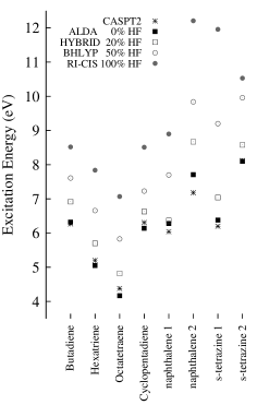
(b) Single excitations with D-CIS and D-TDDFT

The main interest of using a D-TDDFT kernel is to obtain the pure 2h2p states, which are not present in A-TDDFT and to better describe the 1h1p states of strong multireference character. We now take a closer look at the latter states in our test set. In particular, we will compare against the benchmarks those 1h1p states that have a 2h2p contribution larger than 10% (this percentage is determined by the CCSD calculation of Ref. SSS+08a .) The molecules containing such states are the four polyenes of the set, together with cyclopentadiene, naphthalene and s-triazine. From this sub-set, the polyenes are undoubtedly the ones which have been the most extensively discussed. Some debate persists as to whether A-TDDFT is able to represent a low-lying localized valence state which have a strong 2h2p contribution of the transition promoting two electrons from the highest- to the lowest-occupied molecular orbital. It was first shown by Hsu et al. that A-TDDFT with pure functionals gives the best answer for such states HHH01 , catching both the correct energetics and the localized nature of the state. Starcke et al. recognize this to be a fortuitous cancellation of errors SWS+06 .

In the top graph of Fig. 6 we show the the behavior of CIS (100% HF exchange) and A-TDDFT with different hybrids: ALDA with 0% HF exchange, ALDA with 20% HF exchange and BHLYP which has 50% HF exchange. In this comparison, we take the CASPT2 results (stars) as the benchmark result, since the best estimates were not provided for all the studied states SSS+08a . As seen in the graph, CIS (filled circles) seriously overestimate the excitation energies, consistent with the fact that it does not include any correlation effect. A-TDDFT with pure functionals give the best answer for doubly-excited states, very close to the CASPT2 result. This confirms the observation of Hsu et al. HHH01 Hybrid functionals, though giving the best overall answer, do not perform as good for these states. Additionally, the more HF exchange is mixed in the xc-kernel, the worse the result is. A different situation appears when we include explicitly 2h2p states. In Fig. 6 (b), we show the results of x-D-CIS and x-D-TDDFT. Now, the x-D-ALDA(10) underestimates the multireference excitation energies, due to overcounting of correlation effects. The best answer is now given by x-D-HYBRID(10) with 20% HF exchange. The x-D-CIS stays always higher. One can notice that the three last excitations (naphthalene 2 and s-triazine 1 and 2) are best described by the x-D-ALDA(10). This can be simply due to the fact that we missed the important double excitation to represent these states, since we restrict our calculation to 10 2h2p states and we add them in strict energetic order with no pre-screening.

VI Conclusion

D-TDDFT was introduced by Maitra et al. to explicitly include 2h2p states in TDDFT. The original work was ad hoc, leaving much room for variations on the original concept. A limited number of applications by Maitra and coworkers MZC+04 ; CZM+04 as well as by Mazur et al. MW09 ; MMR+10 showed promising results for D-TDDFT, but could hardly be considered definitive because (i) of the limited number of molecules and excitations treated and (ii) because the importance of the details of the specific implementations of D-TDDFT were not adequately explained. The present article has gone far towards remedying these problems, and providing further support for D-TDDFT.

We have implemented several variations of D-TDDFT and RI-CI in deMon2k, with the aim of characterizing the minimum necessary ingredients for an effective implementation of D-TDDFT. We have seen that DFT-based CIS gives very similar answers to HF-based CIS, showing that the effects of exact (HF) exchange can indeed be added in a post-SCF calculation. We have also found that although ALDA works better than CIS, it underestimates most of the excitation energies. Therefore, when we explicitly include 2h2p states through D-TDLDA, it leads to worse results, due to the double counting of correlation. The x-D-ALDA give least scatter of the results and hence a better answer. Nevertheless, the lower errors are still given by ALDA.

With the results of ALDA, we have shown that it is important to have a correct relative position of the 1h1p space and the 2h2p space in order to have a consistent account of correlation. We have introduced a hybrid TDDFT as a post-LDA calculation, and we have shown that the results are superior to those of ALDA. We have determined that the method giving the best answer for MR states is the combination of a hybrid xc-kernels with the 2h2p double excitations approximated with first-order corrections to the HF orbital energy differences.

Our work has gone much farther than previous work in testing D-TDDFT and in detailing the necessary ingredients to make it work well, We find a hybrid approach to be essential. We recognize that our work could be improved by a perturbative pre-selection procedure and consider this work to be ample justification for a more elaborate implementation of D-TDDFT. This work also constitutes a key step towards a full implementation of the polarization propatagor model of the exact $f_{xc}(\omega)$.

Appendix A Kohn-Sham-based Second-Order Polarization Propagator

In this appendix, we summarize the main expressions for the construction of the matrix elements of Eqs. (II) and (10). For a detailed derivation, the reader is referred to Ref. HC10 , in which this equations were derived for the construction of an exact ab initio xc-kernel consistent to second-order in perturbation theory.

The explicit expression for the single-single block is given by

$$[A_{11}]_{ai,bj}=$$

$$\left[\epsilon_{a}\delta_{ab}+(a|{\hat{M}}_{xc}|b)-\sum_{l}{\frac{(a|{\hat{M}}_{xc}|l)(l|{\hat{M}}_{xc}|b)}{\epsilon_{l}-\epsilon_{a}}}\right.$$

$$- \left.\frac{1}{2}\sum_{mld}{\frac{(ld||mb)(dl||ma)}{\epsilon_{m}+\epsilon_{l}-\epsilon_{d}-\epsilon_{a}}}\right]\delta_{ij}$$

$$- \left[\epsilon_{i}\delta_{ij}+(i|{\hat{M}}_{xc}|j)-\sum_{d}{\frac{(i|{\hat{M}}_{xc}|d)(d|{\hat{M}}_{xc}|j)}{\epsilon_{i}-\epsilon_{d}}}\right.$$

$$- \left.\frac{1}{2}\sum_{lke}{\frac{(le||jd)(dl||ei)}{\epsilon_{i}+\epsilon_{l}-\epsilon_{d}-\epsilon_{e}}}\right]\delta_{ab}\,,$$

the single-double block is given by

$$[A_{12}]_{ck,aibj} = \delta_{kj}(bc||ai)-\delta_{ki}(bc||aj)$$

$$+ \delta_{ac}(bi||kj)-\delta_{bc}(ai||kj)\,,$$

and the double-double block is given by

$$[A_{22}]_{aibj,ckdl}=\left(\epsilon_{b}+\epsilon_{a}-\epsilon_{i}-\epsilon_{j}\right)\delta_{ac}\delta_{ik}\delta_{bd}\delta_{jl}\,.$$ (15)

there $(pq||rs)=(pq|rs)-(qs|rq)$, where

$$(pq|rs)=\int{d^{3}rd^{3}r^{\prime}\psi^{*}_{p}({\bf r})\psi_{q}({\bf r})\frac{1}{|{\bf r}-{\bf r}^{\prime}|}\psi^{*}_{r}({\bf r}^{\prime})\psi^{*}_{s}({\bf r}^{\prime})}\,.$$ (16)

The first-order double-double block is given by

$$[A_{22}]_{aibj,ckdl}=$$

$$\left[\left(\epsilon_{b}\delta_{bd}+(b|{\hat{M}}_{xc}|d)\right)\delta_{ac}+\left(\epsilon_{a}\delta_{ac}+(a|{\hat{M}}_{xc}|c)\right)\delta_{bd}\right]\delta_{ik}\delta_{jl}$$

$$- \left[\left(\epsilon_{i}\delta_{ik}+(i|{\hat{M}}_{xc}|k)\right)\delta_{jl}-\left(\epsilon_{j}\delta_{jl}+(d|{\hat{M}}_{xc}|l)\right)\delta_{ik}\right]\delta_{ac}\delta_{bd}$$

$$- \delta_{ac}f(bd)-\delta_{bd}f(ac)+\delta_{ad}f(bc)+\delta_{bc}f(ad)$$

$$- \delta_{ac}\delta_{bd}(kj||li)-\delta_{jl}\delta_{ki}(ad||bc)\,,$$

with

$$f(pq) = \delta_{ik}(lj||pq)+\delta_{jl}(ki||pq)$$ (18)

$$- \delta_{kj}(li||pq)-\delta_{il}(kj||pq)\,.$$

Integrals with double bar are defined as in Eq. (I), in which the kernel $f$ is defined by $f({\bf r}_{1},{\bf r}_{2})=(1-{\hat{P}}_{12})/|{\bf r}_{1}-{\bf r}_{2}|$, where $P_{12}$ is the permutation operator that permutes the coordinates of two electrons.

Appendix B Tables of D-TDDFT and CISD excitation energies and oscillator strengths

Table 3: Singlet and Triplet excitation energies and oscillator strengths. All excitation energies are in eV. The CASPT2, Best Estimates (Best) and B3LYP calculations are taken from Refs. SSS+08a  and SSS+08b . The HF-based CIS calculations (CIS) are done with Gaussian03 g03 . The rest are done in deMon2k deMon2k .

Ethene	CASPT2	Best	B3LYP	CIS	RI-CIS	D-CIS	x-D-CIS	ALDA	DALDA	x-D-ALDA	hybrid	x-D-hybrid
$1^{1}B_{1u}$	7.98	7.8	7.7	8.15	7.94	7.94	7.94	9.44	9.44	9.44	9.24	9.24
f	0.36		0.362	0.633	0.59	0.59	0.59	0.507	0.507	0.507	0.558	0.558
$1^{3}B_{1u}$	4.39	4.5	4.03	3.46	3.26	3.26	3.26	5.95	5.95	5.95	5.54	5.55
Butadiene
$2^{1}A_{g}$	6.27	6.55	6.82	8.52	8.16	5.46	6.72	6.32	3.78	4.67	6.92	6.36
$1^{1}B_{u}$	6.23	6.18	5.74	6.55	6.43	5.52	6.23	6.64	4.98	6.12	6.81	6.67
f	0.686		0.672	1.214	1.31	0.885	1.22	0.922	0.47	0.726	1.07	1.02
$1^{3}A_{g}$	4.89	5.08	4.86	4.26	4.25	4.25	4.25	6.21	6.21	6.21	6.12	6.12
$1^{3}B_{u}$	3.2	3.2	2.76	2.48	2.12	1.94	2.06	4.08	3.31	3.81	3.9	3.83
Hexatriene
$2^{1}A_{g}$	5.2	5.09	5.69	7.84	7.55	4.06	5.68	5.05	2.23	3.43	5.7	5.05
$1^{1}B_{u}$	5.01	5.1	4.69	5.56	5.43	4.44	4.97	5.36	3.28	4.19	5.62	5.23
f	0.85		1.063	1.8031	2.16	1.25	1.83	1.55	0.362	0.856	1.86	1.61
$1^{3}A_{g}$	4.12	4.15	3.92	3.47	3.37	3.33	3.34	4.93	4.54	4.87	4.98	4.93
$1^{3}B_{u}$	2.55	2.4	2.09	1.95	1.49	1.3	1.37	3.13	2.21	2.59	3.04	2.86
Octatetraene
$2^{1}A_{g}$	4.38	4.47	4.84	7.07	6.79	3.17	4.95	4.17	1.57	2.76	4.82	4.23
$3^{1}A_{g}$	6.56	6.4	6.02	7.5	6.88	5.5	6.58	6.51	4.8	5.08	6.33	6.07
$4^{1}A_{g}$	7.14		6.35	7.77	7.69	6.03	7.06	7.05	7.23	6.43	6.96	6.92
$1^{1}B_{u}$	4.42	4.66	4.02	4.9	4.74	3.76	4.38	4.55	2.5	3.52	4.85	4.49
f	1.832		1.471	2.365	3.06	1.62	2.69	2.21	0.381	1.16	2.73	2.33
$2^{1}B_{u}$	5.83	5.76	6.78	8.13	7.69	4.4	6.19	6.21	5.82	5.85	6.08	5.31
f	0.01		0.029	0.055	0.031	0.041	0.0026	0.001	1.66	1.02	0.003	0
$3^{1}B_{u}$	8.44		7.41	8.69	8.33	7.83	8.18	8.04	7.93	7.93	7.05	6.76
f	0.002		0.145	0.055	0.082	0.129	0.319				0.124	0.362
$1^{3}A_{g}$	2.17	2.2	1.68	2.89	2.73	2.62	2.7	4.07	3.59	3.99	4.14	4.11
$1^{3}B_{u}$	3.39	3.55	3.24	1.63	1.09	0.92	1	2.56	1.62	2.08	2.52	2.36
Cyclopropene
$1^{1}B_{1}$	6.36	6.76	6.46	7.4	7.16	7.04	7.16	6.28	6.13	6.27	6.43	6.43
f	0.01		0.001	0.003	0.003	0.003	0.003	0.002	0.002	0.002	0.002	0.002
$1^{1}B_{2}$	7.45	7.06	6.31	7.01	6.81	6.81	6.81	6.77	6.77	6.77	7.03	7.03
f	0.101		0.074	0.184	0.167	0.167	0.167	0.051	0.052	0.052	0.082	0.082
$1^{3}B_{2}$	4.18	4.34	3.7	3.26	3.07	3.07	3.07	5.11	5.11	5.11	4.93	4.93
$1^{3}B_{1}$	6.05	6.62	6.01	6.89	6.68	6.61	6.68	5.91	5.82	5.91	6.06	6.06
Cyclopentadiene
$2^{1}A_{1}$	6.31	6.31	6.52	8.51	8.22	5.93	6.68	6.14	4.52	4.9	6.63	6.28
f	0		0.007	0.02	0.01	0.001	0.001	0.01	0	0	0.013	0.005
$3^{1}A_{1}$	7.89		8.15	9.08	8.8	8.8	8.49	9.03	8.11	8.6	9.32	9.21
f	0.442		0.563	1.077	0.981	0.956	0.814	0.488	0.118	0.332	0.754	0.764
$1^{1}B_{2}$	5.27	5.55	5.02	5.67	5.46	5.21	5.34	5.76	5.22	5.51	5.83	5.77
f	0.148		0.09	0.15	0.157	0.156	0.155	0.142	0.135	0.137	0.148	0.148
$1^{3}A_{1}$	4.9	5.09	4.75	4.26	4.26	4.26	4.26	5.86	5.86	5.86	5.89	5.89
$1^{3}B_{2}$	3.15	3.25	2.71	2.4	2.15	2.05	2.09	3.95	3.57	3.76	3.76	3.72
Norbornadiene
$1^{1}A_{2}$	5.28	5.34	4.79	5.8	5.54	5.54	5.54	4.75	4.75	4.75	5.19	5.19
$2^{1}A_{2}$	7.36		6.86	8.24	7.93	7.93	7.93	6.81	6.82	6.76	7.28	7.28
$1^{1}B_{2}$	6.2	6.11	5.52	7.29	7.01	7.01	7.01	5.09	5.09	5.09	5.64	5.64
f	0.008	0.029	0.01	0.16	0.124	0.124	0.124	0.006	0.006	0.006	0.009	0.009
$2^{1}B_{2}$	6.48		6.87	8.16	7.89	7.89	7.89	7.09	7.09	7.09	7.64	7.64
f	0.343	0.187	0.173	0.353	0.338	0.338	0.336	0.063	0.063	0.063	0.124	0.124
$1^{3}A_{2}$	3.42	3.72	3.08	2.81	2.65	2.65	2.65	4.11	4.11	4.11	4.15	4.15
$1^{3}B_{2}$	3.8	4.16	3.62	3.16	2.99	2.99	2.99	4.75	4.75	4.75	4.86	4.86

Benzene	CASPT2	Best	B3LYP	CIS	RI-CIS	D-CIS	x-D-CIS	ALDA	DALDA	x-D-ALDA	hybrid	x-D-hybrid
$1^{1}B_{1u}$	6.3	6.54	6.1	6.27	6.12	6.12	6.12	6.89	6.89	6.01	7.03	7.03
$1^{1}B_{2u}$	4.84	5.08	5.4	6.44	6.32	6.32	6.32	5.36	5.36	5.36	5.56	5.56
$11E_{1u}$	7.03	7.13	7.07	8.29	8.08	8.08	8.08	8.02	8.02	8.02	8.09	8.1
f	0.82		1.195	1.17	1.09	1.09	1.09	0.884	0.884	0.884	0.941	0.941
$11E_{2g}$	7.9	8.41	8.91	10.81	10.68	9.18	10.19	9.04	9.04	9.04	9.71	9.7
$1^{3}B_{1u}$	3.89	4.15	3.77	3.34	3.13	3.13	3.13	5.18	5.18	5.18	5.13	5.13
$1^{3}B_{2u}$	5.49	5.88	5.09	5.98	5.86	5.86	5.86	5.34	5.34	5.34	5.38	5.38
$13E_{1u}$	4.49	4.86	4.7	5.08	4.92	4.92	4.92	5.27	5.27	5.27	5.27	5.27
$13E_{2g}$	7.12	7.51	7.33	7.82	7.69	6.41	6.53	7.96	6.42	7.57	7.73	7.73
Naphthalene
$2^{1}A_{g}$	5.39	5.87	6.18	7.55	7.42	5.14	6.88	5.07	3.75	4.31	5.69	5.4
$3^{1}A_{g}$	6.04	6.67	6.85	9.13	8.9	6.49	7.17	6.28	6.71	5.82	6.37	6.12
$1^{1}B_{2u}$	4.56	4.77	4.35	5.26	5.06	5.06	5.06	4.47	4.47	4.47	4.83	4.83
f	0.05		0.062	0.114	0.112	0.112	0.122	0.056	0.056	0.056	0.081	0.081
$2^{1}B_{2u}$	5.93	6.33	6.12	7.45	7.22	7.22	7.22	6.49	6.49	6.49	6.83	6.83
f	0.313		0.186	0.684	0.601	0.601	0.601	0.158	0.158	0.158	0.24	0.24
$3^{1}B_{2u}$	7.16		7.87	9.85	9.67	9.66	9.67	8.29	8.29	8.29	8.62	8.62
f	0.848		0.532	0.806
$1^{1}B_{3u}$	4.03	4.24	4.44	5.38	5.16	5.16	5.16	4.3	4.3	4.31	4.56	4.56
f	0.001		0	0	0	0	0	0	0	0	0	0
$2^{1}B_{3u}$	5.54	6.06	5.93	7.23	7.12	7.12	7.11	6.46	6.46	6.46	6.71	6.72
f	1.337		1.268	2.483	2.5	2.5	2.49	1.74	1.74	1.74	2	2
$3^{1}B_{3u}$	7.18		8.65		12.21	11.14	9.52	7.71	7.71	7.14	8.67	8.63
f	0.048		0.01							0.033
$1^{1}B_{1g}$	5.53	5.99	5.58	6.95	6.78	5.68	6.62	5.95	5.47	6.26	6.37	6.12
$2^{1}B_{1g}$	5.87	6.47	6.32	8.08	7.85	6.65	6.96	7.03	6.71	6.98	7.06	6.44
$1^{3}A_{g}$	5.27	5.52	5.33	5.41	5.38	5.13	5.27	5.81	5.34	5.05	5.11	5.11
$2^{3}A_{g}$	5.83	6.47	5.95	7.21	6.95	5.93	6.28	5.92	5.87	5.69	5.67	5.5
$3^{3}A_{g}$	5.91	6.79	6.07	7.53	7.39	6.7	6.88	6.11	6.16	5.82	6.02	6
$1^{3}B_{2u}$	3.1	3.11	2.69	2.52	2.25	2.25	2.25	3.49	3.49	3.49	3.53	3.53
$2^{3}B_{2u}$	4.3	4.64	4.4	4.84	4.71	4.71	4.71	5.05	5.05	5.05	5.1	5.1
$1^{3}B_{3u}$	3.89	4.18	3.95	4.36	4.23	4.23	4.22	4.18	4.18	4.18	4.35	4.35
$2^{3}B_{3u}$	4.45	5.11	4.22	5.16	4.95	4.95	4.95	4.25	4.25	4.24	4.44	4.44
$1^{3}B_{1g}$	4.23	4.47	4.17	4.02	3.89	3.83	3.86	5.04	4.21	4.61	5.1	5.1
$2^{3}B_{1g}$	5.71	6.48	5.55	7.45	7.17	6.06	6.9	5.2	5.15	5.18	5.67	5.5
$3^{3}B_{1g}$	6.23	6.76	6.56	7.97	7.71	6.64	7.14	6.9	6.37	6.72	7.26	7.19
Furan
$2^{1}A_{1}$	6.16	6.57	6.7	8.25	8.02	5.12	6.97	6.54	3.35	5.37	6.92	6.53
f	0.002		0	0.001	0	0.007	0.028	0	0.001	0.004	0	0.001
$3^{1}A_{1}$	7.66	8.13	8.25	9.33	9.04	8.41	8.77	9.41	8.45	9.04	9.43	9.28
f	0.416		0.437	0.863	0.756	0.556	0.669	0.514	0.185	0.479	0.607	0.599
$1^{1}B_{2}$	6.04	6.32	6.16	6.69	6.35	6.12	6.17	7.06	6.51	6.62	7.09	7
f	0.154		0.162	0.216	0.214	0.202	0.213	0.277	0.227	0.238	0.279	0.276
$1^{3}A_{1}$	5.15	5.48	5.21	4.94	4.97	4.33	4.97	6.1	5.41	6.1	6.1	6.1
$1^{3}B_{2}$	3.99	4.17	3.71	3.26	2.99	2.84	2.94	4.92	4.39	4.72	4.74	4.69
Pyrrole
$2^{1}A_{1}$	5.92	6.37	6.53	7.79	7.61	6.93	6.96	6.46	6.39	5.54	6.78	6.58
f	0.02		0.001	0.006	0.002	0.009	0.009	0.001	0.001	0.002	0.002	0
$3^{1}A_{1}$	7.46	7.91	7.96	9.05	8.8	8.59	8.6	8.89	8.46	8.55	8.96	8.91
f	0.326		0.451	0.876	0.78	0.601	0.621	0.383	0.317	0.367	0.628	0.628
$1^{1}B_{2}$	6	6.57	6.4	6.94	6.7	6.57	6.37	7.27	6.62	6.65	7.27	7.15
f	0.125		0.173	0.236	0.232	0.189	0.198	0.265	0.177	0.183	0.28	0.268
$1^{3}A_{1}$	5.16	5.51	5.25	5.24	5.24	5.24	5.24	5.91	5.4	5.91	5.93	5.93
$1^{3}B_{2}$	4.27	4.48	4.07	3.69	3.51	3.44	3.4	5.18	4.73	4.75	5.02	4.91

Imidazole	CASPT2	Best	B3LYP	CIS	RI-CIS	D-CIS	x-D-CIS	ALDA	DALDA	x-D-ALDA	hybrid	x-D-hybrid
$2^{1}A^{\prime}$	6.72	6.19	6.45	7.23	6.97	6.89	6.45	6.72	5.38	5.64	6.97	6.67
f	0.126		0.144	0.26	0.254	0.23	0.211	0.072	0.05	0.061	0.093	0.096
$3^{1}A^{\prime}$	7.15	6.93	7.04	8.15	7.9	7.3	7.46	7.58	7.05	7.2	7.29	7.25
f	0.143		0.029	0.025	0.05	0.094	0.083	0.137	0.133	0.123	0.004	0.016
$4^{1}A^{\prime}$	8.51		8.27	9.43	9.22	9.03	9.85	7.96	7.93	7.96	7.46	7.43
f	0.594		0.359	0.65	0.471	0.328	0.156	0.026	0.014	0.013	0.209	0.192
$1^{1}A"$	6.52	6.81	6.46	7.63	7.5	7.39	7.43	5.56	5.5	5.52	6.14	6.14
f	0.011		0.003	0.014	0.015	0.015	0.015	0.001	0.001	0.001	0.002	0.002
$2^{1}A"$	7.56		7.45	9.58	9.35	8.47	8.53	7.31	6.92	7.03	6.37	6.36
f	0.013		0.005	0	0.001	0.001	0.001	0.02	0.018	0.019	0.001	0
$1^{3}A^{\prime}$	4.49	4.69	4.24	3.9	3.72	3.72	3.71	5.29	5.23	5.23	5.12	5.11
$2^{3}A^{\prime}$	5.47	5.79	5.44	5.38	5.32	5.32	5.29	6.3	6.23	6.3	6.19	6.18
$3^{3}A^{\prime}$	6.53	6.55	5.95	6.59	6.22	6.22	6.22	6.6	6.5	6.51	6.56	6.55
$4^{3}A^{\prime}$	7.08		6.93	7.92	7.58	7.58	7.52	7.64	7.64	7.64	7.54	7.54
$1^{3}A"$	6.07	6.37	5.83	6.39	6.3	6.22	6.24	5.33	5.3	5.31	5.78	5.78
$2^{3}A"$	7.15		6.86	7.72	8.72	7.83	7.78				6.59	6.51
Pyridine
$2^{1}A_{1}$	6.42	6.26	6.31	6.69	6.55	6.45	6.54	7.07	6.87	7.07	7.23	7.23
f	0.005		0.016	0.01	0.011	0.002	0.095	0.014	0.002	0.012	0.025	0.024
$3^{1}A_{1}$	7.23	7.18	7.32	8.59	8.37	7.46	8.35	8.32	8.37	8.31	8.43	8.43
f	0.82		0.424	1.049	0.956	0.138	0.955	0.604	0.543	0.643	0.774	0.775
$1^{1}B_{2}$	4.84	4.85	5.49	6.39	6.19	6.17	6.18	5.51	5.49	5.51	5.71	5.71
f	0.018		0.035	0.064	0.078	0.071	0.077	0.018	0.016	0.018	0.023	0.023
$2^{1}B_{2}$	7.48	7.27	7.3	8.58	8.4	7.75	8.39	8.05	7.39	8.05	8.13	8.13
f	0.64		0.455	0.95	0.843	0.151	0.843	0.654	0.002	0.659	0.515	0.517
$1^{1}B_{1}$	4.91	4.59	4.8	5.89	5.69	5.5	5.55	4.29	3.91	2.99	4.8	4.8
f	0.009		0.004	0.011	0.011	0.01	0.011	0.005	0.003	0.002	0.007	0
$1^{1}A_{2}$	5.17	5.11	5.11	7.38	7.23	7.22	7.23	4.12	4.11	4.11	4.77	4.39
$1^{3}A_{1}$	4.05	4.06	3.89	3.42	3.17	3.17	3.17	5.36	5.36	5.36	5.22	5.22
$2^{3}A_{1}$	4.73	4.91	4.84	5.18	5.01	5.01	5.01	5.6	5.6	5.6	5.49	5.49
$3^{3}A_{1}$	7.34		7.44	7.82	7.66	7.66	7.66	8.16	8.16	8.16	8.38	8.38
$1^{3}B_{2}$	4.56	4.64	4.51	5.01	4.76	4.76	4.76	4.93	4.93	4.93	5.01	5.01
$2^{3}B_{2}$	6.02	6.08	5.64	6.46	6.35	6.31	6.35	5.87	5.81	5.86	6	6
$3^{3}B_{2}$	7.28		7.75	8.33	8.23	7.78	8.23	8.5	8.5	8.5	8.7	8.7
$1^{3}B_{1}$	4.41	5.25	4.04	4.77	4.62	4.47	4.5	3.71	3.45	3	4.07	3.87
$1^{3}A_{2}$	5.1	5.28	4.98	7.17	7.02	7.01	7.02	4.02	4.01	4.02	4.69	4.69
Pyrazine
$1^{1}B_{1u}$	6.7	6.58	6.5	6.86	6.72	6.43	6.65	7.38	7.53	7.32	7.48	7.48
f	0.08		0.059	0.039	0.042	0.001	0.025	0.071	0.157	0.037	0.101	0.096
$2^{1}B_{1u}$	7.57	7.72	7.68	8.9	8.68	7.36	8.4	8.31	8.39	8.27	8.64	8.62
f	0.76		0.367	0.903	0.795	0.193	0.705	0.039	0	0.05	0.375	0.388
$1^{1}B_{2u}$	4.75	4.64	5.37	6.25	5.93	5.91	5.92	5.52	5.48	5.51	5.71	5.7
f	0.07		0.091	0.171	0.182	0.127	0.18	0.062	0.054	0.059	0.077	0.076
$2^{1}B_{2u}$	7.7	7.6	7.78	9.13	9.07	7.84	9	8.47	8.7	8.42	8.67	8.66
f	0.66		0.264	0.73	0.597	0.108	0.589	0.689	0.69	0.691	0.819	0.819
$1^{1}A_{u}$	4.52	4.81	4.69	6.84	6.61	6.61	6.61	3.62	3.62	3.62	4.27	4.27
$1^{1}B_{1g}$	6.13	6.6	6.38	9.75	9.62	9.62	9.62	5.17	5.17	5.17	6.05	6.05
$1^{1}B_{2g}$	5.17	5.56	5.55	6.53	6.34	6.34	6.34	5.04	5.04	5.04	5.66	5.66
$1^{1}B_{3u}$	3.63	3.95	3.96	4.9	4.63	4.63	4.63	3.44	3.44	3.44	3.88	3.88
f	0.01		0.006	0.016	0.016	0.016	0.0157	0.007	0.007	0.007	0.009	0.009
Pyrimidine
$2^{1}A_{1}$	6.72	6.95	6.58	7.04	6.87	6.9	6.84	7.32	7.26	7.3	7.52	7.51
f	0.05		0.037	0.021	0.025	0.04	0.023	0.059	0.037	0.051	0.074	0.07
$3^{1}A_{1}$	7.57		7.48	8.75	8.55	8.62	8.53	8.4	7.75	8.36	8.34	8.32
f	0.58		0.386	0.863	0.778	0.72	0.777	0.498	0.055	0.5	0.317	0.325
$1^{1}B_{2}$	4.93	5.44	5.74	6.69	6.48	6.43	6.49	5.74	5.7	5.73	5.95	5.95
f	0.001		0.034	0.068	0.081	0.077	0.081	0.018	0.018	0.018	0.023	0.023
$2^{1}B_{2}$	7.32		7.76	8.99	8.84	8.89	8.82	8.58	8.62	8.57	7.6	7.6
f	0.79		0.297	0.852	0.764	0.745	0.759	0.411	0.483	0.365	0.007	0.007
$1^{1}B_{1}$	3.81	4.55	4.27	5.64	5.41	5.41	5.41	3.59	3.59	3.59	4.14	4.14
f	0.02		0.005	0.018	0.019	0.019	0.019	0.005	0.005	0.005	0.008	0.075
$1^{1}A_{2}$	4.12	4.91	4.6	6.31	6.13	6.13	6.13	3.68	3.68	3.68	4.33	4.33

Pyridazine	CASPT2	Best	B3LYP	CIS	RI-CIS	D-CIS	x-D-CIS	ALDA	DALDA	x-D-ALDA	hybrid	x-D-hybrid
$2^{1}A_{1}$	4.86	5.18	5.61	6.52	6.32	6.42	6.3	5.62	4.48	5.6	5.83	5.82
f	0.009		0.022	0.044	0.051	0.045	0.053	0.009	0.003	0.01	0.013	0.013
$3^{1}A_{1}$	7.5		7.5	8.8	8.6	7.3	8.59	8.45	8.48	8.42	8.13	8.13
f	0.5		0.335	0.873	0.766	0.062	0.706	0.489	0.412	0.513	0.572	0.572
$1^{1}B_{2}$	6.61		6.43	6.76	6.62	6.35	6.57	7.11	7.2	7.09	6.75	6.75
f	0.003		0.002	0.002	0.004	0.002	0.005	0.002	0	0.0039	0.002	0.002
$2^{1}B_{2}$	7.39		7.24	8.47	8.22	8.3	8.2	8.07	8.1	8.04	7.36	7.35
f	0.75		0.431	0.855	0.756	0.72	0.75	0.535	0.506	0.539	0.001	0.002
$1^{1}A_{2}$	3.66	4.31	4.18	5.83	5.65	5.65	5.6	3.16	3.16	3.16	3.87	3.87
$2^{1}A_{2}$	5.09	5.77	5.44	7.18	6.84	6.84	6.68	4.87	4.87	4.87	5.35	5.35
$1^{1}B_{1}$	3.48	3.78	3.58	4.71	4.45	4.45	4.22	2.99	2.99	2.44	3.5	3.34
f	0.01		0.005	0.017	0.017	0.017	0.015	0.005	0.005	0.003	0.007	0.007
$2^{1}B_{1}$	5.8		6.09	8.3	8.12	8.12	8.01	5.1	5.1	5.06	5.82	5.82
f	0.008		0.005	0.007	0.008	0.008	0.001	0.005	0.005	0.003	0.013	0.013
s-triazine
$2^{1}A^{\prime}$	6.77		7.01	7.52	7.31	6.88	7.3	7.84	7.92	7.82	7.24	7.24
$1^{1}A_{2}^{\prime}$	5.53	5.79	6.14	7.2	7.08	6.79	7.08	6.02	5.96	6.01	6.25	6.25
$11E^{\prime}$	8.16		7.79	9.1	8.93	8.96	8.91	8.49	8.53	8.48	8.66	8.65
f	0.61		0.762	0.768	0.717	0.704	0.716	0.258	0.246		0.463	0.468
$1^{1}A_{1}"$	3.9	4.6	4.45	6.6	6.51	6.51	6.51	3.39	3.39	3.39	4.09	4.06
$1^{1}A_{2}"$	4.08	4.66	4.54	5.93	5.68	5.68	5.68	3.9	3.9	3.9	4.41	4.41
f	0.015		0.014	0.039	0.042	0.042	0.042	0.018	0.018		0.024	0.024
$11E"$	4.36	4.7	4.54	6.16	5.98	5.98	5.98	3.64	3.64	3.64	4.26	4.26
$21E"$	7.15		7.49	9.44	9.32	9.32	9.32	7.64	7.64	7.64	7.26	7.26
s-tetrazine
$1^{1}A_{u}$	3.06	3.51	3.51	5.27	5.02	4.22	5.02	2.38	2.38	2.38	3.17	3.17
$2^{1}A_{u}$	5.28	5.5	5.04	6.44	6.03	6.35	6.03	4.22	4.22	4.22	4.81	4.81
$1^{1}B_{1g}$	4.51	4.73	4.73	5.93	5.71	5.71	5.71	3.76	3.76	3.76	4.67	4.67
$2^{1}B_{1g}$	5.99		6.64	9.76	9.47	9.47	9.47	5.35	5.35	5.35	6.49	6.49
$3^{1}B_{1g}$	6.2		7.4	11.96	11.48	11.23	11.48	6.38	6.38	6.38	7.04	7.04
$1^{1}B_{2g}$	5.05	5.2	5.29	6.44	6.11	6.11	6.11	4.39	4.39	4.39	5.21	5.21
$2^{1}B_{2g}$	5.48		5.99	9.32	9.06	9.06	9.06	5.04	5.04	5.04	5.84	5.84
$2^{1}B_{3g}$	8.12		9.3	10.53	10.77	10.05	10.77	8.1	8.1	8.1	8.58	8.58
$1^{1}B_{1u}$	7.13		6.9	7.08	6.92	7.04	6.85	7.81	7.84	7.71	8.05	8.04
f	0.001		0.002	0	0	0.002	0	0.033	0.059	0.023	0.004	0.004
$2^{1}B_{1u}$	7.54		7.48	8.7	8.43	8.48	8.43	8.24	8.32	8.23	8.42	8.42
f	0.687		0.337	0.645	0.559	0.546	0.559	0.345	0.307	0.355	0.436	0.436
$1^{1}B_{2u}$	4.89	4.93	5.58	6.51	6.22	6.35	6.11	5.71	5.82	5.64	5.92	5.91
f	0.045		0.064	0.133	0.14	0.126	0.139	0.039	0.032	0.042	0.054	0.055
$2^{1}B_{2u}$	7.94		8.26	9.53	9.42	9.43	9.46	9	9.02	9.13	9.19	9.19
f	0.733		0.29	0.562	0.462	0.464	0.459	0.361			0.445	0.444
$1^{1}B_{3u}$	1.96	2.29	2.24	3.33	2.94	2.94	2.94	1.62	1.62	1.62	2.11	2.11
f	0.013		0.005	0.022	0.021	0.021	0.021	0.006	0.006	0.006	0.01	0.01
$2^{1}B_{3u}$	6.37		6.29	8.34	8.14	8.14	8.14	5.08	5.08	5.08	5.93	5.93
f	0.017		0.01	0.023	0.026	0.026	0.026	0.011	0.011	0.011	0.016	0.016
$1^{3}A_{u}$	2.81	3.52	3.1	4.23	4.04	4.02	4.04	2.15	2.15	2.15	2.86	2.86
$2^{3}A_{u}$	4.85	5.03	4.43	6.07	5.64	4.36	5.64	3.69	3.69	3.69	4.23	4.23
$1^{3}B_{1g}$	3.76	4.21	3.63	4.13	3.98	3.98	3.98	3.16	3.16	3.16	3.69	3.69
$2^{3}B_{1g}$	5.68		6.33	9.67	9.37	9.37	9.37	5.32	5.32	5.32	6.13	6.13
$1^{3}B_{1u}$	4.25	4.33	3.83	3.04	2.74	2.74	2.74	5.7	5.7	5.66	5.44	5.44
$2^{3}B_{1u}$	5.09	5.38	5.24	5.69	5.55	5.56	5.5	5.96	5.96	5.94	5.94	5.93
$1^{3}B_{2g}$	4.67	4.93	4.48	5.13	4.91	4.91	4.91	4.17	4.17	4.17	4.61	4.61
$2^{3}B_{2g}$	5.3		5.62	8.96	8.66	8.66	8.66	4.33	4.33	4.33	5.33	5.33
$1^{3}B_{2u}$	4.29	4.54	4.06	4.41	4.02	4.02	4.02	4.68	4.68	4.68	4.67	4.67
$2^{3}B_{2u}$	6.81		6.63	7.59	7.6	7.6	7.6	6.8	6.8	6.8	7.02	7.02
$1^{3}B_{3u}$	1.45	1.89	1.42	2.07	1.74	1.74	1.74	0.99	0.99	0.99	1.36	1.36
$2^{3}B_{3u}$	6.14		5.97	7.9	7.7	7.7	7.7	4.85	4.85	4.85	5.64	5.64

Formaldehyde	CASPT2	Best	B3LYP	CIS	RI-CIS	D-CIS	x-D-CIS	ALDA	DALDA	x-D-ALDA	hybrid	x-D-hybrid
$1^{1}A_{2}$	3.91	3.88	3.89	4.18	4.18	2.84	3.12	3.87	2.34	2.63	3.97	3.59
$1^{1}B_{1}$	9.09	9.1	8.89	9.19	9.21	9.2	9.2	9.02	9.01	9.02	9.06	9.06
f	0.01		0.001	0.002	0.001	0.001	0.001	0.003	0.003	0.003	0.003	0.003
$2^{1}A_{1}$	10.08	9.3	9.17	9.7	9.62	9.71	9.42	11.67	11.4	9.66	11.63	11.62
f	0.28		0.35	0.259	0.206	0.203	0.175	0.241	0.209	0.03	0.404	0.403
$1^{3}A_{2}$	3.48	3.5	3.13	3.4	3.4	2.65	2.82	3.23	2.34	2.52	3.33	3.1
$1^{3}A_{1}$	5.99	5.87	5.18	4.27	4.08	4.08	4.08	7.55	7.55	7.55	6.96	6.96
Acetone
$1^{1}A_{2}$	4.18	4.4	4.34	4.88	4.77	3.69	4.1	4.28	3.15	3.53	4.38	4.1
$1^{1}B_{1}$	9.1	9.17	8.6	9.4	9.35	9.36	9.29	7.83	7.82	7.83	8.49	8.49
f	0.01		0	0	0	0	0	0.004	0.004	0.004	0.002	0.002
$2^{1}A_{1}$	9.16	9.65	9.04	9.67	9.62	9.73	9.53	9.02	9.02	9.02	9.75	9.74
f	0.326		0.195	0.371	0.316	0.292	0.309	0.137	0.084	0.136	0.209	0.21
$1^{3}A_{2}$	3.9	4.05	3.69	4.17	4.07	3.49	3.71	3.74	3.13	3.32	3.83	3.66
$1^{3}A_{1}$	5.98	6.03	5.39	4.8	4.62	4.62	4.62	6.86	6.86	6.86	6.73	6.73
o-benzoquinone
$1^{1}A_{u}$	2.5	2.77	2.58	3.92	3.58	1.12	2.63	2.05	-0.74	0.58	2.62	2.04
$1^{1}B_{1g}$	2.5	2.76	2.43	3.73	3.32	3.32	3.32	1.83	1.83	1.83	2.33	2.33
$1^{1}B_{1u}$	5.15	5.28	4.83	6.23	6.13	6.18	6.01	4.93	4.98	4.91	5.37	5.37
f	0.616		0.323	1.154	1.23	1.2	1.14	0.242	0.225	0.284	0.36	0.362
$2^{1}B_{1u}$	7.08		7.25	8.89	8.5	8.5	8.5	7.38	7.4	7.2	8.09	8.08
f	0.624		0.561	0.721	0.724	0.725	0.73	0.231	0.225	0.192	0.487	0.487
$1^{1}B_{3g}$	4.19	4.26	3.73	5.21	4.51	4.51	4.51	3.31	3.31	3.31	3.77	3.77
f	0		0	0	0	0	0	0	0	0	0	0
$2^{1}B_{3g}$	6.34	6.96	6.59	8.58	8.46	8.46	8.46	6.46	6.54	6.54	7.06	7.06
$1^{1}B_{3u}$	5.15	5.64	5.43	8.27	7.96	7.97	7.97	4.41	4.41	4.41	5.41	5.41
f	0		0	0.016	0.014	0.014	0.014	0	0	0	0	0
$1^{3}A_{u}$	2.27	2.62	2.05	3.22	2.88	1.22	2.29	1.73	-0.51	0.6	2.18	1.91
$1^{3}B_{1g}$	2.17	2.51	1.92	3.05	2.67	2.67	2.67	1.48	1.48	1.48	1.91	1.78
$1^{3}B_{1u}$	2.91	2.96	2.19	2.04	1.42	1.42	1.42	3.15	3.13	3.15	3.09	3.09
$1^{3}B_{3g}$	3.19	3.41	2.68	2.72	2.36	2.36	2.35	2.89	2.89	2.89	3.13	3.13
Formamide
$2^{1}A^{\prime}$	7.41	7.39	8.13	8.73	8.67	7.47	7.93	8.82	8.92	7.98	8.78	8.76
f	0.371		0.371	0.278	0.206	0.078	0.032	0.383	0.036	0.346	0.123	0.179
$3^{1}A^{\prime}$	10.5		10.92	10.55	10.63	9.08	9.52	12.05	10.29	10.4	9.17	8.86
f	0.131		0.055	0.193	0.343	0.394	0.102	0.055	0.081	0.079	0.542	0.453
$1A"$	5.61	5.63	5.55	6.13	6.13	4.92	5.27	5.56	4.21	4.57	5.72	5.4
f	0.001		0.001	0.002	0.003	0.001	0.002	0.002	0	0.001	0.002	0.002
$1^{3}A^{\prime}$	5.69	5.74	5.13	5.14	4.86	4.85	4.86	5.93	5.93	4.63	5.92	5.92
$1^{3}A"$	5.34	5.36	4.97	5.51	5.47	4.69	4.93	5.06	4.21	4.42	5.21	4.99
Acetamide
$2^{1}A^{\prime}$	7.21	7.27	7.46	8.9	8.95	8.95	9.02	8.1	8.89	7.07	7.9	7.77
f	0.292		0.087	0.248	0.206	0.296	0.324	0.161	0.166	0.131	0.062	0.122
$3^{1}A^{\prime}$	10.08		10.01	11.51	11.2	10.25	9.91	9.65	9.52	9.14	8.45	8.28
f	0.179		0.224	0.114	0.162	0.034	0.202	0.173	0.05	0.142	0.156	0.09
$1^{1}A"$	5.54	5.69	5.56	6.36	6.3	5.31	5.54	5.51	4.46	4.63	5.65	5.38
f	0.001		0.001	0.001	0.001	0.001	0.001	0.002	0.001	0.001	0.003	0.002
$1^{3}A^{\prime}$	5.57	5.88	5.26	5.41	5.16	5.16	5.16	5.91	5.91	4.6	5.95	5.95
$1^{3}A"$	5.24	5.42	5.01	5.73	5.65	5.08	5.2	5.03	4.38	4.48	5.17	4.99
Propanamide
$2^{1}A^{\prime}$	7.28	7.2	7.76	8.92	8.92	7.42	8.32	7.77	7.77	7.77	6.95	6.29
f	0.346		0.107	0.287	0.206	0.121	0.038	0.067	0.067	0.068	0.012	0.011
$3^{1}A^{\prime}$	9.95		9	10.06	9.79	9.08	9.01	8.11	7.99	7.86	8.01	7.79
f	0.205		0.085	0.091	0.106	0.216	0.278	0.121	0.072	0.084	0.085	0.154
$1^{1}A"$	5.48	5.72	5.59	6.34	6.31	5.41	5.63	5.52	4.56	4.76	5.7	5.46
f	0.001		0	0.001	0.001	0.001	0.001	0.001	0.001	0.001	0.001	0.001
$1^{3}A^{\prime}$	5.94	5.9	5.28	5.46	5.22	5.22	5.22	5.89	5.89	5.89	5.97	5.97
$1^{3}A"$	5.28	5.45	5.04	5.76	5.67	5.16	5.27	5.05	4.45	4.58	5.21	5.06

Cytosine	CASPT2	Best	B3LYP	CIS	RI-CIS	D-CIS	x-D-CIS	ALDA	DALDA	x-D-ALDA	hybrid	x-D-hybrid
$2^{1}A^{\prime}$	4.39	4.66	4.64	6.09	5.94	5.18	5.64	4.51	3.47	3.78	4.99	4.33
f	0.061		0.035	0.161	0.182	0.069	0.105	0.022	0.014	0.005	0.046	0.014
$3^{1}A^{\prime}$	5.36	5.62	5.42	7.42	7.28	6.38	7.03	5.11	4.9	4.91	5.73	5.55
f	0.108		0.087	0.361	0.12	0.19	0.264	0.042	0.051	0.02	0.069	0.049
$4^{1}A^{\prime}$	6.16		6.72	7.91	7.83	7.03	7.79	6.17	5.98	5.89	6.76	6.41
f	0.863		0.368	0.819	1.03	0.176	0.934	0.115	0.019	0.124	0.136	0.196
$5^{1}A^{\prime}$	6.74		6.46	8.98	8.75	7.76	8.43	6.98	6.9	6.04	7.25	7.02
f	0.147		0.177	0.186	0.364	0.416	0.233	0.539	0.43	0.074	0.505	0.415
$1^{1}A"$	5	4.87	4.76	6.6	6.44	5.27	6.44	3.82	3.73	3.78	4.68	4.62
f	0.005		0.001	0.003	0.003	0.002	0.04	0	0	0	0.001	0.009
$2^{1}A"$	6.53	5.26	5.11	6.91	6.93	6.76	6.93	4.27	3.05	4.23	4.5	5.10
f	0.001		0.001	0.001	0.001	0	0.001	0.002	0.001	0.001	0	0.001
Thymine
$2^{1}A^{\prime}$	4.88	5.2	5	6.36	6.1	5.92	6.02	4.79	4.1	4.61	5.35	5.16
f	0.17		0.136	0.497	0.463	0.456	0.429	0.064	0.017	0.055	0.128	0.088
$3^{1}A^{\prime}$	5.88	6.27	5.97	8.16	7.8	6.12	7.3	5.62	4.56	5.81	6.31	5.88
f	0.17		0.071	0.202	0.29	0.018	0.288	0.099	0.069	0.073	0.14	0.117
$4^{1}A^{\prime}$	6.1	6.53	6.31	8.55	8.47	7.41	8.33	6.05	5.54	6.4	6.66	6.38
f	0.15		0.142	0.446	0.271	0.017	0.243	0.085	0.038	0.023	0.139	0.068
$5^{1}A^{\prime}$	7.16		7.47	9.48	9.44	7.88	9.21	7.13	6.77	7.16	7.92	7.39
f	0.85		0.411	0.182	0.173	0.198	0.408	0.11	0.059	0.092	0.542	0.189
$1^{1}A"$	4.39	4.82	4.7	6.01	5.96	4.97	5.96	4.21	2.98	3.66	4.81	4.24
$2^{1}A"$	5.91	6.16	5.8	7.41	7.12	7.12	7.05	4.83	4.45	4.69	5.89	5.83
$3^{1}A"$	6.15		6.21	7.65	7.43	7.37	7.43	5.21	5.21	5.19	6.18	6.09
$4^{1}A"$	6.7		6.69	8.83	8.24	8.18	8.24	6.13	6.06	5.21	6.7	6.66
f	0		0	0	0	0	0	0	0	0	0	0
Uracil
$2^{1}A^{\prime}$	5	5.35	5.19	6.55	6.31	5.82	6.31	4.95	4.5	4.95	5.52	5.51
f	0.19		0.13	0.51	0.475	0.323	0.475	0.044	0.011	0.044	0.105	0.105
$3^{1}A^{\prime}$	5.82	6.26	5.87	8.29	8	6.5	8	5.51	5.32	5.51	6.2	6.19
f	0.08		0.04	0.154	0.219	0.096	0.217	0	0.073	0.047	0.066	0.067
$4^{1}A^{\prime}$	6.46	6.7	6.5	8.66	8.51	7.63	8.51	6.43	6.19	6.18	6.84	6.83
f	0.29		0.12	0.43	0.344	0.011	0.345	0.112	0.035	0.036	0.145	0.151
$5^{1}A^{\prime}$	7		7.45	9.35	9.33	8.1	9.32	7.45	6.41	6.43	7.32	7.42
f	0.76		0.44	0.266	0.425	0.267	0.423	0.237	0.078	0.111	0.028	0.032
$1^{1}A"$	4.54	4.8	4.63	6	5.95	4.57	5.62	4.09	2.28	3.46	4.74	4.09
$2^{1}A"$	6	6.1	5.74	7.35	7.33	7.32	7.33	4.79	4.35	4.66	5.64	5.78
f	0		0	0	0.001	0	0.001	0	0	0	0	0
$3^{1}A"$	6.37	6.56	6.14	7.84	7.37	7.34	7.37	5.12	5.11	5.12	6.11	5.99
$4^{1}A"$	6.95		6.64	9.01	8.47	7.77	8.47	6.09	6.05	6.1	6.65	6.63
f	0		0	0.019	0.017	0	0.017	0	0	0	0	0
Adenine
$2^{1}A^{\prime}$	5.13	5.25	5.27	6.32	6.04	5.66	5.86	4.7	3.69	4.06	5.27	4.71
f	0.07		0.047	0.418	0.459	0.062	0.377	0.083	0.034	0.059	0.11	0.080
$3^{1}A^{\prime}$	5.2	5.25	5	6.51	6.27	6.08	6.13	5.21	5	4.9	5.6	5.41
f	0.37		0.195	0.041	0.025	0.367	0.097	0.072	0.013	0.016	0.182	0.001
$4^{1}A^{\prime}$	6.24		6.32	7.81	7.55	6.54	7.33	5.69	5.33	5.46	6.36	5.95
f	0.851		0.24	0.353	0.182	0.054	0.05	0.077	0.049	0.143	0.032	0.117
$5^{1}A^{\prime}$	6.72		6.69	8.28	8.04	6.94	7.85	5.96	5.47	5.72	6.63	6.46
f	0.159		0.107	0.48	0.704	0.023	0.744	0.065	0.126	0.0001	0.201	0.011
$6^{1}A^{\prime}$	6.99		7.08	8.45	8.29	7.7	8.13	6.46	6.05	6.07	7.15	6.68
f	0.565		0.137	0.571	0.492	0.589	0.324	0.034	0.002	0.09	0.218	0.264
$7^{1}A^{\prime}$	7.57		7.52	9.08	8.84	8.00	8.61	6.68	6.08	6.08	7.58	7.34
f	0.406		0.244	0.26	0.208	0.060	0.325	0.055	0.023	0.026	0.127	0.127
$1^{1}A"$	6.15	5.12	4.97	6.84	6.64	6.27	6.64	3.95	3.61	3.95	4.7	4.71
f	0.001		0	0	0.001	0.006	0.001	0	0	0	0	0.008
$2^{1}A"$	6.86	5.75	5.61	7.25	7.01	6.85	7.01	4.78	4.4	4.72	5.42	5.41
f	0.001		0.001	0.002	0.003	0.003	0.003	0	0.001	0	0.001	0.001

References

- (1) E. Runge and E. K. U. Gross, Density-Functional Theory for Time-Dependent Systems, Phys. Rev. Lett. 52, 997 (1984).
- (2) M. E. Casida, Propagator corrections to adiabatic time-dependent density-functional theory linear response theory., J. Chem. Phys. 122, 54111 (2005).
- (3) J. H. Starcke, M. Wormit, J. Schirmer, and A. Dreuw, How much double excitation character do the lowest excited states of linear polyenes have?, Chem. Phys. 329, 39 (2006).
- (4) B. O. Roos, Theoretical Studies of Electronically Excited States of Molecular Systems Using Multiconfigurational Perturbation Theory, Acc. Chem. Res. 32, 137 (1999).
- (5) B. G. Levine, C. Ko, J. Quenneville, and T. J. Martínez, Conical intersections and double excitations in time-dependent density functional theory, Mol. Phys. 104, 1039 (2006).
- (6) N. T. Maitra, F. Zhang, R. J. Cave, and K. Burke, Double excitations within time-dependent density functional theory linear response theory, J. Chem. Phys. 120, 5932 (2004).
- (7) R. J. Cave, F. Zhang, N. T. Maitra, and K. Burke, A dressed TDDFT treatment of the states of butadiene and hexatriene, Chem. Phys. Lett. 389, 39 (2004).
- (8) G. Mazur and R. Włodarczyk, Application of the dressed time-dependent density functional theory for the excited states of linear polyenes, J. Comput. Chem. 30, 811 (2009).
- (9) G. Mazur, M. Marcin, W. Rodoslaw, and Y. Aoki, Dressed TDDFT Study of Low-Lying Electronic Excited States in Selected Linear Polyenes and Diphenylopolyenes, Int. J. Quant. Chem. (2010), in press. DOI: 10.1002/qua.22876.
- (10) M. Schreiber, M. R. Silva-Junior, S. P. A. Sauer, and W. Thiel, Benchmarks for electronically excited states: CASPT2, CC2, CCSD, and CC3, J. Chem. Phys. 128, 134110 (2008).
- (11) M. R. Silva-Junior, M. Schreiber, S. P. A. Sauer, and W. Thiel, Benchmarks for electronically excited states: Time-dependent density functional theory and density functional theory based multireference configuration interaction, J. Chem. Phys. 129, 104103 (2008).
- (12) deMon2k@Grenoble, the Grenoble development version of deMon2k, Andreas M. Köster, Patrizia Calaminici, Mark E. Casida, Roberto Flores-Morino, Gerald Geudtner, Annick Goursot, Thomas Heine, Andrei Ipatov, Florian Janetzko, Sergei Patchkovskii, J. Ulisis Reveles, Dennis R. Salahub, and Alberto Vela, The International deMon Developers Community (Cinvestav-IPN, Mexico, 2006).
- (13) A. Zangwill and P. Soven, Density-functional approach to local-field effects in finite systems: Photoabsorption in the rare gases, Phys. Rev. A 21, 1561 (1980).
- (14) R. van Leeuwen, Causality and Symmetry in Time-Dependent Density-Functional Theory, Phys. Rev. Lett. 80, 1280 (1998).
- (15) A. K. Rajagopal, Time-dependent variational principle and the effective action in density-functional theory and Berry’s phase, Phys. Rev. A 54, 3916 (1996).
- (16) S. Mukamel, Generalized time-dependent density-functional-theory response functions for spontaneous density fluctuations and nonlinear response: Resolving the causality paradox in real time, Phys. Rev. A 71, 1 (2005).
- (17) G. Vignale, Real-time resolution of the causality paradox of time-dependent density-functional theory, Phys. Rev. A 77, 1 (2008).
- (18) T. A. Niehaus and N. H. March, Brief review related to the foundations of time-dependent density functional theory, Theor. Chem. Acc. 125, 427 (2009).
- (19) M. E. Casida, Time-dependent density-functional response theory for molecules, in Recent Advances in Density Functional Methods, Part I, edited by D. P. Chong, page 155, World Scientific, Singapore, 1995.
- (20) D. Bohm and D. Pines, A Collective Description of Electron Interactions: III. Coulomb Interactions in a Degenerate Electron Gas, Phys. Rev. 92, 609 (1953).
- (21) S. Hirata and M. Head-Gordon, Time-dependent density functional theory within the Tamm–Dancoff approximation, Chem. Phys. Lett. 314, 291 (1999).
- (22) M. E. Casida et al., Charge-transfer correction for improved time-dependent local density approximation excited-state potential energy curves: Analysis within the two-level model with illustration for H[sub 2] and LiH, J. Chem. Phys. 70, 933 (2000).
- (23) F. Cordova et al., Troubleshooting time-dependent density-functional theory for photochemical applications: oxirane., J. Chem. Phys. 127, 164111 (2007).
- (24) M. E. Casida, A. Ipatov, and F. Cordova, Linear-Response Time-Dependent Density-Functional Theory for Open-Shell Molecules, in Lecture Notes in Physics, edited by M. A. L. Marques, C. A. Ullrich, F. Nogueira, and A. Rubio, Springer, Berlin, 2006.
- (25) Z. Li and W. Liu, Spin-adapted open-shell random phase approximation and time-dependent density functional theory. I. Theory., J. Chem. Phys. 133, 064106 (2010).
- (26) M. Wanko et al., Calculating absorption shifts for retinal proteins: computational challenges., J. Phys. Chem. B 109, 3606 (2005).
- (27) C. Angeli, An analysis of the dynamic polarization in the V state of ethene, Int. J. Quant. Chem. 110, 2436 (2010).
- (28) R. J. Cave and E. R. Davidson, Theoretical Investigation of Several Low-Lying States of trans,trans-1,3,5-Hexatriene, J. Phys. Chem. 92, 614 (1988).
- (29) L. Serrano-Andrés, J. Sánchez-Marín, and I. Nebot-Gil, Theoretical study of the low-lying states of trans-1,3-butadiene, J. Chem. Phys. 97, 7499 (1992).
- (30) J. Lappe and R. J. Cave, On the Vertical and Adiabatic Excitation Energies of the 2 1 A g State of trans -1,3-Butadiene, J. Phys. Chem. A 104, 2294 (2000).
- (31) M. Boggio-Pasqua, M. J. Bearpark, M. Klene, and M. A. Robb, A computational strategy for geometry optimization of ionic and covalent excited states, applied to butadiene and hexatriene., J. Chem. Phys. 120, 7849 (2004).
- (32) J. Catalán and J. L. G. de Paz, On the photophysics of all-trans polyenes: hexatriene versus octatetraene., J. Chem. Phys. 124, 034306 (2006).
- (33) I. Mikhailov, S. Tafur, and A. Masunov, Double excitations and state-to-state transition dipoles in pi-pi* excited singlet states of linear polyenes: Time-dependent density-functional theory versus multiconfigurational methods, Phys. Rev. A 77, 012510 (2008).
- (34) G. Wald, The Molecular Basis of Visual Excitation, in Nobel Lectures, Physiology or Medicine 1963-1970, pages 293–315, Elsevier Publishing Company, Amsterdam, 1972.
- (35) R. Granit, The Development of Retinal Neurophysiology., in Nobel Lectures, Physiology or Medicine 1963-1970, pages 255–265, Elsevier Publishing Company, Amsterdam, 1972.
- (36) H. K. Hartline, Visual Receptors and Retinal Interaction., in Nobel Lectures, Physiology or Medicine 1963-1970, pages 269–288, Elsevier Publishing Company, Amsterdam, 1972.
- (37) A. I. Krylov, Spin-flip configuration interaction: an electronic structure model that is both variational and size-consistent, Chem. Phys. Lett. 350, 522 (2001).
- (38) F. Wang and T. Ziegler, Time-dependent density functional theory based on a noncollinear formulation of the exchange-correlation potential., J. Chem. Phys. 121, 12191 (2004).
- (39) F. Wang and T. Ziegler, Use of Noncollinear Exchange- Correlation Potentials in Multiplet Resolutions by Time-Dependent Density Functional Theory, Int. J. Quant. Chem. 106, 2545 (2006).
- (40) N. Minezawa and M. S. Gordon, Optimizing conical intersections by spin-flip density functional theory: application to ethylene., J. Phys. Chem. A 113, 12749 (2009).
- (41) Z. Rinkevicius, O. Vahtras, and H. Ågren, Spin-flip time dependent density functional theory applied to excited states with single, double, or mixed electron excitation character, J. Chem. Phys. 133, 114104 (2010).
- (42) Y. Shao, M. Head-Gordon, and A. I. Krylov, The spin–flip approach within time-dependent density functional theory: Theory and applications to diradicals, J. Chem. Phys. 118, 4807 (2003).
- (43) M. Huix-Rotllant et al., Assessment of noncollinear spin-flip Tamm-Dancoff approximation time-dependent density-functional theory for the photochemical ring-opening of oxirane., Phys. Chem. Chem. Phys. 12, 12811 (2010).
- (44) M. Huix-Rotllant and M. E. Casida, Condensed Matter arXiv http://arxiv.org/abs/1008.1478, Formal Foundations of Dressed Time-Dependent Density-Functional Theory for Many-Electron Excitations.
- (45) P. Romaniello et al., Double excitations in finite systems, J. Chem. Phys. 130, 044108 (2009).
- (46) X. Gonze and M. Scheffler, Exchange and Correlation Kernels at the Resonance Frequency: Implications for Excitation Energies in Density-Functional Theory, Phys. Rev. Lett. 82, 4416 (1999).
- (47) A. B. Trofimov and J. Schirmer, An efficient polarization propagator approach to valence electron excitation spectra, J. Phys. B: At. Mol. Opt. Phys. 28, 2299 (1995).
- (48) A. Ipatov et al., Excitation energies from an auxiliary-function formulation of time-dependent density-functional response theory with charge conservation constraint, J. Mol. Struct.-Theochem 762, 179 (2006).
- (49) M. E. Casida, C. Jamorski, K. C. Casida, and D. R. Salahub, Molecular excitation energies to high-lying bound states from time-dependent density-functional response theory: Characterization and correction of the time-dependent local density approximation ionization threshold, J. Chem. Phys. 108, 4439 (1998).
- (50) S. Hirata, C.-G. Zhan, E. Aprà, T. L. Windus, and D. A. Dixon, A New, Self-Contained Asymptotic Correction Scheme To Exchange-Correlation Potentials for Time-Dependent Density Functional Theory, J. Phys. Chem. A 107, 10154 (2003).
- (51) M. E. Casida and D. R. Salahub, Asymptotic correction approach to improving approximate exchange-correlation potentials: Time-dependent density-functional theory calculations of molecular excitation spectra, J. Chem. Phys. 113, 8918 (2000).
- (52) A. Schäfer, H. Horn, and R. Ahlrichs, Fully optimized contracted Gaussian basis sets for atoms Li to Kr, J. Chem. Phys. 97, 2571 (1992).
- (53) M. J. Frisch, G. W. Trucks, H. B. Schlegel, G. E. Scuseria, M. A. Robb, J. R. Cheeseman, J. A. Montgomery, Jr., T. Vreven, K. N. Kudin, J. C. Burant, J. M. Millam, S. S. Iyengar, J. Tomasi, V. Barone, B. Mennucci, M. Cossi, G. Scalmani, N. Rega, G. A. Petersson, H. Nakatsuji, M. Hada, M. Ehara, K. Toyota, R. Fukuda, J. Hasegawa, M. Ishida, T. Nakajima, Y. Honda, O. Kitao, H. Nakai, M. Klene, X. Li, J. E. Knox, H. P. Hratchian, J. B. Cross, C. Adamo, J. Jaramillo, R. Gomperts, R. E. Stratmann, O. Yazyev, A. J. Austin, R. Cammi, C. Pomelli, J. W. Ochterski, P. Y. Ayala, K. Morokuma, G. A. Voth, P. Salvador, J. J. Dannenberg, V. G. Zakrzewski, S. Dapprich, A. D. Daniels, M. C. Strain, O. Farkas, D. K. Malick, A. D. Rabuck, K. Raghavachari, J. B. Foresman, J. V. Ortiz, Q. Cui, A. G. Baboul, S. Clifford, J. Cioslowski, B. B. Stefanov, G. Liu, A. Liashenko, P. Piskorz, I. Komaromi, R. L. Martin, D. J. Fox, T. Keith, M. A. Al-Laham, C. Y. Peng, A. Nanayakkara, M. Challacombe, P. M. W. Gill, B. Johnson, W. Chen, M. W. Wong, C. Gonzalez, and J. A. Pople, Gaussian 03, Revision B.05, Gaussian, Inc., Pittsburgh PA, 2003.
- (54) C.-P. Hsu, S. Hirata, and M. Head-Gordon, Excitation Energies from Time-Dependent Density Functional Theory for Linear Polyene Oligomers: Butadiene to Decapentaene, J. Phys. Chem. A 105, 451 (2001).