High-frequency behavior of w-mode pulsations of compact stars

Abstract

We study the asymptotic behavior of the quasi-normal modes (QNMs) of w-mode pulsations of compact stars in the high-frequency regime. We observe that both the axial and polar w-mode QNMs attain similar asymptotic behaviors in spite of the fact that they are described by two totally different differential equation systems. We obtain robust asymptotic formulae relating w-mode QNMs of different polarities and different angular momenta. To explore the physical reason underlying such similarity, we first derive a high-frequency approximation for the polar w-mode oscillations to unify the descriptions for both cases. Then, we develop WKB-type analyses for them and quantitatively explain the observed asymptotic behaviors for polytropic stars and quark stars. We also point out that such asymptotic behaviors for realistic stars are strongly dependent on the equation of state near the stellar surface.

I Introduction

Gravitational waves (GWs) are undoubtedly a major speculation of general relativity that has not yet been observed directly. Decades of efforts of physicists from different disciplines have been pooled together to design and build GW detectors of various designs (see, e.g., Hughes (2003) and references therein). To date several Earth-based GW interferometric detectors including GEO600, LIGO, TAMA300 and VIRGO have been operating. In spite of the fact that these detectors are not yet sensitive enough to detect GWs directly, interesting upper limits have been placed on either the GW strains or event rate for several potential astrophysical sources (see, e.g., Abbott et al. (2009a); Abbott et al. (2009b); Abbott et al. (2009c); Abadie et al. (2010) for the results obtained from the latest science runs of LIGO). Optimistically speaking, GWs could be observable and analyzed directly within one or two decades when more advanced detectors are available.

A promising mechanism for GW emission in astrophysics is achieved through pulsating blackholes (BHs) and neutron stars (NSs). When these compact stellar objects are perturbed away from their equilibrium states in various astronomical processes, such as BH-BH, BH-NS and NS-NS binary mergers, and asymmetric stellar core collapse (see, e.g., Belczynski et al. (2002); Hughes (2003); Lindblom et al. (1998); Fryer et al. (2002)), huge amounts of energy can be released in the form of GW, which might be detectable with our current (or future) GW observatories. While quantitative studies on such fierce processes demand sophisticated techniques in numerical relativity (see, e.g., Yamamoto et al. (2008); Dimmelmeier et al. (2008); Baiotti et al. (2008); Duez et al. (2008); Etienne et al. (2009); Kiuchi et al. (2009); Abdikamalov et al. (2009) for some recent studies in this field), it is also popular to study the dynamics of the end products of these processes, usually in the form of pulsating BHs or NSs, with linearized theory, which may be able to throw light on analyses of numerical data gathered at the final stage of numerical simulations (see, e.g., Baiotti et al. (2009) for a comparison between linear and nonlinear treatments of pulsating NSs).

As in other linear oscillating systems, relevant physical quantities in pulsating BHs or NSs and the associated GW signals are assumed to have $\exp(-i\omega t)$ time dependence, where $\omega$ is the eigenfrequency of the system under consideration. However, due to energy carried away by GWs, these quantities decay exponentially in time, leading to complex-valued frequency $\omega\equiv\omega_{\rm r}+i\omega_{\rm i}$ with $\omega_{\rm i}\leq 0$. Correspondingly, these oscillation modes are termed as quasi-normal modes (QNMs) Press (1971); Leaver (1986); Ching et al. (1998); Kokkotas and Schmidt (1999); Berti et al. (2009). QNMs of compact stellar objects are interesting because they can, to certain extent, reflect the physical characteristics (e.g., mass, radius, moment of inertia, equation of state (EOS) and composition) of the GW emitter. In particular, a host of efforts have been paid to infer the structure of a NS, which is often masked by uncertainties in EOS of nuclear matter or quark matter, from its QNM spectra (see, e.g., (Andersson and Kokkotas, 1996, 1998; Benhar et al., 1999; Kokkotas et al., 2001; Benhar et al., 2004; Tsui and Leung, 2005; Tsui et al., 2006; Lau et al., 2010)). On the other hand, it has been conjectured that the asymptotic behavior of highly damped QNMs (i.e., modes with large $|\omega_{\rm i}|$) of BHs is related to a calculation of the Bekenstein entropy in loop quantum gravity and to the quantum of area, thus spurring theorists to consider these modes with lively interest (see, e.g., Berti et al. (2009); Maggiore (2008) and references therein).

Motivated by the physical significance of the asymptotic behavior of BH QNMs, we study in the present paper the high-frequency asymptotic behavior of the (spacetime) w-mode QNMs of NSs. Although the axial and polar w-mode QNMs are described by two totally different differential equation systems, we find that they acquire similar asymptotic behaviors and there exist robust asymptotic formulae relating these two kinds of QNMs. To theoretically understand these rather surprising results, we first derive a high-frequency approximation (HFA) for the polar w-mode oscillations to unify the descriptions for polar and axial w-mode oscillations of NSs. Subsequently, we develop WKB-type analyses for these QNMs and quantitatively explain the observed asymptotic behaviors for polytropic stars and quark stars. We also show how these asymptotic behaviors of w-mode QNMs in realistic stars could depend on the EOS near the stellar surface.

The organization of this paper is summarized as follows. In Sect. II we present the observed asymptotic behavior of axial and polar w-mode QNMs of NSs, which is totally different from that of BHs. We also show how these two kinds of w-mode QNMs of NSs are related in the high-frequency regime. In Sect. III we introduce the HFA for polar w-mode oscillations and hence show that axial and polar w-mode QNMs are governed by two similar second-order differential systems, setting the stage for a unified treatment for the asymptotic behaviors for the two kinds of w-mode. In Sect. IV we establish a WKB-type analysis for relevant QNMs and derive the asymptotic behavior for w-modes of polytropic stars and quark stars described by the MIT bag model (see, e.g., Glendenning (1997)). Through our analysis developed in Sect. IV, we can explain our findings summarized in Sect. II and show how such asymptotic behavior is related to the EOS of a star. In Sect. V we propose a symmetric and unified way to describe high-frequency axial and polar w-mode oscillations on equal footing. In Sect. VI we consider the case of realistic stars and discuss several key factors affecting our analysis. We then conclude our paper with a brief discussion and some remarks on the difference between the asymptotic behaviors of QNMs of BHs and NSs in Sect. VII.

Unless otherwise stated explicitly, geometric units where $G=c=1$ are adopted throughout the whole paper, and kilometers are used as the unit of lengths. Besides, we will only consider non-rotating NSs (with ideal fluids) and BHs in the present paper. As usual, the geometry of a static gravitational source with spherical symmetry (NS or BH) is described by the line element:

$$ds^{2}=g_{\alpha\beta}dx^{\alpha}dx^{\beta}=-e^{\nu}dt^{2}+e^{\lambda}dr^{2}+r^{2}(d\theta^{2}+\sin^{2}\theta d\phi^{2}).$$ (1)

For NSs the metric coefficients $e^{\nu(r)}$ and $e^{\lambda(r)}$ can be obtained from the equilibrium configuration governed by the Tolman-Oppenheimer-Volkov (TOV) equations Tolman (1939); Oppenheimer and Volkoff (1939).

II Asymptotic Behavior of w-mode QNMs

The oscillation modes of both NSs and BHs can be classified into polar and axial classes according to the property of the metric perturbations under inversion. For typical stellar models, the polar class includes (fundamental) f-mode, (gravity) g-mode, (pressure) p-mode and (spacetime) w-mode (see, e.g., Kokkotas and Schmidt (1999) for a review). Unlike the f-, g- and p-modes which have their Newtonian origins Cox (1980), the w-modes mainly represent oscillations in spacetime and are specific to theory of general relativity. In contrast to the rich spectra of polar oscillations, axial oscillations of NSs do not introduce non-trivial motion of matter and all are classified as the w-mode.

Axial QNMs of NSs are governed by a second-order differential equation, namely the Regge-Wheeler equation for NSs Regge and Wheeler (1957); Chandrasekhar and Ferrari (1991a):

$$\left[\frac{d^{2}}{dr_{*}^{2}}+\omega^{2}-V_{{\rm a}}(r_{*})\right]\psi_{{\rm a}}(r_{*})=0,$$ (2)

where the tortoise radial coordinate $r_{*}$ is related to the circumferential radius $r$ through the relationship:

$$r_{*}(r)=\int_{0}^{r}e^{[\lambda(r^{\prime})-\nu(r^{\prime})]/{2}}dr^{\prime},$$ (3)

and the NS Regge-Wheeler potential is given by:

$$V_{{\rm a}}(r_{*})=\left\{\begin{array}[]{lr}\displaystyle{\frac{e^{\nu}}{r^{3}}}\left[l(l+1)r+4\pi r^{3}(\rho-p)-6m\right],&\hskip 14.22636ptr<R;\\ \\ \displaystyle{\frac{(r-2M)}{r^{4}}}\left[l(l+1)r-6M\right],&\hskip 14.22636ptr\geq R.\end{array}\right.$$ (7)

Here $M$, $R$, $\rho(r)$ and $p(r)$ are the total mass, the radius, the density and the pressure of the star, $l$ is the angular momentum index, and

$$m(r)\equiv 4\pi\int_{0}^{r}\rho(r^{\prime})r^{\prime 2}dr^{\prime}\,.$$ (8)

Note that for $r\geq R$ the NS Regge-Wheeler potential is identical to that of the BH case.

In contrast to the simplicity of axial oscillations, polar oscillations of NSs are more complicated as oscillations in spacetime and fluid are in general coupled together. A set of coupled fifth-order equations governing non-radial pulsations of compact stars were first derived in 1967 by Thorne and Campolattaro Thorne and Campolattaro (1967). Based on Thorne and Campolattaro (1967), Lindblom and Detweiler reduced the system into a fourth-order one Lindblom and Detweiler (1983); Detweiler and Lindblom (1985). Subsequently, there have been several alternative formulations for polar oscillations of compact stars (see, e.g., Chandrasekhar and Ferrari (1991a, b, c); Chandrasekhar and Ferrari (1995); Ipser and Price (1991); Allen et al. (1998); Lindblom et al. (1997)), and most of them (if not all) are fourth-order systems.

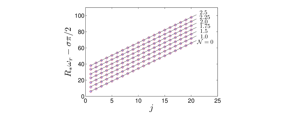
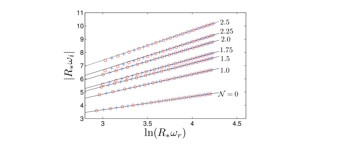
Figure 1: The axial (circles) and the polar (crosses) w-mode QNMs of the polytropic stars considered in Table 3 are shown. (a) $R_{*}\omega_{\rm r}-\sigma\pi/2$ is plotted against the mode number $j$, $j=1,2,3,...,20$. For clarity the data of each polytropic star are upward-shifted by 5, 10, 15, 20, 25, 30 for ${\cal N}=1,1.5,1.75,2.0,2.25,2.5$, respectively. (b) $|R_{*}\omega_{\rm i}|$ is plotted against $\ln(R_{*}\omega_{\rm r})$ for $5\leq j\leq 20$. The solid straight lines in (a) and (b) are the corresponding theoretical lines predicted by (40) and (41), respectively.

As introduced above, axial and polar oscillations are governed by two completely different formalisms. Therefore, it seems plausible that axial and polar w-mode QNMs would acquire different asymptotic behaviors. We have carried out numerical calculations to locate these QNMs for various stars, including polytropic stars (with EOS $p\propto\rho^{\gamma}$), quark stars (with EOS $p=(\rho-4B)/3$) and NSs constructed with several popular EOSs of nuclear matter, to examine relevant high-frequency behavior. The results obtained are in fact a bit surprising and encouraging as well. As shown in Fig. 1, where axial and polar w-mode QNMs of quark stars and polytropic stars are shown and analyzed, for a specific star these two kinds of w-mode QNMs lie on a common smooth curve star in the complex $\omega$-plane, which can be approximated by the following equations:

$$\omega_{{\rm r}}R_{*} = \pi j-\frac{(\widetilde{\theta}_{b}-\sigma\pi)}{2},$$ (9)

$$\omega_{{\rm i}}R_{*} = \frac{1}{2}\ln\left[r_{b}(R_{*})^{{\cal N}+2}\right]-(\frac{{\cal N}}{2}+1)\ln(\omega_{{\rm r}}R_{*}),$$ (10)

where $j=1,2,3,\ldots$ is the mode number labeling QNMs in order of increasing frequency, $\widetilde{\theta}_{b}$ and $r_{b}>0$ are real parameters dependent on the star, $\sigma=0(1)$ for axial (polar) w-mode, ${\cal N}\equiv 1/(\gamma-1)$ is the so-called polytropic index (${\cal N}=0$ for quark stars hereafter), and $R_{*}$ is the tortoise radius of the star.

The situation for realistic stars is less uniform and it is difficult to extract a generic asymptotic behavior for $\omega_{\rm i}$ (see Fig. 2). However, $\omega_{\rm r}$ still obeys an approximate equation similar to (9), namely

$$\omega_{\rm r}\widetilde{R}_{*}=\pi j-\frac{(\widetilde{\theta}_{b}-\sigma\pi)}{2}.$$ (11)

Here the parameter $\widetilde{R}_{*}$ is usually a bit less than $R_{*}$ and could have a mild dependence on $\omega$. Despite the lack of an explicit formula for $\omega_{\rm i}$, there is a universal relationship between the complex QNM frequencies of axial and polar w-modes:

$$\omega_{j}^{({\rm P})}=(\omega_{j}^{({\rm A})}+\omega_{j+1}^{({\rm A})})/2$$ (12)

and vice versa, where the superscripts P and A denote polar and axial modes, respectively. This equation holds asymptotically for large $j$ and works nicely irrespective of EOS of the star (including various nuclear matter EOSs, polytropic EOS and quark matter EOS). The main objective of the present paper is to establish a proper theory to explain these observed asymptotic behaviors, which will be the focus of the following sections. In fact, we will show how the values of $\widetilde{\theta}_{b}$ and $r_{b}$ for polytropic stars and quark stars can be obtained analytically.

III Wave equation for polar w-mode

The similarity between the asymptotic behaviors of the two kinds of w-mode is a bit surprising since they are in general governed by two entirely different sets of equations. The findings discussed in the last section strongly hint that axial and polar w-modes could actually be placed on an equal footing at least in the large-frequency limit. In this section we shall develop a HFA for polar w-modes under the inverse-Cowling approximation (ICA) Andersson et al. (1996); Wu and Leung (2007) to show that they can be described by a single second-order wave equation analogous to (2). To this end, we first introduce an alternative formalism of non-radial polar oscillations of compact stars suggested by Allen, Andersson, Kokkotas and Schutz Allen et al. (1998), referred to as AAKS formalism in the following discussion.

III.1 AAKS Formalism

In AAKS formalism polar oscillations of compact stars are described by two spacetime metric variables $F$, $S$ and one fluid perturbation variable $H$:

$$rF = h_{\theta\theta},$$ (13)

$$rS = h_{tt}-\frac{e^{\nu}}{r^{2}}h_{\theta\theta},$$ (14)

$$H = \frac{\delta p}{\rho+p},$$ (15)

where $h_{\alpha\beta}$ ($\alpha,\beta=t,r,\theta,\phi$) denotes the first-order perturbation in the metric, and $\delta p$ is the Eulerian variation in pressure Allen et al. (1998). These three physical quantities satisfy three second-order evolution equations plus one second-order time-independent (or equivalently frequency-independent) Hamiltonian constraint equation and one can use any three of these four equations to solve for $F$, $S$ and $H$. In this paper we shall use the two wave equations:

$$\omega^{2}S+\frac{d^{2}S}{dr_{*}^{2}}+\frac{2e^{\nu}}{r^{3}}\left[2\pi r^{3}(\rho+3p)+m-(n+1)r\right]S=-\frac{4e^{2\nu}}{r^{5}}\left[\frac{(m+4\pi pr^{3})^{2}}{r-2m}+4\pi\rho r^{3}-3m\right]F\,,$$ (16)

$$\omega^{2}F+\frac{d^{2}F}{dr_{*}^{2}}+\frac{2e^{\nu}}{r^{3}}\left[2\pi r^{3}(3\rho+p)+m-(n+1)r\right]F=-2\left[4\pi r^{2}(p+\rho)-e^{-\lambda}\right]S+8\pi(\rho+p)re^{\nu}\left(1-\frac{1}{C_{s}^{2}}\right)H\,,$$

plus the Hamiltonian constraint:

$$0 = \frac{d^{2}F}{dr_{*}^{2}}-\frac{e^{(\nu+\lambda)/2}}{r^{2}}(m+4\pi r^{3}p)\frac{dF}{dr_{*}}+\frac{e^{\nu}}{r^{3}}[12\pi r^{3}\rho-m-2(n+1)r]F$$ (18)

$$-re^{(\nu+\lambda)/2}\frac{dS}{dr_{*}}+\left[8\pi r^{2}(p+\rho)-(n+3)+\frac{4m}{r}\right]S+\frac{8\pi r}{C_{s}^{2}}e^{\nu}(\rho+p)H$$

to develop a second-order wave equation for polar w-mode. In these equations $n=(l-1)(l+2)/2$, and $C_{s}$ is the sound speed in the stellar fluid.

III.2 Inverse-Cowling approximation

It is commonly accepted that polar w-mode oscillations are oscillations in spacetime and fluid elements are to certain extent spectators. Hence, it is reasonable to expect that polar w-mode QNMs could be reproduced under the so-called ICA where certain fluid perturbations (e.g. fluid displacements or pressure variation) are neglected Andersson et al. (1996); Wu and Leung (2007). In fact, it has been shown that ICA assuming zero Lagrangian pressure variation can produce quantitatively correct result Wu and Leung (2007). Here we propose another version of ICA, namely zero Eulerian pressure variation (i.e., $\delta p=0$), to derive a valid wave equation for polar w-mode QNMs.

From (III.1) and (18), we have:

$$8\pi re^{\nu}\delta p=\omega^{2}F+\frac{e^{(\nu+\lambda)/2}}{r^{2}}(m+4\pi pr^{3})\frac{dF}{dr_{*}}+\frac{e^{\nu}}{r^{3}}(3m+4\pi pr^{3})F+re^{-(\nu+\lambda)/2}\frac{dS}{dr_{*}}+(n+1)S.$$ (19)

Under our ICA scheme, $\delta p=0$, and consequently Eq. (19) can be rewritten in the following way:

$$F=-\frac{e^{(\nu+\lambda)/2}(m+4\pi pr^{3})}{\omega^{2}r^{2}}\frac{dF}{dr_{*}}-\frac{e^{\nu}(3m+4\pi pr^{3})}{\omega^{2}r^{3}}F-\frac{re^{-(\nu+\lambda)/2}}{\omega^{2}}\frac{dS}{dr_{*}}-\frac{n+1}{\omega^{2}}S.$$ (20)

This equation, together with (16), can lead to a single wave equation in $S$.

III.3 High-frequency approximation

We note that the frequencies of w-mode are at least a few times higher than that of $f$-mode, which is proportional to $(M/R^{3})^{1/2}\sim\overline{\rho}^{1/2}$, with $\overline{\rho}$ being the average density of the star. As a result, terms of the order $\overline{\rho}^{1/2}/\omega$ are small for w-mode QNMs and can be neglected for high-order modes. Based on this observation and (20), we have developed a systematic power expansion in $1/\omega$ for $F$. Hence, the contribution of $F$ to (16) can be included perturbatively, leading to an accurate scheme to solve for $S$. The details of such perturbation scheme are provided in Appendix A for reference. However, since we are interested in the high-frequency asymptotic behavior of polar w-mode, we adopt the lowest order HFA where the contribution of $F$ to (16) is neglected completely to obtain a single wave equation for $S$:

$$\left[\frac{d^{2}}{dr_{*}^{2}}+\omega^{2}-V_{\rm p}(r_{*})\right]S(r_{*})=0\,$$ (21)

with

$$V_{\rm p}(r_{*})=\left\{\begin{array}[]{lr}\displaystyle{\frac{e^{\nu}}{r^{3}}}\left[l(l+1)r-4\pi r^{3}(\rho+3p)-2m\right],&\hskip 14.22636ptr<R;\\ \displaystyle{\frac{e^{\nu}}{r^{3}}}\left[l(l+1)r-2M\right],&\hskip 14.22636ptr\geq R.\end{array}\right.$$ (24)

This polar w-mode wave equation is identical to the wave equation for the axial mode, (2), except for the functional form of the potential term. We will see in the following discussion that such similarity between the governing equations of these two kinds of w-mode wave is in fact the origin of the peculiar asymptotic behavior observed in Sect. II.

To gauge the accuracy of HFA and examine the validity of (21), we located the first ten polar w-mode QNMs with (21) and compared the numerical results with the exact values in Tables 1 and 2 for a polytropic star (EOS: $p=100\rho^{2}$) with a compactness $0.297$, and a realistic star (EOS: APR2 Akmal et al. (1998)) with a compactness $0.196$, respectively. The numerical results of $\omega$ are given in units of $M^{-1}$. From the numerical results, it is obvious that the error of HFA decreases with increasing $\omega$. Therefore, the HFA can indeed provide us accurate results for high-order modes.

IV Asymptotic Behavior of w-modes for model Stars

In the above discussion we have shown that both axial and polar w-mode QNMs of compact stars are governed by a Klein-Gordon type wave equation:

$$\left[\frac{d^{2}}{dr_{*}^{2}}+\omega^{2}-V(r_{*})\right]\psi(r_{*})=0,$$ (25)

where $V=V_{{\rm a}}\,(V_{\rm p})$ and $\psi=\psi_{{\rm a}}\,(S)$ for axial (polar) case. Despite the fact that the form of (25) is similar to the Regge-Wheeler equation and the Zerilli equation describing GW propagation around BHs Regge and Wheeler (1957); Zerilli (1970), the potential $V$ has non-trivial dependence on density and pressure. To see how such dependence could affect the asymptotic behavior of relevant QNMs, in this section we focus our attention on stars with simple analytic EOS, namely polytropic stars and quark stars described by the simplest MIT bag model with zero strange quark mass.

IV.1 Locating QNMs

One usual way to locate QNMs is as follows. For any specific $\omega$, we first find a function $f(\omega,r_{*})$ satisfying the regularity condition $f\sim r_{*}^{l+1}$ as $r_{*}\rightarrow 0$ and a function $g(\omega,r_{*})$ satisfying the outgoing condition $g\sim\exp(i\omega r_{*})$ as $r_{*}\rightarrow\infty$. QNMs are then located when the Wronskian of $f(\omega,r_{*})$ and $g(\omega,r_{*})$ vanishes, i.e.,

$$W(f,g;\omega)\equiv f(\omega,r_{*})\frac{d}{dr_{*}}g(\omega,r_{*})-g(\omega,r_{*})\frac{d}{dr_{*}}f(\omega,r_{*})=0,$$ (26)

and the corresponding eigenfunction is proportional to $f(\omega,r_{*})$ (or equivalently $g(\omega,r_{*})$).

In the high-frequency domain the asymptotic expression of $f(\omega,r_{*})$, $g(\omega,r_{*})$ and $W(\omega)$ can be derived under the standard WKB approximation, and hence an approximate expression of QNM frequencies can be derived as well Ching et al. (1995, 1996). As in other applications of the WKB approximation, due attention has to be placed on the singular points of the potential, e.g., points at which the potential (or the derivatives of the potential) are discontinuous. For polytropic stars and quark stars, $V(r_{*})$ is well behaved except at the stellar surface. We shall show in the following analysis how the reflection of GW at the stellar surface could dominate the asymptotic behavior of w-mode QNMs.

IV.2 WKB analysis

Adopting the methods discussed in Berry (1982); Slavyanov (1996), we have developed a systematic WKB analysis for both $f$ and $g$ (see Zhang (2009) for details). In the high-frequency limit, the dominant parts in $f$ and $g$ are given respectively by

$$f(r_{*},\omega\rightarrow\infty)=\omega r_{*}j_{l}(\omega r_{*}),\hskip 28.45274pt0\leq r_{*}\leq R_{*},$$ (27)

and

$$g(r_{*},\omega\rightarrow\infty)=\left\{\begin{array}[]{lr}\exp\left[i\omega(r_{*}-R_{*})\right]+{\cal R}\exp\left[-i\omega(r_{*}-R_{*})\right],&1/\omega\ll r_{*}<R_{*};\\ (1+{\cal R})\exp\left[i\omega(r_{*}-R_{*})\right],&R_{*}\leq r_{*}<\infty.\end{array}\right.$$ (30)

Here ${\cal R}$ is the standard reflection coefficient as defined in Berry (1982). In particular, if the potential $V(r_{*})$ has a discontinuity in $d^{N}V/dr_{*}^{N}$ ($N=0,1,2,\ldots$), ${\cal R}=a\omega^{-(N+2)}$, with

$$a=-\left(\frac{i}{2}\right)^{N+2}\lim_{\varepsilon\rightarrow 0^{+}}\left[\frac{d^{N}V(r_{*})}{dr_{*}^{N}}|_{r_{*}=R_{*}+\varepsilon}-\frac{d^{N}V(r_{*})}{dr_{*}^{N}}|_{r_{*}=R_{*}-\varepsilon}\right].$$ (31)

Detailed derivation of the above result can be found in Berry (1982).

The asymptotic eigenvalue equation for w-mode QNMs is then obtained by setting the Wronskian of $g(r_{*},\omega\rightarrow\infty)$ and $f(r_{*},\omega\rightarrow\infty)$ to zero:

$$b\omega^{-(N+2)}=\exp({-i2\omega R_{*}}),$$ (32)

where $b\equiv r_{b}\exp(i\theta_{b})=(-1)^{l+1}a$ with $r_{b}>0$ and $\theta_{b}$ being two real constants. This equation can be solved readily, yielding

$$\omega_{j}\approx\frac{1}{2R_{*}}\left\{2\pi j-\theta_{b}-i\left[(N+2)\ln\frac{2\pi j-\theta_{b}}{2R_{*}}-\ln r_{b}\right]\right\},$$ (33)

where $j\gg 1$ is a positive integer and the approximation $|\omega|\simeq|\omega_{\rm r}|$ has been used.

It is obvious that Eq. (33) indeed leads to the asymptotic behavior of w-mode summarized in Sect. II as long as $N$ is equal to the polytropic index ${\cal N}$. In the following discussion we shall show that this is the case for ${\cal N}=0,1,2,\ldots$. More importantly, Eq. (33) can be generalized to include cases with non-integral values of ${\cal N}$. Before diving into detailed calculation of $b$, several useful features of (33) are worthy of remark. Firstly, $\omega_{\rm r}$ of the $j$-th and $({j+1})$-th eigenfrequencies are spaced by $\pi/R_{*}$. Secondly, $\omega_{\rm i}$ depends linearly on the logarithm of $\omega_{\rm r}$. The above features both hold for axial and polar high-frequency w-modes. In addition, since the leading discontinuity in the potential $V_{{\rm a}}$ or $V_{\rm p}$ is usually caused by the $\pm 4\pi e^{\nu}\rho$ term, the expression of $b$ has a minus sign difference between the axial and the polar cases. The phases of $b$ for the axial and polar cases thus differ by $\pi$, leading to a shift of $\pi/(2R_{*})$ in $\omega_{\rm r}$. All these features are consistent with our numerical results presented in Sect. II.

IV.3 Application to model stars

To make our discussion concrete and physical, we apply our analysis to quark stars and polytropic stars, which are described by EOSs with analytic forms. It is readily shown that the potential and the derivatives of the potential for such stars are continuous except at the stellar surface. In the following we will show how the values of $N$ and $b$ can be expressed in terms of the physical parameters of the star.

For a quark star with the MIT Bag Model EOS ($\rho=3p+4B$, with $B$ being the bag constant), the star surface is defined at the point where the pressure vanishes. However, the density there is equal to $4B$ and does not vanish. Therefore, the potential has a direct discontinuity at the surface of the star, i.e., the $N=0$ limit of (31), and straightforward calculation shows that

$$b = (-1)^{l+\sigma}4B\pi\left(1-\frac{2M}{R}\right).$$ (34)

We now turn our attentions to polytropic stars with EOS given explicitly by $p=\kappa\rho^{1+1/{\cal N}}$, where $\kappa$ is a constant. Again, it is easy to see from TOV equations that the variables $m$, $\rho$, $p$ and $\nu$ of polytropic stars are all analytic functions inside the star and hence our theory applies. Near the surface of the star, following directly from the TOV equations, the density and the pressure behave respectively as Lindblom and Detweiler (1983):

$$p = \alpha(R_{*}-r_{*})^{{\cal N}+1},$$ (35)

$$\rho = \beta(R_{*}-r_{*})^{\cal N},$$ (36)

where

$$\beta = \left[\frac{1}{\kappa({\cal N}+1)}\frac{M}{R^{2}}\right]^{\cal N},$$ (37)

$$\alpha = \kappa\beta^{1+1/{\cal N}}.$$ (38)

We first consider a simple case where ${\cal N}$ is equal to a positive integer $N$. Then the lowest order discontinuity appears in the $N$-th derivative of the potential at the surface and the coefficient $b$ can be found explicitly:

$$b=(-1)^{l+\sigma}\pi\Gamma({\cal N}+1)\left(1-\frac{2M}{R}\right){\left[\frac{-iM}{2\kappa({\cal N}+1)R^{2}}\right]}^{{\cal N}},$$ (39)

where $\Gamma(z)$ is the gamma function. It is interesting to note that Eq. (39) in fact includes (34) as the special case ${\cal N}=0$.

It follows directly from the asymptotic analysis developed above that for $j\gg 1$

$$\omega_{{\rm r}}R_{*} = \pi j-\frac{\left(\widetilde{\theta}_{b}-\sigma\pi\right)}{2},$$ (40)

$$\omega_{{\rm i}}R_{*} = -(\frac{{\cal N}}{2}+1)\ln(\omega_{r}R_{*})+\frac{1}{2}\ln\left[r_{b}(R_{*})^{{\cal N}+2}\right],$$ (41)

with

$$\widetilde{\theta}_{b}\equiv{\theta}_{b}+\sigma\pi=\left(-l-\frac{{\cal N}}{2}\right)\pi\,.$$ (42)

It is obvious that the forms of (40) and (41) agree with the numerical results summarized in Sect. II. Most interestingly, Eqs. (39), (40) and (41) can be readily generalized to non-integral values of ${\cal N}$ by method of analytic continuation. Thus, we have established a generic and unified asymptotic behavior for polytropic stars and quark stars as well.

IV.4 Numerical results

To further examine the validity and accuracy of our method, we have calculated the exact eigenfrequencies for w-mode QNMs of several model stars (including one quark star and six polytropic stars whose physical parameters are tabulated in Table 3 for reference) and showed the results in Fig. 1. It is clearly shown in these figures that the asymptotic behavior of w-mode QNMs agrees nicely with the theoretical results derived above. For example, the spacing in $\omega_{\rm r}$ between two successive QNMs of the same polarity is close to $\pi/R_{*}$. There is one axial (polar) QNM at the midpoint of the line joining two neighboring polar (axial) QNMs (i.e. Eq. (12)). Besides, $\omega_{\rm i}$ depends linearly on $\ln j$. These features are just the direct consequence of (40) and (41).

On the other hand, the coefficient $b$ for each case can be calculated from (39) with the physical parameters tabulated in Table 3. Substituting the so-obtained value of $b$ (see Table 3) into (40) and (41), we can determine both $\omega_{{\rm r}}$ and $\omega_{{\rm i}}$ for $j\gg 1$ without using any unknown free paramter. To further verify our theory, we have fitted exact values of $\omega_{{\rm r}}$ and $\omega_{{\rm i}}$ with the following functions:

$$\omega_{{\rm r}}R_{*} = c_{1}j+c_{0},$$ (43)

$$\omega_{{\rm i}}R_{*} = d_{1}\ln(\omega_{r}R_{*})+d_{0},$$ (44)

with $c_{1}$, $c_{0}$, $d_{1}$ and $d_{0}$ being adjustable parameters to yield the best fit. The theoretical values of these parameters (see (39), (40) and (41)) and the values obtained from the best fit to the w-modes (from the $11$-th to the $20$-th modes) are listed in Tables 4 (values of $c_{1}$, $c_{0}$) and 5 (values of $d_{1}$, $d_{0}$). It is obvious that our analysis works nicely in all cases. The numerical values of both $c_{1}$ and $d_{1}$ are close to their theoretical ones. For the case of $c_{0}$ and $d_{0}$, the errors are larger, especially for the former. This is expected as small errors in the slope would result in much larger errors in the intercept in the process of extrapolation. Therefore, as a remedial action, we have first set $c_{1}$ and $d_{1}$ to their theoretical values and substituted the eigenfrequency of the $20$-th w-mode into (43) and (44) to compute $c_{0}$ and $d_{0}$ directly (the numeric results enclosed in brackets in Tables 4 and 5). It is clear that this modified method can improve the accuracy to certain extent.

V Unified approach to w-modes

From the asymptotic analysis on w-modes developed above we see that the asymptotic behaviors of w-modes are mainly determined by the most singular part in the potential, which is responsible for reflection of GWs at high frequencies. Apart from the trivial centrifugal barrier that has been duly considered by adopting the solution $f\propto j(\omega r_{*})$, there are three other terms in the potential which are proportional to $\rho$, $p$ and $m$, respectively. As usual, the effect of $p$ is much less than that of $\rho$. Moreover, $m$ is an integral over the $\rho$ term (see (8)) and should be less singular than $\rho$. Hence, it is reasonable to argue that both the contributions of $p$ and $m$ to the potential are small at high frequencies. Once the terms proportional to $p$ and $m$ are neglected in the potential, $V_{{\rm a}}$ and $V_{\rm p}$ are almost identical except for a sign difference in the term proportional to $\rho$. More importantly, such argument should work irrespective of the EOS of a star. We therefore propose to use the following unified approach to w-modes:

$$\left[\frac{d^{2}}{dr_{*}^{2}}+\omega^{2}-V(r_{*})\right]\psi(\omega,r_{*})=0,$$ (45)

with

$$V(r_{*})=\left\{\begin{array}[]{lr}\displaystyle{\frac{e^{\nu}}{r^{3}}}\left[l(l+1)r+(-1)^{\sigma}4\pi r^{3}\rho\right],&\hskip 14.22636ptr<R;\\ \\ \displaystyle{\frac{1}{r^{3}}}l(l+1)(r-2M),&\hskip 14.22636ptr\geq R.\end{array}\right.$$ (49)

Thus, the two kinds of w-modes are cast in a symmetrical description.

We have tested the validity of our proposal by comparing the numerical results of the w-mode QNM eigenfrequencies obtained from the above approximate wave equation with the exact values in Tables 6 (axial case) and 7 (polar case). The star under consideration is a realistic NS with EOS A (Pandharipande, 1971a), which has a compactness of $0.27$ and a central density $\rho_{c}=2.227\times 10^{-3}$. The w-modes listed in the tables are the $3$-rd to $12$-th modes. One can see that the unified approach works accurately for both kinds of w-mode. The percentage error in $\omega_{\rm r}$ and $\omega_{\rm i}$ is less than $1\%$ in most cases and decreases with increasing order. Thus, the validity of the approximate form of the potential in (49) is justified. As a result, w-modes of both polarities can be cast into a unified description.

VI Generalization to Realistic Neutron Stars

VI.1 Numerical result

It is not easy to generalize the method established above to analyze the w-modes of NSs characterized by realistic EOSs of nuclear matter for the following reasons. First, such EOSs are usually given in the form of discrete data points and methods of interpolation are needed in order to generate the function $p(\rho)$ (see, e.g., Arnett and Bowers (1977)). It is likely that artificial discontinuities in the potential (or its derivatives) may develop when $p(\rho)$ so generated is used as the input to solve the TOV equations describing the static configuration of a compact star. These artificial discontinuities could then lead to extra reflections of GW and obscure numerical results of high-order QNMs and the related theoretical study as well. Second, the polytropic index of nuclear matter is in general density-dependent. However, as shown in the previous section, the polytropic index is a crucial factor in the asymptotic behavior of w-mode QNM. Except for GWs with very high frequencies, reflections occurring at interfaces other than the stellar surface are characterized by different polytropic indices, leading to more uncertainties in the asymptotic behavior of realistic NSs.

Instead of deriving the asymptotic behaviors of w-modes for realistic compact stars from first principles, we have gathered some empirical rules for high-frequency w-mode QNMs based on numerical studies carried out for numerous stellar models, including models A Pandharipande (1971a), C Pandharipande (1971b), three models (AU, UU and UT) proposed in Wiringa et al. (1988), and models APR1 and APR2 proposed in Akmal et al. (1998). In particular, we have constructed NSs based on the two analytic EOS proposed by Haensel and Potekhin Haensel and Potekhin (2004), which can well approximate FPS EOS Pandharipande and Ravenhall (1989) and SLy EOS Douchin and Haensel (2001) of realistic neutron-star matter. More importantly, these analytic EOS are free from artificial discontinuities due to interpolation of discrete data points and can facilitate theoretical analysis. As a representative example to illustrate our discussion, we show in Fig. 2 the w-mode QNMs of two NSs obeying the analytic SLy EOS with compactness ${\cal C}=0.306,\,0.228$, from which one can see the following features. First, despite the fact that $\omega_{\rm r}$ no longer follows (40), it obeys a modified version of (40), namely (11), where $R_{*}$ is replaced with $\widetilde{R}_{*}$. Strictly speaking, $\widetilde{R}_{*}$ also has a mild frequency dependence, but such dependence is not obvious in the frequency range shown in Fig. 2. Second, $\omega_{{\rm i}}R_{*}$ is no longer a linear function of $\ln(\omega_{{\rm r}}R_{*}$). The graph $|\omega_{{\rm i}}R_{*}|$ versus $\ln(\omega_{{\rm r}}R_{*}$) shown in Fig. 2 displays a frequency-dependent slope. The slope of the graph increases from about 1.3 (1.3) to about 1.4 (1.9) for the case ${\cal C}=0.306$ (${\cal C}=0.228$) when $j$ goes from 5 to 20. Generally speaking, the slope demonstrates a greater dependence on frequency for NSs with smaller compactness. Third, although for realistic stars both $\omega_{\rm r}$ and $\omega_{\rm i}$ do not follow (40) and (41), the asymptotic behavior Eq. (12) still holds. Hence, axial and polar w-modes are located on the same smooth curve and evenly alternate with each other in the high-frequency regime. In the following we try to explain the above findings in a semi-quantitative way based on the asymptotic analysis developed for polytropic stars.

VI.2 Physical picture

First of all, it is instructive to associate such asymptotic behavior of w-mode QNMs with the physical structure and the EOS of realistic NSs. As is well known, a typical realistic NS consists of a core with supernuclear densities (i.e. $\rho\geq 2.8\times 10^{14}\,{\rm gm}\,{\rm cm}^{-3}$), and a thin crust at subnuclear densities. The crust can be further divided into an inner part and an outer part by the neutron drip density $\rho\approx 4\times 10^{11}\,{\rm gm}\,{\rm cm}^{-3}$. Due to the effect of neutron drip, stellar matter softens significantly and the adiabatic index $\Gamma$, a typical measure of stiffness defined by

$$\Gamma=\left(1+\frac{p}{\rho}\right)\frac{\rho}{p}\frac{dp}{d\rho}\,,$$ (50)

decreases abruptly from about 1.4 to about 0.4 near the neutron drip density. On the other hand, at the crust-core interface nuclei disappear and nuclear matter there consequently becomes particularly stiff owing to the repulsive part of short range nuclear force. Correspondingly, $\Gamma$ experiences a sharp rise from about 1.4 to about 3 around the density $\rho\sim 2\times 10^{14}\,{\rm gm}\,{\rm cm}^{-3}$. These softening and stiffening of nuclear matter give rise to huge and rapid changes in the density profile in the inner crust, which typically has a thickness of only about a few percent of the stellar radius. For GWs with wavelengths greater than the thickness of the inner crust, these drastic changes in the density effectively lead to discontinuities in the scattering potential $V$ and its derivatives as well. Hence, strong reflections of GWs are expected to occur at the core-crust interface and such a mechanism indeed attributes to formation of QNMs.

VI.3 Semi-quantitative analysis

As mentioned above, for a realistic NS, GWs are reflected not only at the stellar surface but also from other abrupt changes in $\rho$ inside the star. In general, the reflection coefficient ${\cal R}$ in (30) can be obtained from the leading term in Eq. (10) of Ref. Berry (1982), which yields:

$${\cal R}=\frac{\exp(-2i\omega{R}_{*})}{4\omega^{2}}\int_{0}^{\infty}dr_{*}\,\frac{dV}{dr_{*}}\exp(2i\omega r_{*})\,,$$ (51)

where in $V(r)$ the trivial centrifugal barrier has been excluded. This equation is generally valid and reduces to (31) if $V$ (or its $N$-th order derivative) has a step discontinuity at $r_{*}=R_{*}$. It can be clearly seen from (49) that the potential $V$ is dominated by the density term $\rho$. Hence, the reflection coefficient $\cal R$ is proportional to the Fourier transform of ${d\rho}/{dr_{*}}$.

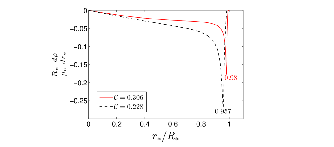
Figure 3: $d\rho/dr_{*}$ (normalized by $\rho_{c}/R_{*}$, with $\rho_{c}$ being the density at the center of the star) is plotted against $r_{*}$ (normalized by $R_{*}$) for two realistic stars obeying the analytic SLy EOS proposed in Ref. Haensel and Potekhin (2004) with compactness ${\cal C}=0.306,\,0.228$. As labelled in the graphs, $|d\rho/dr_{*}|$ attains maximum at $r_{*}=0.98R_{*}\,(0.957R_{*})$ for the case ${\cal C}=0.306\,(0.228)$.

In Fig. 3 we show ${d\rho}/{dr_{*}}$ versus $r_{*}$ for the two NSs constructed with the analytic SLy EOS Haensel and Potekhin (2004). It is interesting to see that there is a sharp peak in $|{d\rho}/{dr_{*}}|$ at $r_{*}=R_{m}$ near the surface of the star. Generally speaking, $R_{m}/R_{*}$ increases slowly while the width of the peak decreases with increasing compactness. This peak obviously reflects the abrupt change in the stiffness of nuclear matter around the core-crust interface. In fact, it can be argued that $R_{m}\cong R_{2}$, where at $r_{*}=R_{2}$ the adiabatic index $\Gamma$ equals 2 (see Appendix B and the data shown in Table 8).

For QNMs with wavelengths much longer than the width of the peak, ${d\rho}/{dr_{*}}$ can be well approximated by a $\delta$-function. Following directly from standard theory of asymptotic expansion of Fourier integrals (see, e.g., Bleistein and Handelsman (1986)), the leading behavior of the reflection coefficient is

$${\cal R}\sim\frac{a_{0}(\omega)}{\omega^{2}}\exp\left[2i\omega(R_{m}-{R}_{*})\right]\,,$$ (52)

where $a_{0}(\omega)$ approaches a constant at low frequencies and decreases rapidly if $1/|\omega|$ is much smaller than the width of the peak in $|{d\rho}/{dr_{*}}|$. Apart from this leading term, due to the asymmetry in $|{d\rho}/{dr_{*}}|$ around $r_{*}=R_{m}$, there are other sub-dominant terms in the the reflection coefficient, leading to the following asymptotic of ${\cal R}$:

$${\cal R}\approx\left(\frac{a_{0}}{\omega^{2}}+\frac{a_{1}}{\omega^{3}}+\frac{a_{2}}{\omega^{4}}+\ldots\right)\exp\left[2i\omega(R_{m}-{R}_{*})\right].$$ (53)

Physically speaking, the coefficients $a_{0}(\omega)$, $a_{1}(\omega)$ and $a_{2}(\omega)$ measure the discontinuities in $\rho$, ${d\rho}/{dr_{*}}$ and ${d^{2}\rho}/{dr_{*}^{2}}$ around the point $r_{*}=R_{m}$, respectively. As in the case of $a_{0}(\omega)$, $a_{1}(\omega)$ and $a_{2}(\omega)$ decreases rapidly if $1/|\omega|$ is much smaller than the typical length scale associated with the corresponding discontinuity.

VI.4 Asymptotic behavior

Recalling the asymptotic eigenvalue equation (32) for polytropic stars and taking (53) into consideration, we can show that for realistic stars the w-mode QNMs are asymptotically given by the solution of the equation:

$${\cal R}(\omega)\approx(-1)^{l+1}\exp({-i2\omega{R}_{m}}).$$ (54)

Since the most singular part of the potential is dominated by the $\rho$ term, from (31) and (49) we see that the generalized reflection coefficients for axial and polar w-modes should have the same frequency dependence but with a sign difference. Therefore, the two eigenvalue equations for axial and polar w-modes can be unified into one single equation:

$${\cal R}_{\rm a}(\omega)\approx(-1)^{l+1+\sigma}\exp({-i2\omega_{\rm r}{R}_{m}})\exp(2\omega_{\rm i}{R}_{m}),$$ (55)

with ${\cal R}_{\rm a}$ being the reflection coefficient of the axial w-mode, and $\sigma=0\,(-1)$ for the axial (polar) case. In the asymptotic region, ${\cal R}_{\rm a}$ is further assumed to have a constant phase, i.e., ${\cal R}_{\rm a}(\omega)\approx\exp(i\theta_{\rm a})|{\cal R}_{\rm a}(\omega)|$, Eq. (55) then leads to:

$$\omega_{\rm r}{R}_{m} = \pi j-\frac{\theta_{\rm a}-(l+1+\sigma)\pi}{2},$$ (56)

$$\omega_{\rm i}{R}_{m} = \frac{1}{2}\ln(|{\cal R}_{\rm a}(\omega)|).$$ (57)

Upon equating $\theta_{\rm a}-(l+1)\pi$ with $\widetilde{\theta}_{b}$, Eq. (56) agrees nicely with (11), which is an empirical relation obtained from numerical data such as those shown in Fig. 2, provided that $\widetilde{R}_{*}=R_{m}$. Our argument readily provides the numerical value of $\widetilde{R}_{*}$ in (11) a proper physical interpretation. $\widetilde{R}_{*}$ is actually the tortoise coordinate of the point at which $|d\rho/dr_{*}|$ attains a maximum. In addition, $\widetilde{R}_{*}$ is also close to the tortoise coordinate of the point where the adiabatic index is 2 and nuclear matter becomes stiff due to the disappearance of individual nuclei. This point is confirmed by the numerical data shown in Table 8.

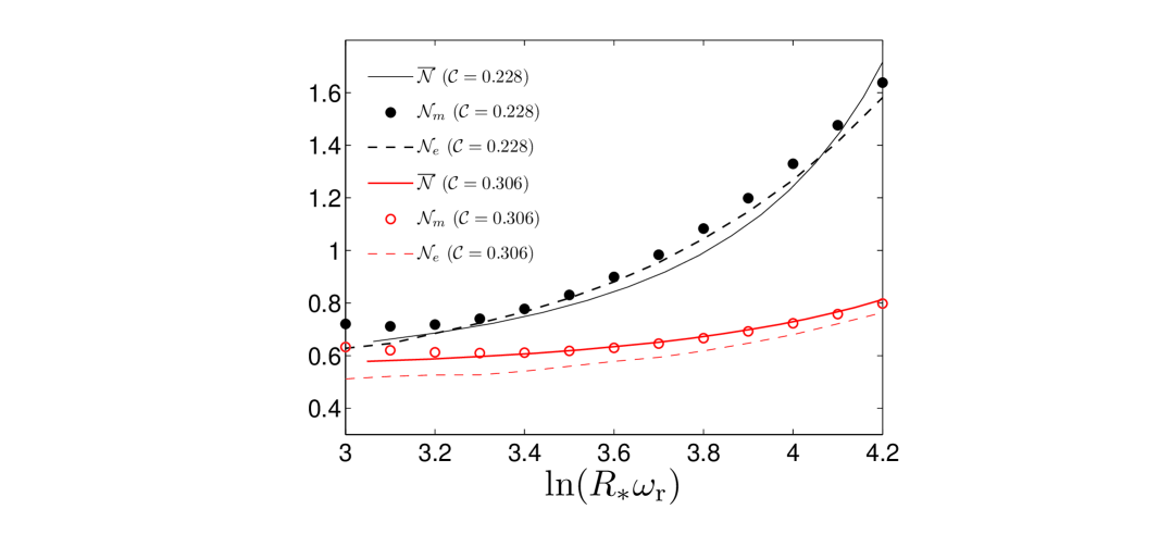
Figure 4: $\overline{{\cal N}}$, ${\cal N}_{m}$ and ${\cal N}_{e}$ are plotted against $\ln(R_{*}\omega_{\rm r})$ for two SLy stars with ${\cal C}=0.228,0.306$, respectively.

As suggested in (57), $\omega_{\rm i}$ depends crucially on the magnitude of the reflection coefficient ${\cal R}_{\rm a}(\omega)$. For the cases of polytropic stars and quark stars, ${\cal R}_{\rm a}(\omega)\propto\omega^{-({\cal N}+2)}$, leading directly to (41), and the plot of $|\omega_{\rm i}{R}_{*}|$ versus $\ln(\omega_{\rm r}{R}_{*})$ is a straight line with a slope $m_{s}=({\cal N}+2)/2$. In the cases of realistic NS, the polytropic index ${\cal N}$ as well as the adiabatic index $\Gamma$ depend on density $\rho$. It is therefore reasonable to expect that the plot of $\omega_{\rm i}$ versus $\ln\omega_{\rm r}$ is no longer a straight line. This is in agreement with the result shown in Fig. 2. As a matter of fact, the slope of the curve, $m_{s}(\omega_{\rm r})\equiv[{\cal N}_{m}(\omega_{\rm r})+2]/2$, increases gradually with $\omega_{\rm r}$ and the trend is more obvious for the star with ${\cal C}=0.228$. In Fig. 4 the value of ${\cal N}_{m}$ for the is plotted against $\ln(\omega_{\rm r}{R}_{*})$ two SLy stars. As shown in the following discussion, ${\cal N}_{m}$ so obtained could indeed measure the variation of the polytropic index ${\cal N}$ near the stellar surface.

Since the reflection of GWs mainly takes place around the stellar surface, we define the average value of $\Gamma$ over a surface layer with a thickness measured by the wavelength $\lambda=2\pi/\omega_{\rm r}$, namely:

$$\overline{\Gamma}=\frac{1}{\Delta}\int_{R_{*}-\Delta}^{R_{*}}\Gamma(r_{*})dr_{*}\,,$$ (58)

where $\Delta=\eta\lambda$ with $\eta=0.61\,(0.7)$ for the star with ${\cal C}=0.306\,(0.228)$ in our calculations. In Fig. 4 we compare the values of ${\cal N}_{m}$ with $\overline{{\cal N}}$ defined by

$$\overline{{\cal N}}\equiv\frac{1}{\overline{\Gamma}-1}.$$ (59)

It is interesting to note that $\overline{{\cal N}}$ can indeed approximate ${\cal N}_{m}$ nicely. Thus, the link between the asymptotic behavior of w-mode QNMs and the EOS of the nuclear matter distributed within around one wavelength about the stellar surface is clearly displayed.

On the other hand, the asymptotic expansion of the reflection coefficient in (53) could also cast light on the variation of the slope $m(\omega_{\rm r})$. For GWs with wavelengths longer than the thickness of the crust, they get reflected from the narrow peak in $|d\rho/dr_{*}|$ around the core-crust interface. Such reflection is measured by the term $a_{0}/w^{2}$ in the expansion of $\cal R$. However, as shown in (53), there are other contributions $a_{1}/w^{3}$ and $a_{2}/w^{4}$ due to reflections resulting from discontinuities of higher orders. Each of these terms alone leads to an effective slope 1, 1.5 and 2, respectively. On the other hand, for GWs with wavelengths less than the width of the peak, the value of $a_{0}$ decreases markedly. Thus, we expect that the frequency-dependent slope of the graph $|\omega_{{\rm i}}R_{*}|$ versus $\ln(\omega_{{\rm r}}R_{*}$) in Fig. 2 increases with frequency gradually from 1 to 1.5, and then to 2. Such increase in the slope is expected to be more pronounced if the peak in $d\rho/dr_{*}$ is broader. Our conjecture indeed agrees with the numerical data qualitatively.

Furthermore, we define an effective (frequency-dependent) polytropic index ${\cal N}_{e}$ by:

$${\cal N}_{e}=-\frac{\partial\ln|{\cal R}_{\rm a}|}{\partial\ln\omega_{\rm r}}-2\,.$$ (60)

For polytropic stars ${\cal N}_{e}$ reduces to the standard polytropic index ${\cal N}$. As shown in Fig. 4, the trend of ${\cal N}_{e}$ (minor oscillations in ${\cal N}_{e}$ have been suppressed) agrees qualitatively with those of ${\cal N}_{m}$ and $\overline{{\cal N}}$. This once again demonstrates the close relationship between the high-frequency behavior of w-mode QNMs and the mass distribution of a NS.

VI.5 Methods relating QNMs

In spite of the complexity in the situation of realistic NSs, the relationship between the axial and polar w-modes for these stars is identical to that for polytropic stars. Due to the sign difference in the reflection coefficients of axial and polar GWs, $\omega_{\rm r}$ of axial and polar w-mode frequencies, with the same mode index $j$, differ approximately from each other by $\pi/(2\widetilde{R}_{*})$. Hence, the real part of a polar w-mode eigenfrequency lies in the middle of two axial w-modes and vice versa. The difference of $\omega_{\rm r}$ leads to the difference in $\omega_{\rm i}$ through (57). Therefore, the imaginary part of a polar w-mode eigenfrequency should also lies approximately in the middle of two axial w-modes.

Based on the relationship between the two types of w-mode, two methods are proposed here to derive approximate polar w-mode eigenfrequencies from the corresponding axial w-mode eigenfrequencies. The first method is to approximate $\omega$ of the $j$-th polar w-mode QNM with the mean value of the eigenfrequencies of its two neighboring axial w-mode QNMs of the same $l$, i.e., $\omega_{j}^{(P)}=(\omega_{j}^{(A)}+\omega_{j+1}^{(A)})/2$. Besides, from (56) it is obvious that the asymptotic behaviors of polar w-modes with $l=l_{0}$ and axial w-modes with $l=l_{0}+1$ are the same. Hence, it is possible to approximate the frequency of a polar w-mode with $l=l_{0}$ with that of an axial w-mode with the same mode order but $l=l_{0}+1$. As numerical calculations of axial w-mode eigenfrequencies are usually much easier and faster than polar w-mode calculations, the two methods mentioned above are deemed useful to provide quick ways to locate approximately polar w-mode QNMs. As an example to illustrate our method, we consider the w-mode QNMs of a model C NS (with compactness ${\cal C}=0.186$ and central density $\rho_{c}=8.752\times 10^{-4}$) and evaluate approximate polar w-mode frequencies (from the $5$-th to $14$-th modes) for the case $l_{0}=2$ using these two methods. The approximate results so obtained are listed and compared with the exact values in Table 9. The accuracies of the data shown in the table are impressive especially for high-frequency modes.

VII Conclusion and discussion

We study the high-frequency asymptotic behavior of w-model QNMs of compact stars, including model polytropic stars, quark stars described by the simplest MIT bag model and NSs constructed with various realistic EOSs of nuclear matter. By examining relevant numerical data, we find that there exist some model-independent generic behaviors in these QNMs. Most interestingly, notwithstanding the difference between the formalisms of axial and polar w-modes, the asymptotic behaviors of QNMs of these two kinds of w-mode are quite similar. In fact, as shown in (12), the spectrum of polar w-modes is derivable from its axial counterpart and vice versa. Such coincidence has motivated us to study the physical link between these two kinds of w-mode QNMs. Based on the AAKS formalism for polar oscillations of compact stars Allen et al. (1998), we propose another version of ICA (i.e. $H=0$) and introduce HFA (i.e. $F=0$) to derive a Klein-Gordon type wave equation (21) for high-frequency polar w-modes. Moreover, noting the physical significance of the density term in the scattering potential, we show that the potentials in the axial wave equation (2) and the HFA polar wave equation (21) can be unified and rewritten into similar forms as in (49) in the high-frequency regime.

Having established a unified approach to both axial and polar w-modes, we formulate a WKB analysis to evaluate the eigenfrequency for relevant QNMs. We note that the crucial factor affecting the analysis is the discontinuities in the potential (or the derivatives of the potential). We then apply our theory to the cases of polytropic stars and quark stars which are described by smooth EOS. Simple yet accurate formulae (40) and (41), respectively for $\omega_{\rm r}$ and $\omega_{\rm i}$, are obtained. Despite the fact that similar development for realistic NSs is less trivial and often plagued by the artifacts in EOS, we can still provide a qualitative explanation for the asymptotic behavior in such cases. In particular, we point out the relationships among the asymptotic behavior, the polytropic index of nuclear matter and the Fourier transform of $d\rho/dr_{*}$.

It is worthy to note that the asymptotic behavior of QNMs could easily be masked by numerical errors in the density profile. Such errors could lead to artificial reflections of GW and hence unexpected features in the distribution of high-frequency QNMs. In order to accurately locate high-frequency QNMs, due care has to be taken in solving the TOV equations for the equilibrium configuration of a star (see Zhang (2009) for a detailed study for the effect of a tiny truncation error in the density distribution near the stellar surface on the asymptotic behavior of QNMs of NSs).

Lastly, we would like to compare the asymptotic behaviors of QNMs of NSs and BHs. Unlike oscillations of NSs, which can be classified into fluid and spacetime modes, oscillations of BHs are all spacetime modes. Besides, axial and polar mode oscillations of BH are governed by two different equations, namely the Regge-Wheeler equation and the Zerilli equation Regge and Wheeler (1957); Zerilli (1970). However, it is well known that the spectra of these two kinds of QNM are identical due to the symmetry in the scattering potentials Chandrasekhar (1983); Anderson and Price (1991); Leung et al. (2001). In fact, the potentials in the Regge-Wheeler equation and the Zerilli equation are super-symmetric partners of each other Leung et al. (2001). However, such symmetry between the axial and polar w-modes of NSs no longer exists. Therefore, it is interesting to note that our finding in the present paper partially restores the symmetry between these two kinds of QNMs in the sense that their spectra are closely related through (12) in the high-frequency regime. On the other hand, for QNMs of BHs the frequency of the $j$-th QNM ($j\gg 1$) is asymptotically given by (see, e.g. Maggiore (2008); Berti et al. (2009) and references therein):

$$8\pi M\omega_{j}\approx\ln 3-2\pi i(j+1/2)+O(1/{\sqrt{j}})~{}.$$ (61)

Therefore, $\omega_{\rm r}$ is bounded and approaches a constant, while $\omega_{\rm i}$ is proportional to $j+1/2$ and can increase indefinitely. This is in sharp contrast to (40) and (41), the formulae for NS w-mode QNMs. Such distinction between QNMs of BHs and NSs is attributable to the analytic property of relevant potentials in the wave equation. For the BH case the potential is smooth everywhere for $\infty>r>2M$ and gravitational waves can escape rapidly, leading to linearly increasing $|\omega_{\rm i}|$. On the other had, as shown in the present paper, it is the “singularities” in the density profile of NSs that give rise to the above-mentioned distinguishing features in their w-mode spectra.

Appendix A High-order HFA

From (20) we can expand $F$ in power series of $1/\omega$, i.e.,

$$F=F^{(1)}+F^{(2)}+F^{(3)}+\ldots\,$$ (62)

where $F^{(k)}\sim{\cal O}(S/\omega^{k})$ with $k=1,2,3,\ldots$. For purpose of reference, the lowest four orders of $F^{(k)}$ are listed as follows:

$$F^{(1)} = -\frac{re^{-(\nu+\lambda)/2}}{\omega^{2}}\frac{dS}{dr_{*}},$$ (63)

$$F^{(2)} = -\frac{m+4\pi r^{3}p+(n+1)r}{\omega^{2}r}S,$$ (64)

$$F^{(3)} = \frac{e^{(\nu-\lambda)/2}}{\omega^{4}}\left\{\frac{4m}{r^{2}}+8\pi rp+\frac{m+4\pi r^{3}p}{r^{2}}\left[e^{\lambda}(n+1)+e^{\lambda}\frac{m-4\pi r^{3}\rho}{r}\right]\right\}\frac{dS}{dr_{*}},$$ (65)

$$F^{(4)} = \frac{e^{\nu}}{\omega^{4}r^{2}}\bigg{\{}\frac{2m}{r}\left(n+1\right)+\frac{(m+4\pi r^{3}p)^{2}}{r^{2}}\left[2+e^{\lambda}(n+1)-\frac{e^{\lambda}}{r}\left(4\pi r^{3}(p+2\rho)-m\right)\right]$$ (66)

$$+\frac{m+4\pi r^{3}p}{r}\left[\frac{2m}{r}+3(n+1)\right]\bigg{\}}S.$$

Substituting the expansion of $F$ back into (16), we find a single second-order ODE for polar w-mode oscillation inside the star:

$$\frac{d^{2}S}{dr_{*}^{2}}+\left(\omega^{2}-V_{\rm p}\right)S-V_{sf}\left(F^{(1)}+F^{(2)}+F^{(3)}+\ldots\right)=0\,,$$ (67)

where

$$V_{sf} = -\frac{4e^{2\nu}}{r^{5}}\left[\frac{(m+4\pi pr^{3})^{2}}{r-2m}+4\pi\rho r^{3}-3m\right]\,.$$ (68)

We have carried out numerical study to check the validity of (67) and found that the second-order approximation (i.e., $F=F^{(1)}+F^{(2)}$) can readily reproduce polar w-mode QNMs with good accuracy and works for both leading and non-leading modes. As shown in Table XI, the accuracy of the perturbation scheme improves with increasing frequency and increasing order of expansion as well.

Appendix B Location of the maximum of $d\rho/dr_{*}$

Following directly from the TOV equations Tolman (1939); Oppenheimer and Volkoff (1939), it can be shown that

$$\frac{d\rho}{dr_{*}}=-h(r)\frac{(\rho+p)^{2}}{p},$$ (69)

where

$$h(r)=\frac{1}{\Gamma(r)}\frac{dr}{dr_{*}}\frac{m+4\pi r^{3}p}{r(r-2m)}$$ (70)

is a smooth function in comparison with the term $(\rho+p)^{2}/p$ near the surface of a NS. Ignoring terms proportional to $dh/dr_{*}$, we find that

$$\frac{d^{2}\rho}{dr_{*}^{2}}\approx-h(r)\frac{\rho+p}{p}\frac{d\rho}{dr_{*}}\left[2-\Gamma(r)\right].$$ (71)

Therefore, the maximum value of $|d\rho/dr_{*}|$ is attained around the point $r_{*}=R_{2}$ where $\Gamma=2$.

Table 1: The first ten polar w-mode QNMs of a polytropic star with EOS $p=100\rho^{2}$ and a compactness $0.297$. The first two columns are the exact values of $\omega_{\rm r}$ and $\omega_{\rm i}$. The third and fourth columns are the approximate values of $\omega_{\rm r}$ and $\omega_{\rm i}$ obtained from HFA. All $\omega$ are measured in units of $M^{-1}$. The last two columns are the relative percentage errors in $\omega_{\rm r}$ and $\omega_{\rm i}$.

exact $\omega_{\rm r}$	exact $|\omega_{\rm i}|$	HFA $\omega_{\rm r}$	HFA $|\omega_{\rm i}|$	$|\delta\omega_{\rm r}/\omega_{\rm r}|$	$|\delta\omega_{\rm i}/\omega_{\rm i}|$
0.5594	0.3843	0.6346	0.4642	13.45	20.79
0.4707	0.0562	0.4709	0.0282	0.04	49.83
0.6534	0.1638	0.6385	0.1248	2.29	23.82
0.8910	0.2269	0.8663	0.2084	2.77	8.13
1.1270	0.2614	1.1081	0.2527	1.67	3.33
1.3624	0.2866	1.3475	0.2814	1.10	1.82
1.5982	0.3068	1.5858	0.3033	0.78	1.13
1.8343	0.3237	1.8237	0.3212	0.58	0.77
2.0706	0.3383	2.0613	0.3364	0.45	0.56
2.3071	0.3511	2.2988	0.3497	0.36	0.41

Table 2: The first ten polar w-mode QNMs of a realistic star with APR2 EOS Akmal et al. (1998) and a compactness $0.196$. The numerical results of $\omega$ are given in units of $M^{-1}$. The first two columns are the exacts values of $\omega_{\rm r}$ and $\omega_{\rm i}$. The third and fourth columns are the approximate values of $\omega_{\rm r}$ and $\omega_{\rm i}$ obtained from HFA. All $\omega$ are measured in units of $M^{-1}$. The last two columns are the relative percentage errors in $\omega_{\rm r}$ and $\omega_{\rm i}$.

exact $\omega_{\rm r}$	exact $|\omega_{\rm i}|$	HFA $\omega_{\rm r}$	HFA $|\omega_{\rm i}|$	$|\delta\omega_{\rm r}/\omega_{\rm r}|$	$|\delta\omega_{\rm i}/\omega_{\rm i}|$
0.5050	0.2971	0.4575	0.2064	9.41	30.53
0.9209	0.3826	0.8827	0.3676	4.15	3.92
1.3067	0.4378	1.2824	0.4319	1.86	1.35
1.6840	0.4803	1.6660	0.4773	1.07	0.62
2.0565	0.5139	2.0421	0.5123	0.70	0.31
2.4266	0.5405	2.4146	0.5396	0.49	0.17
2.7966	0.5613	2.7862	0.5608	0.37	0.09
3.1681	0.5786	3.1589	0.5782	0.29	0.07
3.5413	0.5945	3.5330	0.5942	0.23	0.05
3.9155	0.6106	3.9081	0.6102	0.19	0.07

Table 3: Relevant physical parameters and values of $b$ of model stars considered in the present paper. Here QS denotes the MIT bag model $p=(\rho-4B)/3$, where $B=56\textrm{MeV fm}^{-3}$ is used throughout the paper. ${\cal C}\equiv M/R$ is the compactness of the star. The $b$ values are calculated with $l=2$.

EOS	${\cal N}$	${\cal C}$	$R_{*}$	$R$	$M$	$r_{b}$	$\theta_{b}$(Axial)	$\theta_{b}$(Polar)
QS	0	0.2644	24.617	11.292	2.986	$4.3878\times 10^{-4}$	-$2\pi$	-$3\pi$
$p=10\rho^{2}$	1	0.201	5.354	2.873	0.577	$3.28\times 10^{-3}$	-$2.5\pi$	-$3.5\pi$
$p=5\rho^{3/2}$	2	0.156	33.602	16.961	2.646	$4.07\times 10^{-7}$	-$3\pi$	-$4\pi$
$p=10\rho^{5/3}$	1.5	0.195	19.277	9.147	1.784	$2.24\times 10^{-5}$	-$2.75\pi$	-$3.75\pi$
$p=10\rho^{11/7}$	1.75	0.195	35.329	14.336	2.796	$1.50\times 10^{-6}$	-$2.875\pi$	-$3.875\pi$
$p=5\rho^{13/9}$	2.25	0.144	53.655	23.469	3.380	$2.38\times 10^{-8}$	-$3.125\pi$	-$4.125\pi$
$p=\rho^{7/5}$	2.5	0.117	13.323	6.894	0.808	$2.32\times 10^{-6}$	-$3.25\pi$	-$4.25\pi$

Table 4: Theoretical and numerical values of $c_{1}/\pi$, $c_{0}/\pi$ in (43) ($l=2$) for the model stars tabulated in Table 3. The number enclosed in bracket is the value of $c_{0}/\pi$ obtained directly from (43) using the theoretical value of $c_{1}$ and the frequency of the 20-th QNM.

EOS	method	$c_{1}/\pi$(Axial)	$c_{1}/\pi$(Polar)	$c_{0}/\pi$(Axial)	$c_{0}/\pi$(Polar)
QS	theoretical	1	1	1	1.5
	numerical	1.001	1.001	0.961(0.981)	1.462(1.481)
$p=10\rho^{2}$	theoretical	1	1	1.25	1.75
	numerical	1.002	1.002	1.164(1.207)	1.665(1.708)
$p=5\rho^{3/2}$	theoretical	1	1	1.5	2
	numerical	1.002	1.002	1.410(1.448)	1.911(1.949)
$p=10\rho^{5/3}$	theoretical	1	1	1.375	1.875
	numerical	1.002	1.002	1.293(1.331)	1.795(1.831)
$p=10\rho^{11/7}$	theoretical	1	1	1.4375	1.9375
	numerical	1.001	1.001	1.387(1.405)	1.887(1.905)
$p=5\rho^{13/9}$	theoretical	1	1	1.5625	2.0625
	numerical	1.000	1.000	1.541(1.535)	2.040(2.035)
$p=\rho^{7/5}$	theoretical	1	1	1.625	2.125
	numerical	1.001	1.001	1.563(1.583)	2.063(2.083)

Table 5: Theoretical and numerical values of $d_{1}$, $d_{0}$ in (44) ($l=2$) for the model stars tabulated in Table 3. The number enclosed in bracket is the value of $d_{0}$ obtained directly from (44) using the theoretical value of $d_{1}$ and the frequency of the 20-th QNM.

EOS	method	$d_{1}$(Axial)	$d_{1}$(Polar)	$d_{0}$(Axial)	$d_{0}$(Polar)
QS	theoretical	-1	-1	-0.662	-0.662
	numerical	-0.997	-0.997	-0.677(-0.664)	-0.678(-0.664)
$p=10\rho^{2}$	theoretical	-1.5	-1.5	-0.343	-0.343
	numerical	-1.490	-1.490	-0.387(-0.347)	-0.388(-0.347)
$p=5\rho^{3/2}$	theoretical	-2	-2	-0.328	-0.328
	numerical	-2.003	-2.002	-0.320(-0.330)	-0.320(-0.330)
$p=10\rho^{5/3}$	theoretical	-1.75	-1.75	-0.175	-0.175
	numerical	-1.749	-1.748	-0.183(-0.177)	-0.183(-0.177)
$p=10\rho^{11/7}$	theoretical	-1.875	-1.875	-0.020	-0.020
	numerical	-1.890	-1.892	0.045(-0.018)	0.052(-0.018)
$p=5\rho^{13/9}$	theoretical	-2.125	-2.125	-0.313	-0.313
	numerical	-2.164	-2.166	-0.138(-0.303)	-0.129(-0.302)
$p=\rho^{7/5}$	theoretical	-2.25	-2.25	-0.662	-0.662
	numerical	-2.281	-2.279	-0.525(-0.655)	-0.533(-0.654)

Table 6: The axial w-mode QNMs ($j=3$ to $j=12$) of a realistic NS (with EOS A (Pandharipande, 1971a), compactness of $0.27$ and central density $\rho_{c}=2.227\times 10^{-3}$) are tabulated. The first two columns are the exacts values of $\omega_{\rm r}$ and $\omega_{\rm i}$. The third and fourth columns are the approximate values of $\omega_{\rm r}$ and $\omega_{\rm i}$ obtained from the the unified potential in (49). All $\omega$ are measured in units of $M^{-1}$. The last two columns are the relative percentage errors in $\omega_{\rm r}$ and $\omega_{\rm i}$, respectively.

exact $\omega_{\rm r}$	exact $|\omega_{\rm i}|$	$\omega_{\rm r}$	$|\omega_{\rm i}|$	$|\delta\omega_{\rm r}/\omega_{\rm r}|$	$|\delta\omega_{\rm i}/\omega_{\rm i}|$
1.4031	0.3690	1.4105	0.3694	0.52	0.13
1.7543	0.3974	1.7604	0.3973	0.35	0.03
2.1065	0.4205	2.1117	0.4202	0.25	0.07
2.4593	0.4407	2.4639	0.4404	0.18	0.07
2.8127	0.4593	2.8167	0.4589	0.14	0.07
3.1662	0.4772	3.1698	0.4769	0.11	0.07
3.5195	0.4949	3.5228	0.4946	0.09	0.06
3.8724	0.5128	3.8754	0.5125	0.08	0.06
4.2245	0.5313	4.2273	0.5310	0.07	0.06
4.5752	0.5501	4.5778	0.5499	0.06	0.05

Table 7: The polar w-mode QNMs ($j=3$ to $j=12$) of a realistic NS (with EOS A (Pandharipande, 1971a), compactness of $0.27$ and central density $\rho_{c}=2.227\times 10^{-3}$) are tabulated. The first two columns are the exacts values of $\omega_{\rm r}$ and $\omega_{\rm i}$. The third and fourth columns are the approximate values of $\omega_{\rm r}$ and $\omega_{\rm i}$ obtained from the the unified potential in (49). All $\omega$ are measured in units of $M^{-1}$. The last two columns are the relative percentage errors in $\omega_{\rm r}$ and $\omega_{\rm i}$, respectively.

exact $\omega_{\rm r}$	exact $|\omega_{\rm i}|$	$\omega_{\rm r}$	$|\omega_{\rm i}|$	$|\delta\omega_{\rm r}/\omega_{\rm r}|$	$|\delta\omega_{\rm i}/\omega_{\rm i}|$
1.2266	0.3507	1.2142	0.3381	1.01	3.59
1.5782	0.3837	1.5695	0.3764	0.55	1.90
1.9302	0.4093	1.9235	0.4044	0.35	1.18
2.2828	0.4308	2.2774	0.4273	0.24	0.81
2.6359	0.4500	2.6314	0.4474	0.17	0.59
2.9894	0.4682	2.9856	0.4661	0.13	0.45
3.3429	0.4860	3.3395	0.4843	0.10	0.35
3.6960	0.5038	3.6930	0.5024	0.08	0.29
4.0486	0.5220	4.0459	0.5208	0.07	0.24
4.4001	0.5407	4.3977	0.5396	0.05	0.20

Table 8: The values of $R_{m}/R_{*}$, $R_{2}/R_{*}$ and $\widetilde{R}_{*}/R_{*}$ for the two realistic stars constructed with the analytic approximation of the SLy EOS Haensel and Potekhin (2004) with compactness ${\cal C}=0.306,\,0.228$ are tabulated. The value of $\widetilde{R}_{*}$ is obtained from from the best linear fit to the data shown in Fig. 2.

${\cal C}$	$R_{m}/R_{*}$	$R_{2}/R_{*}$	$\widetilde{R}_{*}/R_{*}$
0.306	0.980	0.978	0.984
0.228	0.957	0.950	0.958

Table 9: Evaluation of $l=2$ polar w-modes from the corresponding axial w-modes for a model C NS (with compactness ${\cal C}=0.186$ and central density $\rho_{c}=8.752\times 10^{-4}$). The first two columns show the exact values of $\omega_{\rm r}$ and $\omega_{\rm i}$. The third and the fourth columns are respectively approximate values of $\omega_{\rm r}$ and $\omega_{i}$ obtained from (12). The last two columns are the approximate values of $\omega_{\rm r}$ and $\omega_{\rm i}$ obtained from corresponding axial w-modes with $l=3$. All $\omega$ are measured in units of $M^{-1}$.

exact $\omega_{r}$	exact $|\omega_{i}|$	$\omega_{r}$	$|\omega_{i}|$	$\omega_{r}$	$|\omega_{i}|$
0.9135	0.2286	0.9134	0.2283	0.9118	0.2287
1.0796	0.2398	1.0795	0.2396	1.0781	0.2399
1.2453	0.2493	1.2453	0.2491	1.2440	0.2494
1.4110	0.2574	1.4110	0.2573	1.4099	0.2575
1.5769	0.2645	1.5769	0.2644	1.5758	0.2646
1.7429	0.2711	1.7430	0.2710	1.7420	0.2711
1.9091	0.2773	1.9091	0.2772	1.9083	0.2773
2.0754	0.2831	2.0754	0.2831	2.0746	0.2832
2.2419	0.2888	2.2419	0.2887	2.2411	0.2888
2.4085	0.2943	2.4086	0.2943	2.4078	0.2943

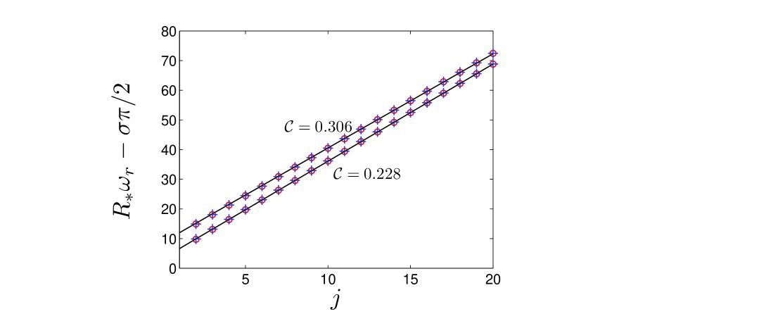
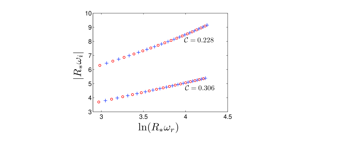
Figure 2: The axial (circles) and the polar (crosses) w-mode QNMs of two realistic stars obeying the analytic approximation of the SLy EOS proposed in Ref. Haensel and Potekhin (2004) with compactness ${\cal C}=0.306,\,0.228$ are shown. (a) $R_{*}\omega_{\rm r}-\sigma\pi/2$ is plotted against the mode number $j$, $j=1,2,...,20$. For clarity for the case ${\cal C}=0.306$ the data points are all shifted upward by 5. The two straight solid lines shown in the figure are the best linear fits to the two sets of data, respectively. (b) $|R_{*}\omega_{\rm i}|$ is plotted against $\ln(R_{*}\omega_{\rm r})$ for $5\leq j\leq 20$.

References

- Hughes (2003) S. Hughes, Ann. Phys. 303, 142 (2003).
- Abbott et al. (2009a) B. Abbott et al. (LIGO Scientific Collaboration), Phys. Rev. D. 80, 062001 (2009a).
- Abbott et al. (2009b) B. Abbott et al. (LIGO Scientific Collaboration), Phys. Rev. D. 80, 047101 (2009b).
- Abadie et al. (2010) J. Abadie et al. (LIGO Scientific Collaboration), Phys. Rev. D 82, 102001 (2010).
- Abbott et al. (2009c) B. Abbott et al. (LIGO Scientific Collaboration), Phys. Rev. D 79, 122001 (2009c).
- Belczynski et al. (2002) K. Belczynski, V. Kalogera, and T. Bulik, Astrophys. J. 572, 407 (2002).
- Lindblom et al. (1998) L. Lindblom, B. J. Owen, and S. M. Morsink, Phys. Rev. Lett. 80, 4843 (1998).
- Fryer et al. (2002) C. L. Fryer, D. E. Holz, and S. A. Hughes, Astrophys. J. 565, 430 (2002).
- Yamamoto et al. (2008) T. Yamamoto, M. Shibata, and K. Taniguchi, Phys. Rev. D 78, 064054 (2008).
- Dimmelmeier et al. (2008) H. Dimmelmeier, C. D. Ott, A. Marek, and H.-T. Janka, Phys. Rev. D 78, 064056 (2008).
- Baiotti et al. (2008) L. Baiotti, B. Giacomazzo, and L. Rezzolla, Phys. Rev. D 78, 084033 (2008).
- Duez et al. (2008) M. D. Duez, F. Foucart, L. E. Kidder, H. P. Pfeiffer, M. A. Scheel, and S. A. Teukolsky, Phys. Rev. D 78, 104015 (2008).
- Etienne et al. (2009) Z. B. Etienne, Y. T. Liu, S. L. Shapiro, and T. W. Baumgarte, Phys. Rev. D 79, 044024 (2009).
- Kiuchi et al. (2009) K. Kiuchi, Y. Sekiguchi, M. Shibata, and K. Taniguchi, Phys. Rev. D 80, 064037 (2009).
- Abdikamalov et al. (2009) E. B. Abdikamalov, H. Dimmelmeier, L. Rezzolla, and J. C. Miller, Mon. Not. R. Astron. Soc. 392, 52 (2009).
- Baiotti et al. (2009) L. Baiotti, S. Bernuzzi, G. Corvino, R. D. Pietri, and A. Nagar, Phys. Rev. D 79, 024002 (2009).
- Press (1971) W. Press, Astrophys. J. 170, L105 (1971).
- Leaver (1986) E. W. Leaver, Phys. Rev. D 34, 384 (1986).
- Ching et al. (1998) E. S. C. Ching, P. T. Leung, A. M. van den Brink, W. M. Suen, S. S. Tong, and K. Young, Rev. Mod. Phys. 70, 1545 (1998).
- Kokkotas and Schmidt (1999) K. D. Kokkotas and B. G. Schmidt, Living Rev. Rel. 2, 2 (1999).
- Berti et al. (2009) E. Berti, V. Cardoso, and A. O. Starinets, Class. Quant. Grav. 26, 163001 (2009).
- Andersson and Kokkotas (1996) N. Andersson and K. D. Kokkotas, Phys. Rev. Lett 77, 4134 (1996).
- Andersson and Kokkotas (1998) N. Andersson and K. D. Kokkotas, MNRAS 299, 1059 (1998).
- Benhar et al. (1999) O. Benhar, E. Berti, and V. Ferrari, MNRAS 310, 797 (1999).
- Kokkotas et al. (2001) K. D. Kokkotas, T. A. Apostolatos, and N. Andersson, MNRAS 320, 307 (2001).
- Benhar et al. (2004) O. Benhar, V. Ferrari, and L. Gualtieri, Phys. Rev. D 70, 124015 (2004).
- Tsui and Leung (2005) L. K. Tsui and P. T. Leung, Phys. Rev. Lett. 95, 151101 (2005).
- Tsui et al. (2006) L. K. Tsui, P. T. Leung, and J. Wu, Phys. Rev. D 74, 124025 (2006).
- Lau et al. (2010) H. K. Lau, P. T. Leung, and L. M. Lin, Astrophys. J. 714, 1234 (2010).
- Maggiore (2008) M. Maggiore, Phy. Rev. Lett. 100, 141301 (2008).
- Glendenning (1997) N. K. Glendenning, Compact Stars - Nuclear Physics, Particle Physics, and General Relativity (Springer, NY, 1997).
- Tolman (1939) R. C. Tolman, Phys. Rev. 55, 364 (1939).
- Oppenheimer and Volkoff (1939) J. R. Oppenheimer and G. M. Volkoff, Phys. Rev. 55, 374 (1939).
- Cox (1980) J. Cox, Theory of Stellar Pulsation (Princeton University Press, 1980).
- Regge and Wheeler (1957) T. Regge and J. A. Wheeler, Phys. Rev. 108, 1063 (1957).
- Chandrasekhar and Ferrari (1991a) S. Chandrasekhar and V. Ferrari, Proc. R. Soc. A 432, 247 (1991a).
- Thorne and Campolattaro (1967) K. S. Thorne and A. Campolattaro, Astrophys. J. 149, 591 (1967).
- Lindblom and Detweiler (1983) L. Lindblom and S. L. Detweiler, Astrophys. J. 53, 73 (1983).
- Detweiler and Lindblom (1985) S. Detweiler and L. Lindblom, Astrophys. J. 292, 12 (1985).
- Chandrasekhar and Ferrari (1991b) S. Chandrasekhar and V. Ferrari, Proc. R. Soc. A 433, 423 (1991b).
- Chandrasekhar and Ferrari (1991c) S. Chandrasekhar and V. Ferrari, Proc. R. Soc. A 434, 449 (1991c).
- Chandrasekhar and Ferrari (1995) S. Chandrasekhar and V. Ferrari, Proc. R. Soc. A 263, 450 (1995).
- Ipser and Price (1991) J. R. Ipser and R. H. Price, Phys. Rev. D 43, 1768 (1991).
- Allen et al. (1998) G. Allen, N. Andersson, K. D. Kokkotas, and B. F. Schutz, Phys. Rev. D 58, 124012 (1998).
- Lindblom et al. (1997) L. Lindblom, G. Mendell, and J. R. Ipser, Phys. Rev. D. 56, 2118 (1997).
- Andersson et al. (1996) N. Andersson, K. D. Kokkotas, and B. F. Schutz, MNRAS 280, 1230 (1996).
- Wu and Leung (2007) J. Wu and P. T. Leung, MNRAS 381, 151 (2007).
- Akmal et al. (1998) A. Akmal, V. R. Pandharipande, and D. G. Ravenhall, Phys. Rev. C 58, 1804 (1998).
- Zerilli (1970) F. J. Zerilli, Phys. Rev. Lett. 24, 737 (1970).
- Ching et al. (1995) E. S. C. Ching, P. T. Leung, W. M. Suen, and K. Young, Phys. Rev. Lett. 74, 4588 (1995).
- Ching et al. (1996) E. S. C. Ching, P. T. Leung, W. M. Suen, and K. Young, Phys. Rev. D 54, 3778 (1996).
- Berry (1982) M. V. Berry, J. Phys. A 15, 3693 (1982).
- Slavyanov (1996) S. Y. Slavyanov, Asymptotic Solutions of the One-Dimensional Schrödinger Equation (American Mathematical Society, USA, 1996).
- Zhang (2009) Y. J. Zhang, Master’s thesis, The Chinese University of Hong Kong (2009).
- Pandharipande (1971a) V. Pandharipande, Nucl. Phys A 174, 641 (1971a).
- Arnett and Bowers (1977) W. D. Arnett and R. L. Bowers, Astrophys. J. 33, 415 (1977).
- Pandharipande (1971b) V. Pandharipande, Nucl. Phys A 178, 123 (1971b).
- Wiringa et al. (1988) R. B. Wiringa, V. Fiks, and A. Fabrocini, Phys. Rev. C 38, 1010 (1988).
- Haensel and Potekhin (2004) P. Haensel and A. Y. Potekhin, Astron. Astrophy. 428, 191 (2004).
- Pandharipande and Ravenhall (1989) V. R. Pandharipande and D. G. Ravenhall, Proc. NATO Advanced Research Workshop on nuclear matter and heavy ion collisions, Les Houches, (Plenum, New York, 1989), p. 103.
- Douchin and Haensel (2001) F. Douchin and P. Haensel, Astron. Astrophys. 380, 151 (2001).
- Bleistein and Handelsman (1986) N. Bleistein and R. A. Handelsman, Asymptotic Expansion of Integrals (Dover, New York, 1986).
- Chandrasekhar (1983) S. Chandrasekhar, The Mathematical Theory of Black Holes (Oxford University Press, New York, 1983).
- Anderson and Price (1991) A. Anderson and R. Price, Phys. Rev. D 43, 3147 (1991).
- Leung et al. (2001) P. T. Leung, A. M. van den Brink, W. M. Suen, C. W. Wong, and K. Young, J. Math. Phys. 42, 4802 (2001).