Power-law tails in triple system decay statistics

Abstract

We have investigated the decay statistics of triple systems with different masses in Newtonian dynamics. We demonstrate that in a broad interval of mass ratios this statistics has good approximation by power-law tails. The power indices do not show any significant dependence on mass ratios.

I Introduction

Power-law tails in various branches of natural science have been intensively investigated during last several decades. These studies deal with experimental results on existing of power-law tails as well as attempts of theoretical explanation of this phenomenon. Some experimental material have been collected in a popular review (Schroeder, 1991), other examples important for astrophysics see, for example, in Alberico et al. (2000); Wilk & Wlodarczyk (2000). As an example of theoretical description it is possible to note a progress in modern statistical physics which predicts power-law tails by using non-classical definitions of entropy (this approach starts from works of Renyi (1970) and Tsallis (1988), for a modern review see, for example, Rudoi (2003)). For other approaches to possible source of this phenomenon see, for example, Montroll & Shlesinger (1983).

In hamiltonian dynamics power-law tails appear in two different situations: for systems with escape we can study the number of trajectories $N$ which survive up to time $t$ (or, alternatively, the number of trajectory $dN$ experienced the escape in the time interval from $t$ to $t+dt$ we will study this differential form of the time distribution of escapes in the present paper), for systems with a compact phase space it is possible to construct a function which describes Poincare recurrence time depending on the initial position in the phase space. Many empirical results show that the appearance of power-law tails in such systems is connected with islands of a regular motion in the phase space and “stickness” of trajectories to the boundaries of these islands (Zaslavsky, 2007), though strict mathematical results about this kind of systems are still rather poor.

Three-body problem is an example of combined dynamics – it is known that stable periodic orbits surrounded by islands of regular dynamics exist in a chaotic ”sea” representing the bulk of phase space. For equal-mass problem (when all three masses have the same value) there exists stable configuration called a “figure-eight” orbit (Chenciner & Montgomery, 2000), as well as several other orbits (Martynova et al., 2009). It is also known that the ”figure-eight” orbit becomes unstable when relative differenses in masses reach approximately $10^{-2}$ (Simo, 2000), so this very interesting orbit is hardly important for any real astrophysical problem. The Schubart orbit (Schubart, 1956) remaines stable in a much broader interval of masses (Orlov et al., 2008) On the other hand, famous triangle Lagrange points become stable in the situation of suffitiently different masses, and we can imagine that set of stable orbits have rather nontrivial dependence on mass differences.

The phenomenon of trajectory “stickness” to boundary of a regular region for the three-body problem has already been remarked by Dvorak et al. (1998) and Martynova et al. (2009). Keeping this in mind we can expect existence of power-law tails in $N(t)$ distribution. For other theoretical arguments supporting this suggestion see Agekian at al. (1983). Earlier attempts to describe this function have been done by Mikkola & Tanikawa (2007) where exponential ansatz for $N(t)$ have been used. However, Orlov et al. indicated that this modelling works only for a limited time interval, and for large enough time $t$ power-law tails become clearly detectable Orlov et al. (2010). Both these works deal with the equal-mass problem. This construction may be too symmetric for making general conclusions (keeping in mind loss of stability for ”figure-eight” solution” with a small mass inequality), so it is reasonable to provide similar analysis in a general situation with non-equal masses. In the present paper we have chosen several different mass ratios for investigation, starting from near-equal mass system and concluding for the system with masses $(0.1,1,10)$ mass units, which means that Schubart orbit is already unstable, and Lagrange triangle points are still unstable for this mass ratio.

II System and initial data

Figure 1: The layout of the initial conditions (coordinates). The $m_{1}$ body is always in the (0, 0) point, $x$-coordinate of $m_{2}$ is varying within certain range. As for $m_{3}$, its both coordinates are varying — see text for details.

In the present paper we cover wide range of mass ratios from equal-mass problem to near hierarchical system. We use Aarseth code (Aarseth & Zare, 1974) and start from zero-velocity initial conditions. Time variable is chosen so that $G=1$.

The layout of the initial conditions we used in our study is given in Fig. 1. The first body with mass $m_{1}$ is initially located in the (0, 0) point, the second body $m_{2}$ initially lies on the ($a$, 0) segment with $a\in(n+\delta,2n+\delta)$, where $n$ is a space scale and $\delta$ is some small separation introduced to avoid the situation when two bodies have totally coinciding initial coordinates. Finally, the third body $m_{3}$ initially lies within a square $(b,c)$ with $b\in(0,2n)$ and $c\in(0+\delta,2n+\delta)$. This choice cover rather wide area in the initial condition space for our results to be representent, on the other hand, different permutations of non-equal masses results in different initial condition sets allowing us to study possible dependence of our results upon initial conditions chosen.

Using the described above layout we evenly distribute about 4 millions initial configurations and calculate their evolution until the decay (for exact meaning of the decay in Aarseth code see, for example, Orlov et al. (2010)).

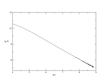
Figure 2: The typical plot of $N(t)$ in the logarithmic scale.

III Decay spectra

A typical plot of the differential distribution $N(t)$ in the logarithmic scale is shown in Fig. 2. Power-law tail following a steeper function after $t$ reaches the value of about one thousand is clearly seen. The distribution of escaping time for small $t$ is clearly different from power-law, and to obtain correct values of power index in the modelling

$$N(t)={\rm const}\times t^{-\gamma}$$

we should exclude this range of $t$ from the analysis. As an illustration we plot in Fig. 3 power indices calculated in the time range from $t_{in}$ to $T_{f}$ where the maximal time of integration $T_{f}=7000$. We can see that the power index typically does not change if $t_{in}$ is bigger than $2000$. In what follows we will ignore first $2000$ time units in calculation of power index $\gamma$. In the table below we present minimal and maximal values of $\gamma$ for several mass combinations calculated for different sets of initial conditions. Error bars, also presented in the table indicate that in some situations the difference in power indices calculated for the same system using different sets of initial conditions can be real (though not so big). We can see also that despite mass ratio of the systems under investigation cover a broad interval from near-equal to near-hierarchical systems, the value of $\gamma$ does not change significantly with the slightly developed tendency of growing $\gamma$ with the increasing hierarchicity of the triple system. We should, however, note that our values of $\gamma$ for equal mass system is bigger than the value found in the paper Orlov et al. (2010). Can different sets of initial conditions be the only cause of this difference remaines unclear and requires further investigations.

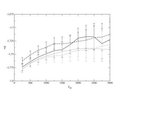
Figure 3: An examples of dependence of the slope $\gamma$ on the cutoff time $t_{in}$. Black lines corresponds to (1, 2, 3)_n=3 mass combination, grey – to (1, 3, 5)_n=5. Different line styles correspond to different distribution of masses between $m_{1}$, $m_{2}$ and $m_{3}$.

Table 1: Maximal and minimum values for the slope $\gamma$, calculated at $t_{in}=3000$ for different mass combinations. First column gives absolute masses, second – masses, normalized to $m_{1}+m_{2}+m_{3}=1$, third – the slope $\gamma$ with an error, minimal (upper row) and maximal (lower row) values.

Masses		$\gamma\pm\delta\gamma$
(0.1, 1, 10)	(0.009, 0.09, 0.901)	1.762	0.011
		1.863	0.016
(1, 3, 10)	(0.071, 0.214, 0.715)	1.845	0.013
		1.862	0.012
(1, 3, 5)	(0.111, 0.333, 0.556)	-1.828	0.013
		1.848	0.014
(1, 2, 3)	(0.167, 0.333, 0.5)	1.857	0.014
		1.905	0.015
(0.9, 1, 1.1)	(0.3, 1/3, 11/30)	2.149	0.009
		2.181	0.010
(1, 1, 1)	(1/3, 1/3, 1/3)	2.125	0.014
		2.178	0.012

IV Conclusions

We studied the escaping rate statistics in a general three-body problem with non-equal masses. We argue that for large enough time $t$ this statistics can be modelled by power-law functions with a good accuracy. For all cases studied (with normalized mass ratios from to) the power index is located within a rather narrow interval (from $1.76$ to $2.19$).

References

- Schroeder (1991) M. Schroeder, Fractals, Chaos, Power-laws, W.H.Freeman, NY (1991).
- Alberico et al. (2000) W.M. Alberico, A. Lavagno, and P.Quarati, Eur. Phys. J. C. 12, 499 (2000).
- Wilk & Wlodarczyk (2000) G. Wilk and Z. Wlodarczyk, Phys. Rev. Lett. 84, 2770 (2000).
- Renyi (1970) A.Renyi, Probabiliry Theory, Amsterdam: Noth-Holland (1970).
- Tsallis (1988) C. Tsallis, J. Stat. Phys., 52, 479 (1988).
- Rudoi (2003) Yu. Rudoi, Theoretical and Mathematical Physics, 135, 451 (2003).
- Montroll & Shlesinger (1983) E. Montroll and M. Shlesinger, J. Stat. Phys. 32, 209 (1983).
- Zaslavsky (2007) G. Zaslavsky, The Physics of Chaos in Hamiltonian Systems, London, Imperial College Press (2007).
- Chenciner & Montgomery (2000) A. Chenciner and R. Montgomery, Ann. Math. 52, 881 (2000).
- Martynova et al. (2009) A. Martynova, V. Orlov, and A. Rubinov, Astronomy Reports, 53, 710 (2009).
- Simo (2000) K. Simo, in: Celectial Mechanics, dedicated to Donald Saari for his 60th birthday, Northwesten University, Evanston, Illinois (2000).
- Schubart (1956) J. Schubart, Astronomische Nachriften, 283, 17 (1956).
- Orlov et al. (2008) V. Orlov, A. Petrova, K. Tanikawa, M. Saito, and A. Martynova, Cel. Mech. Dyn. Astr., 100, 93 (2008).
- Dvorak et al. (1998) R. Dvorak, G. Contopoulos, Ch. Efthymiopoulos, and N. Voglis, Planetary Space Sci., 46, 1567 (1998).
- Agekian at al. (1983) T. Agekian, Zh. Anosova, and V. Orlov, Astrophys., 19, 66 (1983).
- Mikkola & Tanikawa (2007) S. Mikkola and K. Tanikawa, Mon. Not. Roy. Astron. Soc., 379, L21 (2007).
- Orlov et al. (2010) V. Orlov, A. Rubinov, and I. Shevchenko, Mon. Not. Roy. Astron. Soc., 408, 1623 (2010).
- Aarseth & Zare (1974) S. Aarseth and Zare, Celestial Mechanics 10, 185 (1974).