Lattice QCD with Optimal Domain-Wall Fermion: Light Meson Spectroscopy

Abstract:

We perform lattice simulations of two flavors QCD using the optimal domain-wall fermion, in which the chiral symmetry is preserved to a good precision ($m_{res}\sim 0.3$ MeV) on the $16^{3}\times 32$ lattice ($L\sim 2$ fm) with inverse lattice spacing $a^{-1}\sim 1.8$ GeV, and $N_{s}=16$ in the fifth dimension, for eight sea quark masses corresponding to the pion masses in the range 210-500 MeV. We present our first results of the mass and the decay constant of the pseudoscalar meson, which are in good agreement with the next-to-leading order chiral perturbation theory for $M_{\pi}<450$ MeV, and from which we determine the low-energy constants $f$, $\Sigma$, $\bar{l}_{3}$ and $\bar{l}_{4}$. At the physical pion mass $M_{\pi}=135$ MeV, we obtain the pion decay constant $f_{\pi}=133(1)(2)$ MeV, and the average up and down quark mass $m_{ud}^{\overline{\rm MS}}(\mathrm{2~{}GeV})=4.09(7)(11)$ MeV, where the first error is statistical, and the second error is systematic due to the truncation of the higher order corrections and the uncertainty in the determination of the lattice spacing. Furthermore, we also obtain the chiral condensate $\Sigma^{\overline{{\mathrm{MS}}}}(\mbox{2~{}GeV})=[\mbox{250(4)(7)~{}MeV}]^{3}$.

1 Introduction

Lattice QCD with exact chiral symmetry is an ideal theoretical framework to study the nonperturbative physics from the first principles of QCD. However, it is rather nontrivial to perform Monte Carlo simulation such that the chiral symmetry is perserved to a very high precision and all topological sectors are sampled ergodically.

Since 2009, the Taiwan Lattice QCD Collaboration (TWQCD) has been using a GPU cluster (currently constituting of 250 NVIDIA GPUs) which attains 40 Teraflops (sustained) to simulate unquenched lattice QCD with the optimal domain-wall quarks [1, 2]. We have realized our goal of preserving the chiral symmetry to a good precision (with $m_{res}\sim 0.3$ MeV) and also sampling all topological sectors ergodically.

In this paper, we present our first results of the mass and the decay constant of the pseudoscalar meson in two flavors QCD, and compare our results with the next-to-leading order (NLO) chiral perturbation theory (ChPT). We find that our data is in good agreement with NLO ChPT for $M_{\pi}$ less than 450 MeV, and from which we determine the low-energy constants $f$, $\Sigma$, $\bar{l}_{3}$ and $\bar{l}_{4}$, and and the average up and down quark mass $m_{ud}^{\overline{\rm MS}}(\mathrm{2~{}GeV})$. Our result of the topological susceptibility is presented in Ref. [3], and our strategy of using GPU to speed up our Hybrid Monte Carlo simulations is presented in Ref. [4].

2 Hybrid Monte Carlo Simulation with Optimal Domain-Wall Quarks

The optimal domain-wall fermion is the theoretical framework which preserves the (mathematically) maximal chiral symmetry for any finite $N_{s}$ (the length of the fifth dimension). Thus the artifacts due to the chiral symmetry breaking with finite $N_{s}$ can be reduced to the minimum.

The action of the optimal domain-wall fermion is defined as [1]

$$S_{\mathrm{odwf}}=\sum_{s,s^{\prime}=1}^{N_{s}}\sum_{x,x^{\prime}}\bar{\psi}_{xs}\left[(\omega_{s}D_{w}+1)_{xx^{\prime}}\delta_{ss^{\prime}}+(\omega_{s}D_{w}-1)_{xx^{\prime}}L_{ss^{\prime}}\right]\psi_{x^{\prime}s^{\prime}}\equiv\bar{\Psi}\mathcal{D}\Psi,$$ (1)

where the weights $\{\omega_{s}\}$ along the fifth dimension are fixed according to the formula derived in Ref. [1] such that the maximal chiral symmetry is attained. Here $D_{w}$ denotes the standard Wilson-Dirac operator plus a negative parameter $-m_{0}\;(0<m_{0}<2)$,

$$(D_{w})_{xx^{\prime}}=-\frac{1}{2}\sum_{\mu}\left[(1-\gamma_{\mu})U_{\mu}(x)\delta_{x+\hat{\mu},x^{\prime}}+(1+\gamma_{\mu})U^{\dagger}_{\mu}(x^{\prime})\delta_{x-\hat{\mu},x^{\prime}}\right]+(4-m_{0}),$$ (2)

and

$$L=P_{+}L_{+}+P_{-}L_{-},\quad P_{\pm}=(1\pm\gamma_{5})/2,$$ (3)

$$(L_{+})_{ss^{\prime}}=\left\{\begin{array}[]{ll}\delta_{s-1,s^{\prime}},&1<s\leq N_{s}\\ -(m_{q}/2m_{0})\delta_{N_{s},s^{\prime}},&s=1\end{array}\right.;\quad\quad L_{-}=(L_{+})^{T},$$ (4)

where $m_{q}$ denotes the bare quark mass. Separating the even and the odd sites on the 4D space-time lattice, $\mathcal{D}$ can be written as

$$\mathcal{D}(m_{q})=S_{1}^{-1}\begin{pmatrix}1&M_{5}D_{w}^{\text{EO}}\\ M_{5}D_{w}^{\text{OE}}&1\end{pmatrix}S_{2}^{-1}=S_{1}^{-1}\begin{pmatrix}1&0\\ M_{5}D_{w}^{\text{OE}}&1\end{pmatrix}\begin{pmatrix}1&0\\ 0&C\end{pmatrix}\begin{pmatrix}1&M_{5}D_{w}^{\text{EO}}\\ 0&1\end{pmatrix}S_{2}^{-1},$$ (5)

where

$$M_{5}\equiv\left[(4-m_{0})+\sqrt{\omega}^{-1}(1-L)(1+L)^{-1}\sqrt{\omega}^{-1}\right]^{-1},\quad(\omega)_{ss^{\prime}}=\omega_{s}\delta_{ss^{\prime}},$$ (6)

$$S_{1}\equiv M_{5}\sqrt{\omega}^{-1},\quad S_{2}\equiv(1+L)^{-1}\sqrt{\omega}^{-1},$$ (7)

and the Schur decomposition has been used in the last equality of (5), with the Schur compliment

$$C=1-M_{5}D_{w}^{\text{OE}}M_{5}D_{w}^{\text{EO}}.$$ (8)

Since $\det\mathcal{D}=\det S_{1}^{-1}\cdot\det C\cdot\det S_{2}^{-1}$, and $S_{1}$ and $S_{2}$ do not depend on the gauge field, we can just use $C$ for the HMC simulation. After including the Pauli-Villars fields (with $m_{q}=2m_{0}$), the pseudo-fermion action for 2-flavor QCD ($m_{u}=m_{d}$) can be written as

$$S_{pf}=\phi^{\dagger}C_{PV}^{\dagger}(CC^{\dagger})^{-1}C_{PV}\phi,\quad C_{PV}\equiv C(2m_{0}).$$ (9)

In the HMC simulation, we first generate random noise vector $\xi$ with Gaussian distribution, then we obtain $\phi=C_{PV}^{-1}C\xi$ using the conjugate gradient (CG). With fixed $\phi$, the system is evolved with a fictituous Hamiltonian dynamics, the so-called molecular dynamics (MD). In the MD, we use the Omelyan integrator [5], and the Sexton-Weingarten multiple-time scale method [6]. The most time-consuming part in the MD is to compute the vector $\eta=(CC^{\dagger})^{-1}C_{PV}\phi$ with CG, which is required for the evaluation of the fermion force in the equation of motion of the conjugate momentum of the gauge field. Thus we program the GPU to compute $\eta$, using CG with mixed precision [4]. Also, we have ported the computation of the gauge force and the update of the gauge field to the GPU.

Furthermore, we introduce an extra heavy fermion field with mass $m_{H}$ ($m_{q}\ll m_{H}<2m_{0}$), similar to the case of the Wilson fermion [7]. For two flavors QCD, the pseudofermion action becomes

$$S_{pf}^{H}=\phi^{\dagger}C_{H}^{\dagger}\frac{1}{CC^{\dagger}}C_{H}\phi+\phi_{H}^{\dagger}C_{PV}^{\dagger}\frac{1}{C_{H}C_{H}^{\dagger}}C_{PV}\phi_{H},\quad C_{H}\equiv C(m_{H}),$$ (10)

which gives exactly the same fermion determinant of (9). However, the presence of the heavy fermion field plays the crucial role in reducing the light fermion force and its fluctuation, thus diminishes the change of the Hamiltonian in the MD trajactory, and enhances the acceptance rate.

For a system with CPU and GPU, we can have both of them compute concurrently, e.g., while the GPU is working on the CG of the light quark field, the CPU can compute the fermion force of the heavy fermion field. This asynchronous concurrent excecution mode enhances the overall performance by $\sim 5\%$.

A detailed description of our HMC simulations will be presented in a forthcoming paper [8].

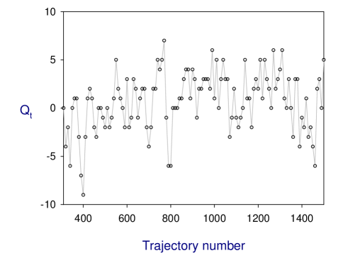
Figure 1: The topological charge versus the trajectory in the HMC simulation of two flavors QCD with ODWF. The lattice is $16^{3}\times 32$ with the spatial box $\sim(\mbox{2 fm})^{3}$, and the quark mass corresponding to $M_{\pi}\sim 300$ MeV. The topological charge is obtained by projecting the zero modes of the overlap Dirac operator.

3 Lattice setup

We simulate two flavors ($N_{f}=2$) QCD on the $16^{3}\times 32$ lattice at the lattice spacing $a\sim$ 0.11 fm, for eight sea quark masses in the range $m_{q}a=0.01,0.02,\cdots,0.08$. For the gluon part, we use the plaquette action at $\beta$ = 5.90. For the quark part, we use the optimal domain-wall fermion with $N_{s}=16$. After discarding 300 trajectories for thermalization, we accumulated about $3000-3200$ trajectories in total for each sea quark mass. From the saturation of the error (by binning) of the plaquette, as well as the evolution of the topological charge (see Fig. 1), we estimate the autocorrelation time to be $\sim 10$ trajectories. Thus we sample one configuration every 10 trajectories. Then we have $270-290$ configurations for each sea quark mass.

We determine the lattice spacing by heavy quark potential with Sommer parameter $r_{0}=0.49$ fm. The inverse lattice spacing versus the quark mass is plotted in Fig. 2. Using the linear fit, we obtain the inverse lattice spacing in the chiral limit, $a^{-1}=1.8153(28)$ GeV.

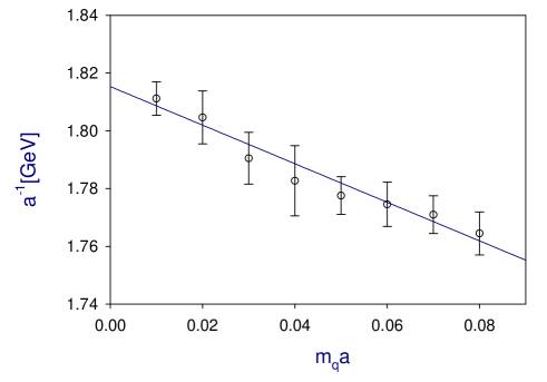
Figure 2: The inverse lattice spacing $a^{-1}$ [GeV] versus $m_{q}a$ for two flavors QCD with ODWF.

For each configuration, we calculate the exact zero modes plus 80 conjugate pairs of the lowest-lying eignmodes of the overlap Dirac operator. We outline our procedures as follows. First, we project 240 low-lying eigenmodes of $H_{w}^{2}$ using $\nu$-TRLan alogorithm [9], where each eigenmode has a residual less than $10^{-12}$. Then we approximate the sign function of the overlap operator by the Zolotarev optimal rational approximation with 64 poles, where the coefficents are fixed with $\lambda_{max}^{2}=(6.4)^{2}$, and $\lambda_{min}^{2}$ equal to the maximum of the 240 projected eigenvalues of $H_{w}^{2}$. Then the sign function error is less than $10^{-14}$. Using the 240 low-modes of $H_{w}^{2}$ and the Zolotarev approximation with 64 poles, we project the zero modes plus 80 conjugate pairs of the lowest-lying eignmodes of the overlap operator with the $\nu$-TRLan algorithm, where each eigenmode has a residual less than $10^{-12}$.

We measure the chiral symmetry breaking (due to finite $N_{s}$) by computing the residual mass

$$m_{res}\equiv\left<\frac{\sum_{x}\left<J_{5}(x,N_{s})\bar{q}(0)\gamma_{5}q(0)\right>}{\sum_{x}\left<\bar{q}(x)\gamma_{5}q(x)\bar{q}(0)\gamma_{5}q(0)\right>}\right>_{\{U\}}=\left<\frac{\mathrm{tr}(D_{c}+m_{q})^{-1}_{0,0}}{\mathrm{tr}[(D_{c}^{\dagger}+m_{q})(D_{c}+m_{q})]^{-1}_{0,0}}\right>_{\{U\}}-m_{q},$$ (11)

where $(D_{c}+m_{q})^{-1}$ is the valence quark propagator with $m_{q}$ equal to the mass of the sea quark, tr denotes the trace running over the color and Dirac indices, and the subscript $\{U\}$ denotes averaging over an ensemble of gauge configurations. It turns out that, after averaging over an ensemble of a few hundreds of independent gauge configurations, $m_{res}$ is insensitive to the location of the origin $x^{\mu}=(0,0,0,0)$. Thus (11) gives a reliable measure of chiral symmetry breaking due to finite $N_{s}$. The derivation of (11) will be given in a forthcoming paper [10].

In Fig. 3, we plot the residual mass versus the quark mass. Using the power-law fit, we obtain the residual mass in the chiral limit, $m_{res}a=0.00018(2)$, which amounts to $m_{res}=0.32(4)$ MeV. Note that the value of $m_{res}$ is less than 1/10 of the statistical and systematic errors of the inverse lattice spacing, thus confirming that the chiral symmetry has been preserved to a good precision in our simulation.

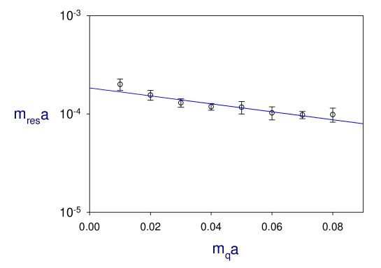
Figure 3: The residual mass versus the quark mass for two flavors QCD with ODWF.

4 The Mass and the Decay Constant of the Pseudoscalar Meson

In this section, we present our first results of the pseudoscalar mass and decay constant, for 2 flavors QCD with optimal domain-wall quarks and the plaquette gluon action at $\beta=5.90$, on the $16^{3}\times 32\times 16$ lattice. In Fig. 4, we plot $M_{\pi}^{2}/m_{q}$ and $f_{\pi}$ versus $m_{q}$ respectively. Here we have made the correction for the finite volume effect using the estimate within ChPT calculated up to ${\cal O}(M_{\pi}^{4}/(4\pi f_{\pi})^{2})$ [12], since our simulation is done on a finite volume lattice with $M_{\pi}L\sim 2.0$ for the lightest sea quark, and its finite volume effect cannot be neglected.

Taking into account of the correlation between $M_{\pi}^{2}/m_{q}$ and $f_{\pi}$ for the same sea quark mass, we fit our data to the formulas of the next-to-leading order (NLO) chiral perturbation theory (ChPT) [11]

$$\frac{M_{\pi}^{2}}{m_{q}} = 2B\left[1+\left(\frac{2Bm_{q}}{16\pi^{2}f^{2}}\right)\ln\left(\frac{2Bm_{q}}{\Lambda_{3}^{2}}\right)\right],\quad B\equiv\frac{2\Sigma}{f^{2}}$$ (12)

$$f_{\pi} = f\left[1-\left(\frac{4Bm_{q}}{16\pi^{2}f^{2}}\right)\ln\left(\frac{2Bm_{q}}{\Lambda_{4}^{2}}\right)\right],$$ (13)

where $\Lambda_{i}$ are related to the low energy constants $\bar{l}_{i}$

$$\bar{l}_{3}=\ln\left(\frac{\Lambda_{3}^{2}}{m_{\pi^{\pm}}^{2}}\right),\quad\bar{l}_{4}=\ln\left(\frac{\Lambda_{4}^{2}}{m_{\pi^{\pm}}^{2}}\right),\quad m_{\pi}^{\pm}=0.140\mbox{ GeV}.$$ (14)

For the six lightest quark masses (corresponding to pion masses in the range $210-445$ MeV), our fit gives

$$\Sigma=0.2105(30)\mbox{ GeV},\quad f=0.127(2)\mbox{ GeV},\quad\bar{l}_{3}=4.37(18),\quad\bar{l}_{4}=5.31(11),$$ (15)

with $\chi^{2}$/dof = 0.4. At the physical pion mass $M_{\pi}\simeq 0.135$ GeV, the value of pion decay constant is $f_{\pi}=0.133(1)$ GeV, and the bare quark mass is $0.0069(2)$ GeV. In order to convert the bare quark mass to that in the $\overline{\mathrm{MS}}$ scheme, we calculate the renormalization factor $Z_{m}^{\overline{\mathrm{MS}}}(\mathrm{2~{}GeV})$ using the non-perturbative renormalization technique through the RI/MOM scheme [13], and obtain $Z_{m}^{\overline{{\mathrm{MS}}}}(\mbox{2 GeV})=0.5934(10)$ [14]. Then the value of the average up and down quark mass is transcribed to

$$m_{ud}^{\overline{{\mathrm{MS}}}}(\mbox{2 GeV})=4.09(7)(11)\mbox{ MeV},$$ (16)

Similarly, the value of $\Sigma$ in (15) is transcribed to

$$\Sigma^{\overline{{\mathrm{MS}}}}(\mbox{2 GeV})=[250(4)(7)\mbox{ MeV}]^{3}$$ (17)

The systematic error is estimated from the turncation of higher order effects and the uncertainty in the determination of lattice spacing with $r_{0}=0.49$ fm. Since our calculation is done at a single lattice spacing, the discretization error cannot be quantified reliably, but we do not expect much larger error because our lattice action is free from $O(a)$ discretization effects.

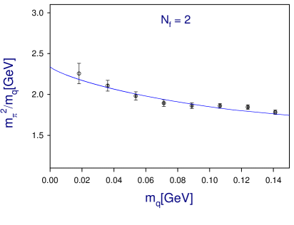
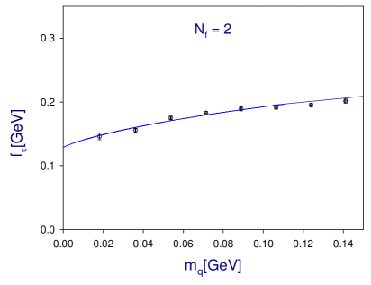
(a)	(b)

Figure 4: Physical results of 2-flavor QCD with optimal domain-wall quarks: (a) $m_{\pi}^{2}/m_{q}$, and (b) $f_{\pi}$. The solid lines are the simultaneous fits to the NLO ChPT, for the six lightest quark masses.

5 Concluding remarks

Using a GPU cluster (currently attaining 40 sustained Teraflops with 250 NVIDIA GPUs), we have succeeded to simulate unquenched lattice QCD with optimal domain-wall quarks, which preserves the chiral symmetry to a good precision and samples all topological sectors ergodically. Our results of the mass and the decay constant of the pseudoscalar meson (in this paper) and the topological susceptibility (in Ref. [3]) suggest that the nonperturbative chiral dynamics of the sea quarks are well under control in our simulations. This provides a new strategy to tackle QCD nonperturbatively from the first principles.

- [1] T. W. Chiu, Phys. Rev. Lett. 90, 071601 (2003); Nucl. Phys. Proc. Suppl. 129, 135 (2004)
- [2] T. W. Chiu et al. [TWQCD Collaboration], PoS LAT2009, 034 (2009) [arXiv:0911.5029 [hep-lat]].
- [3] T. H. Hsieh, T. W. Chiu, Y. Y. Mao [TWQCD Collaboration], PoS LAT2010, 085 (2010)
- [4] T. W. Chiu, T. H. Hsieh, Y. Y. Mao, K. Ogawa [TWQCD Collaboration], PoS LAT2010, 030 (2010)
- [5] T. Takaishi and P. de Forcrand, Phys. Rev. E 73, 036706 (2006)
- [6] J. C. Sexton and D. H. Weingarten, Nucl. Phys. B 380, 665 (1992).
- [7] M. Hasenbusch, Phys. Lett. B 519, 177 (2001)
- [8] T.W. Chiu et al. [TWQCD Collaboration], in preparation.
- [9] I. Yamazaki, Z. Bai, H. Simon, L.W. Wang, and K. Wu, Tech. Rep. LBNL-1059E (2008).
- [10] Y.C. Chen, T.W. Chiu [TWQCD Collaboration], in preparation.
- [11] J. Gasser and H. Leutwyler, Nucl. Phys. B 250, 465 (1985).
- [12] G. Colangelo, S. Durr and C. Haefeli, Nucl. Phys. B 721, 136 (2005)
- [13] G. Martinelli, C. Pittori, C. T. Sachrajda, M. Testa and A. Vladikas, Nucl. Phys. B 445, 81 (1995)
- [14] T.W. Chiu et al. [TWQCD Collaboration], in preparation.