Experimental determination of correlations between spontaneously formed vortices in a superconductor

Abstract

We have imaged spontaneously created arrays of vortices (magnetic flux quanta), generated in a superconducting film quenched through its transition temperature at rates around $10^{9}K/s$. From these images, we calculated the positional correlation functions for two vortices and for 3 vortices. We compared our results with simulations of the time dependent Ginzburg Landau equation in 2D. The results are in agreement with the Kibble-Zurek scenario of spontaneous vortex creation. In addition, the correlation functions are insensitive to the presence of a gauge field.

Vortices (magnetic flux quanta) are topological defects of the order parameter in a superconductor. These defects are predicted to appear spontaneously, as a result of a rapid quench through the phase transition into the superconducting state. During a rapid quench, close to the transition temperature ($T_{c}$), the relaxation time of the system becomes larger then the quench time. Under these conditions, the system is necessarily driven out of equilibrium. One model that describes the outcome of such phase transition is the Kibble-Zurek scenario, first suggested by KibbleKibble:1976 ; A.C. Davis and T.W.B. Kibble (2005) in a cosmological context. Among his other contributions, Zurek W.H. Zurek (1985) proposed terrestrial tests of this model in condensed matter systems, where the broken symmetry is U(1), such as superfluids, BEC and superconductors. The behavior of these systems can be described by a complex order parameter. Above the critical temperature $T_{c}$, the order parameter fluctuates with a characteristic size of the fluctuation being $\xi$. Is the sample is cooled infinitely slowly towards $T_{c}$, $\xi$ will grow until it reaches the size of the sample. At finite cooling rates the fluctuations ”freeze” at some point, forming isolated, uncorrelated domains of the ordered state. The typical size of such a domain, $\hat{\xi}$ , inside which the emerging order parameter is coherent, depends on the cooling rate. In equilibrium, the order parameter in the final state should be uniform across the system. However, the initial mismatch of the phase of the order parameter between different regions leads to the appearance of topological defects. In superconductors, these are vortices carrying a quantum of magnetic flux $\Phi_{0}\equiv h/2e$.

In the KZ model, below $T_{c}$ uncorrelated domains of the ordered state are formed. Each of these domains picks up a random value of phase of the order parameter. Single-valuedness of the order parameter requires that the integral of the phase accumulated along the circumference of any loop must be an integer multiple of $2\pi$. If the phases of different domains are random, there is a finite probability that the phase accumulated along a loop around a vertex between 3 domains will be $\pm 2\pi$, leading to formation of topological defect. To calculate the probability of this formation, the geodesic rule is usually implemented. It assumes that minimal phase gradient will always be favorable due to minimal energy consideration. Under this assumption, only one vortex can be created at a vertex between 3 ordered regions. Hence, the geodesic rule restricts the number of topological defects created by the system. This description is limited to relaxation of the phase gradients and does not involve any additional dynamics. One of the predictions of this model is strong, short range correlation between vortices and anti-vortices. If the size of frozen fluctuations $\hat{\xi}$ is assumed to have a gaussian distribution, one can calculate the vortex-vortex correlation function Liu:1992 . Hence, the fluctuations distribution above the critical temperature leaves its mark on the emerging vortex array. By measuring the positions of the vortices and calculating the correlation function it is possible to investigate the fluctuation distribution above $T_{c}$.

We note that the KZ model does not address the critical coarsening process which may occur after the transition Biroli:2010 . In many systems, coarsening affects drastically the outcome of the transition due to defect-antidefect annihilation. This may not be the case for superconducting films. If the quench is fast enough, the system reaches low temperatures before vortices can traverse the distance to a nearby antivortex and annihilate. At temperatures much lower than $T_{c}$ vortices are strongly pinned, so that any motion is practically impossible. As a result, vortex annihilation and coarsening is suppressed. Superconductors therefore offer us an unique opportunity to investigate the order parameter fluctuations above $T_{c}$, by measuring the vortex distribution after a quench.

The validity of KZ mechanism in systems with local gauge symmetries (such as superconductors), has been questioned by several authors Rudaz:1993 . For these systems an alternative mechanism of flux trapping was suggested Hindmarsh:2000 ; Kibble:2003 ; Donaire:2007 . In this mechanism thermal fluctuations of the magnetic field are frozen inside the superconductor during the transition. As a consequence vortices are formed in clusters of equal sign. The resulting vortex-vortex correlation function should decay as a power lawRajantie:2009 . However, the amplitude of trapped magnetic field fluctuations in conventional superconducting films should be so low that vortex formation should be better described by the Kibble Zurek mechanismDonaire:2007 .

It was suggested by several authors that topological defects in first order phase transitions Copeland:1996 ; Digal:1996a ; Digal:1996b ; Donaire:2009 and in sustems showing spinodal decomposition Pezzutti:2009 may form due to dynamics. In this approach, the geodesic rule does not hold anymore. Pairs of vortices and anti-vortices are formed during collisions between domain walls. Although most of the simulations were done for first order phase transitions, this mechanism is claimed to be generally applicable Digal:1997 . The correlation function for this mechanism was never calculated, but it should have two characteristic lengths: the separation between nearby vortices produced by domain wall collisions, and the domain size.

Vortex pairs of opposite sign could also arise from a Kosterlitz-Thouless type of transitionChu:2001 . In this theory, unbound vortex pairs appear above $T_{KT}$. If the system is cooled through $T_{KT}$, these vortices effectively annihilate. However, if the quench is fast, some of the unbound vortex pairs can survive the quench, become pinned at low temperatures and observed. In this theory, the density of unbound vortex pairs above $T_{KT}$ increases. Consequently, the observed vortex density should depend on the temperature from which the system is quenched. Within our resolution, we found no such dependence in the experiment described here.

The Kibble-Zurek (KZ) model has been tested in liquid helium Bauerle:1996 ; Ruutu:1996 , liquid crystals Rajarshi:2004 , in superconductors Maniv:2003 , Josephson junctions Carmi:2000 ; Monaco:2002 and superconducting loopsKirtley:2003 ; Monaco:2009 . Spontaneously generated topological defects were detected in several of the aforementioned experiments. More sensitive testing of the model involves the determination of correlations between these defects. There are only two such experiments performed to date. In one experimentRajarshi:2004 , done with liquid crystals, an array of topological defects was imaged. However, the amount of data was insufficient to detect correlations beyond nearest neighbors. In our experimentGolubchik:2010 , we imaged spontaneously formed arrays of vortices in a superconductor. The amount of data gathered was large, allowing a precise determination of the two point correlations. In this work, we extend this study to look at correlations between 3 defects.

Our experimental technique is described in detail in previous publicationsGolubchik:2009 ; Golubchik:2010 . Briefly, we image the magnetic field on the surface of a superconducting film using high resolution Magneto-optics. The superconductor sample consists of a $200nm$ thick Niobium film with $T_{c}$ of $8.9K$. The film is patterned into small squares of $200\mu m$ across. On top of the Nb film, we deposited a $40nm$ layer of $EuSe$ which serves as the Magneto-Optic sensor. To minimize the effect of stray magnetic fields, our apparatus was carefully shielded using $\mu$-metal. The residual field was less than $10^{-7}T$).

From our previous experiments Maniv:2003 , we know that extremely high cooling rates are essential for spontaneous generation of a measurable amount of vortices. No less important, fast cooling to low temperatures (far below $T_{c}$) traps the vortices on pinning centers, preventing annihilation of vortices and anti-vortices. Using short laser pulsesGolubchik:2010 , we achieved cooling rates as high as $2\cdot 10^{9}K/s$.

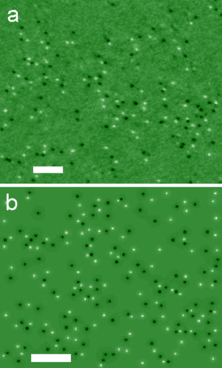
Figure 1: Spontaneously created vortices in a superconductor. a) A typical image of magnetic field created after a quench. The intensity is proportional to the local magnetic field. Bright and dark spots are vortices and anti-vortices respectively. The scale bar represents 10 $\mu m$. b) A typical result of the simulation of TDGL equations. The scale bar represents 10 $\xi_{0}$.

Fig.1a shows a typical image of spontaneously generated vortices. The average asymmetry between the density of positive and negative vortices is less than $1\%$. The average density of vortices was $6\cdot 10^{5}cm^{-2}$ for a cooling rate of $4\cdot 10^{8}K/s$ and $1.3\cdot 10^{6}cm^{-2}$ for a cooling rate of $2\cdot 10^{9}K/s$. The scaling of the density with the cooling rate is consistent with the KZ model at 2D (proportional to the square root of the cooling rate).

Our experimental results are compared with numerical simulations of the 2D time dependent Ginzburg-Landau equations. The simulations are described in detail in Ghinovker:2001 . Briefly, we used a square $200\times 200$ grid, with the parameters $\kappa=1$, $\Gamma=1$. The initial conditions, $A=0,\Psi=0,\theta=0.7$, mimic a quench from temperatures far above $T_{c}$ to $T=0.7T_{c}$. The implicit Crank-Nicholson scheme was employed on a staggered grid with step in time $\Delta\tau=0.01$ and in space $\Delta_{l}=0.2$. The time of each run was $20\tau_{GL}$. After this time the vortices are well defined and assumed to be pinned. A typical result is presented in fig.1b. Bright and dark spots mark the positions of vortices and anti-vortices. Several of the parameters of the simulation are different from the experimental parameters. First, the cooling rate in the simulation is infinite, in contrast to the finite rate in the experiment. Finite cooling rates in the simulation scale the correlation length but do not affect the distribution. Second, the simulation is fully two dimensional, while the sample used in the experiment is a thin film. The interaction between vortices in thin films is much stronger, and mediated through the magnetic field of the vortex outside of the film Brandt:2009 .

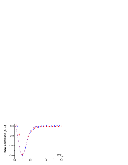
Figure 2: The vortex-vortex correlation function $G(r)$. Solid red triangles represent the correlation function calculated from experimental data. The statistical error bars are smaller than the point size. Open blue diamonds represent correlations calculated from the results of simulation. The solid line is a fit to theory of Liu and MazenkoLiu:1992 . The negative peak at short distance reflects vortex-antivortex correlations predicted by KZ model.

We used images like those shown in Fig.1 to determine the correlations between the vortices. The two particle vortex-vortex correlation function is defined as $G(r-r^{\prime})=<n(r)n(r^{\prime})>$ , with $n(r)=1$ at the location of a positive vortex, $-1$ at the location of negative vortex and $0$ elsewhere. The correlation function calculated from our data is shown in Fig.2. The distance in the figure was scaled by the mean vortex separation, $r_{av}=<\rho>^{-1/2}$ as proposed by Rajarshi:2004 . $r_{av}$ is related to $\hat{\xi}$ by $r_{av}=\frac{\hat{\xi}}{\sqrt{p}}$, where $p$ is the average number of vortices per domain. For our high cooling rate of $2\cdot 10^{9}K/s$, $r_{av}$ is $8.2\mu m$. The correlation function was averaged over 260 images, with 50,000 vortices in total. At the distance corresponding to the nearest neighbors the correlation function has a minimum. This is consistent with the KZ model which predicts that nearest neighbor vortices should have opposite polarities. The correlation function calculated from the simulations in the Fig.2 was averaged over 200 realizations. Since the same scaling was used, the experimental and simulated correlation functions can be compared without additional parameters. The dashed line is a fit to the theoretical predictions by Liu and MazenkoLiu:1992 with $\hat{\xi}=0.35r_{av}$. In their work, Liu and Mazenko assumed a Gaussian distribution of the fluctuations. Even through the simulation parameters differ from our experimental conditions (infinite vs. finite cooling rate, different initial temperatures, different interactions between vortices), the resulting correlation function is the same. Qualitatively similar correlation function was also calculated from simulations of quenched 2D XY modelJelic:2010 . The agreement with the correlation function calculated by Liu and MazenkoLiu:1992 suggests that in all cases, the shape of the correlation function is dictated by Gaussian fluctuations.

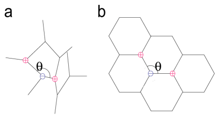
Figure 3: Schematic description of spontaneous formation of vortices on intersections between ordered domains. a) Random domain array. b) Close packed domain structure. Vortices and anti-vortices are marked by + and - respectively.

In addition to the two point correlation function $G(r-r^{\prime})$, we used our data to calculate an angular ( 3 point) correlation function. This function involves 3 vortices. For each vortex in the array, we look for its two nearest neighbors. Nearest neighbors are defined as vortices located within a distance of $\sim\hat{\xi}$ and have an opposite polarity (see fig.3). If such neighbors are found, we calculate the angle between the two lines connecting the vortex to its neighbors. In the limit where the domains are mono-dispersed and close packed (fig.3b), the angle between nearest neighbors will be $120^{o}$. For randomly distributed domains (fig.3a) the angles will have a broad distribution. Even through the connection between the fluctuation distribution and the angle distribution was never calculated, the first obviously determines the second. Therefore the comparison between the angle distribution calculated out of experimental data, and from the results of a simulation can be used as a validity test for a model. The angle distributions calculated from experimental data and from simulation are shown in Fig. 4. Both distributions have a minimum at $\theta=0^{o}$ and increase until $\theta\approx 100^{o}$ were they reach a plateau. Within the error bars, these two distributions are consistent.

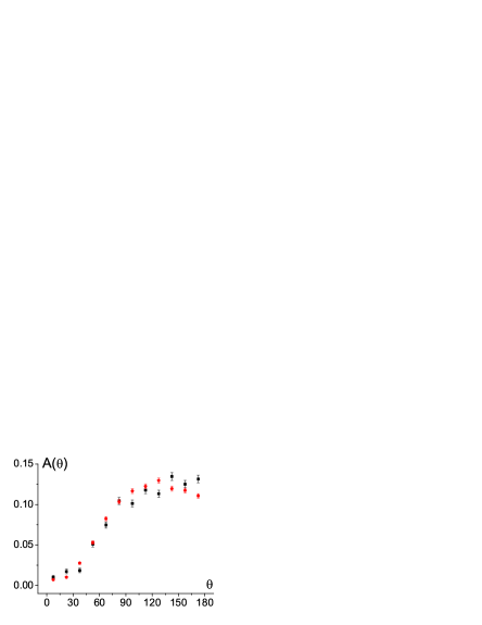
Figure 4: The angular distribution function. Solid black squares represent the angular distribution calculated from experimental data. Red pentagons are angular distribution calculated from the results of the simulation.

In conclusion, we calculated the vortex-vortex correlation function and the angular distribution function using experimental data and compared them with the results of TDGL simulations. We found an agreement between the experimental and simulated results. This implies that within experimental accuracy, the TDGL equation in 2D describes the vortex formation in our system. One consequence is that the coupling to the gauge field outside the sample does not affect the vortex distribution, at least for the parameters used in the experiment. The correlation function calculated using a quenched XY modelJelic:2010 gave qualitatively similar results, which suggests that gauge fields have no effect on the system evolution during quench.

- (1) T.W.B. Kibble J. Phys. A 9,1387, (1976)
- A.C. Davis and T.W.B. Kibble (2005) A.C. Davis, and T.W.B. Kibble Contemporary Physics 46, 313, (2005)
- W.H. Zurek (1985) W.H. Zurek Nature 317, 505, (1985)
- (4) F. Liu, and G. F. Mazenko Phys. Rev. B46, 5963, (1992)
- (5) G. Biroli, L. F. Cugliandolo, and A. Sicilia Phys. Rev. E81, 050101, (2010)
- (6) S. Rudaz and A. M. Srivastava, Mod. Phys. Lett. A 8, 1443 (1993); M. Hindmarsh, A. Davis and R. Brandenberger, Phys. Rev. D 49, 1944 (1994); T.W. B. Kibble and A. Vilenkin, Phys. Rev. D 52, 679 (1995).
- (7) M. Hindmarsh and A. Rajantie, Phys. Rev. Lett. 85, 4660 (2000)
- (8) T.W.B. Kibble and A. Rajantie, Phys. Rev. B68, 174512 (2003)
- (9) M. Donaire, T. W. B. Kibble and A. Rajantie, New Journal of Physics 9, 148, (2007)
- (10) A. Rajantie Phys. Rev. D79, 043515, (2009)
- (11) E.J. Copeland, and P.M. Saffin Phys. Rev. D54, 6088, (1996).
- (12) S. Digal, S. Sengupta, and A. Srivastava Phys. Rev. D58, 103510, (1996).
- (13) S. Digal, and A. Srivastava Phys. Rev. Lett. 76, 583, (1996).
- (14) M. Donaire, J. Phys. A 39, 15013 (2009).
- (15) A.D. Pezzutti, L.R. Gomez, M.A. Villar, and D.A. Vega Europhys. Lett., 87, 66003, (2009)
- (16) S. Digal, S. Sengupta, and A. Srivastava Phys. Rev. D55, 3824, (1997).
- (17) H.C. Chu, and G.A. Williams Phys. Rev. Lett. 86, 2585 (2001)
- (18) C. Bauerle, Y.M. Bunkov, C.N. Fisher, H. Godfrin, and G.R. Pickett, Nature 382, 332, (1996)
- (19) V.M.H. Ruutu, V.B. Eltsov, A.J. Gill, T.W.B. Kibble, M. Krusius, Yu.G. Marhlin, B. Plaçais, G.E. Volovik, and Wen Xu, Nature 382, 334, (1996).
- (20) R. Rajarshi, and A. Srivastava Phys. Rev. D69, 103525, (2004)
- (21) A. Maniv, E. Polturak, and G. Koren Phys. Rev. Lett. 91, 197001, (2003)
- (22) R. Monaco, J. Mygind, and R.J.Rivers Phys. Rev. Lett. 89, 080603, (2002)
- (23) R. Carmi, E. Polturak, and G. Koren Phys. Rev. Lett. , 84, 4966, (2000)
- (24) J.R. Kirtley, C.C.Tsuei, and F. Tafuri Phys. Rev. Lett. 90, 257001, (2003)
- (25) J.R. Monaco, J. Mygind, R.J. Rivers, and V.P. Koshelets Phys. Rev. B80, 180501, (2009)
- (26) D. Golubchik, G. Koren, and E. Polturak Phys. Rev. Lett. 104, 247002, (2010)
- (27) D. Golubchik, G. Koren, E. Polturak, and S. Lipson Optics Express, 17, 16160, (2009)
- (28) M. Ghinovker, B.Ya. Shapiro and I. Shapiro, Europhys. Lett., 53, 240 (2001)
- (29) E.H. Brandt Phys. Rev. B79, 134526, (2009).
- (30) A. Jelić, and L.F. Cugliandolo arXiv:1012.0417v1 (2010).