Localization and delocalization of two-dimensional discrete solitons pinned to linear and nonlinear defects

Abstract

We study the dynamics of two-dimensional (2D) localized modes in the nonlinear lattice described by the discrete nonlinear Schrödinger (DNLS) equation, including a local linear or nonlinear defect. Discrete solitons pinned to the defects are investigated by means of the numerical continuation from the anti-continuum limit and also using the variational approximation (VA), which features a good agreement for strongly localized modes. The models with the time-modulated strengths of the linear or nonlinear defect are considered too. In that case, one can temporarily shift the critical norm, below which localized 2D modes cannot exists, to a level above the norm of the given soliton, which triggers the irreversible delocalization transition.

I Introduction

The discrete nonlinear Schrödinger (DNLS) equations constitute a universal class of models which are profoundly interesting in their own right, as dynamical systems, and serve as models of a number of physical systems in nonlinear optics PhysRep , studies of Bose-Einstein condensates Smerzi ; morsch , and in other contexts Panos . In particular, soliton solutions to the DNLS equation in one, two, and three dimensions represent fundamental dynamically localized modes in discrete media. Experimentally, one- and two-dimensional (1D and 2D) discrete solitons have been created in nonlinear optical systems of several types PhysRep .

An important ingredient of DNLS models is represented by local defects. They are interesting as additional elements of the lattices Panos , and find important physical realizations. In particular, they may describe various strongly localized structures in photonic crystals defect0 , including nanocavities defect1 , as well as micro-resonators defect2 , and quantum dots defect3 .

The objective of the present work is to consider the interaction of 2D discrete solitons with local linear and nonlinear defects in DNLS lattices. The defect may be concentrated at a single site of the lattice, or it may be shaped as a Gaussian of a finite width. After introducing the model in Section 2, we consider stationary solitons pinned by the defects in Section 3. The analysis is performed by means of the variational approximation (VA) and numerical methods. In particular, the pinned-soliton families feature a specific combination of stable and unstable parts. In Section 4, we consider possibilities of the application of the “management” book to 2D discrete solitons, using the linear and nonlinear defects whose amplitudes slowly vary in time. In this direction, we analyze a possibility to trigger a delocalization transition by means of this method, which may be used in the design of switching schemes in photonics. Previously, the induced transition to the delocalization was demonstrates in uniform lattices with the inter-site coupling strength subject to the time modulation Bishop . The paper is concluded by Section 5.

II The model

We consider the following model based on the 2D DNLS equation with a local defect:

$$i\dot{u}_{n,m} + J\Delta_{2}u_{n,m}+V_{n,m}u_{n,m}$$ (1)

$$+ (\sigma+W_{n,m})|u_{n,m}|^{2}u_{n,m}=0,$$

where the overdot stands for the time derivative, $\Delta_{2}u_{n,m}\equiv u_{n,m+1}+u_{n,m-1}+u_{n+1,m}+u_{n-1,m}-4u_{n,m}$ is the 2D discrete Laplacian, the coupling constant of the lattice will be fixed by scaling, $J\equiv 1$, unless another choice of $J$ is specified explicitly, and $\sigma=+1$ and $-1$ corresponds to the attractive and repulsive nonlinearities, respectively ($\sigma=0$ for the linear lattice). Further, functions $V_{n,m}$ and $W_{n,m}$, which account for the linear and nonlinear components of the defect, are taken as Gaussians profiles,

$$V_{n,m} = v\exp\left[-(n^{2}+m^{2})/\Delta_{v}\right],$$

$$W_{n,m} = w\exp\left[-(n^{2}+m^{2})/\Delta_{w}\right],$$ (2)

with respective strengths $v,w$ and widths $\Delta_{v},\Delta_{w}$. In this notation, positive and negative strengths correspond to the attractive and repulsive defect, respectively. In fact, we will consider the linear and nonlinear defects separately. Models of 2D nonlinear lattices with other types of local defects were considered earlier Gaididei , including defects induced by edges of the lattice Kivshar .

Looking for the stationary solutions,

$$u_{n,m}=U_{n,m}\exp(-i\omega t),$$ (3)

we arrive at the nonlinear eigenvalue problem,

$$\omega U_{n,m} + \Delta_{2}U_{n,m}+V_{n,m}U_{n,m}$$ (4)

$$+ (\sigma+W_{n,m})|U_{n,m}|^{2}U_{n,m}=0,$$

for real frequency $\omega$ and the profile of the stationary discrete mode $U_{m,n}$, which may be complex, in the general case. In the absence of the defect, Eq. (4) gives rise to the linear dispersion relation featuring the phonon band, above and below which one can find nonlinear modes, described by respective curves $N(\omega)$, with $N=\sum_{m,n}|u_{m,n}|^{2}$ being the norm (power) of the nonlinear state. The important difference between 2D and 1D settings is that, in the latter case, the fundamental single-peak mode (the discrete soliton of the Sievers-Takeno type) persists in the limit of $N\rightarrow 0$, while all the 2D solitons are bounded by a critical norm, $N_{\mathrm{cr}}$, below which localized modes do not exist Panos . Accordingly, an abrupt delocalization (decay) of discrete 2D solitons was predicted in the case when the inter-site coupling constant would exceed a certain critical value Bishop . In the following we show that, introducing the defect with the linear and nonlinear components and varying their strengths, or the lattice coupling constant, one can change the critical norm, $N_{\mathrm{cr}}$, and thus control the transition to the delocalization.

III Stationary discrete solitons pinned to the defect: The variational approach and numerical results

III.1 The variational approximation

The variational approach (VA) was successfully used for the study of 2D discrete solitons in uniform (defect-free) DNLS lattices Weinstein ; CQ . Here, we start with the application of the VA to the 2D lattice in the presence of the $\delta$-defect localized at the origin:

$$i\dot{u}_{m,n}+\Delta_{2}u_{m,n}+\sigma|u_{m,n}|^{2}u_{m,n}$$

$$+(v+w|u_{m,n}|^{2})\delta_{m,0}\delta_{n,0}u_{m,n}=0,$$ (5)

cf. the more general form of the defect in Eq. (2). Generally, the strength of the defect may be time-dependent, $v=v(t),~{}w=w(t)$.

Equation (5) can be derived from the Lagrangian,

$$L = \frac{i}{2}\sum_{m,n}\left(u_{m,n}^{\ast}\dot{u}_{m,n}-u_{m,n}\dot{u}_{m,n}^{\ast}\right)$$ (6)

$$+ \sum_{m,n}\left[u_{m,n}^{\ast}\left(u_{m+1,n}+u_{m,n+1}\right)\right.$$

$$+ \left.u_{m,n}\left(u_{m+1,n}^{\ast}+u_{m,n+1}^{\ast}\right)-4|u_{m,n}|^{2}\right]$$

$$+ \frac{\sigma}{2}\sum_{m,n}|u_{m,n}|^{4}+v|u_{0,0}|^{2}+\frac{1}{2}w|u_{0,0}|^{4}.$$

To apply the VA, we adopt the following ansatz (previously, it was used for the analysis of discrete solitons in the 2D DNLS equation with the cubic-quintic nonlinearity CQ ):

$$u_{m,n}=\left\{\begin{array}[]{ll}B,&\mbox{if}\quad m=n=0;\\ Ae^{-a(|m|+|n|)},&\mbox{otherwise}.\end{array}\right.$$ (7)

Substituting ansatz (7) into Lagrangian (6), one can perform the respective calculations and find the effective Lagrangian as a sum of four terms which depend on three dynamical parameters, $(A,B,a)$ (which may be functions of time) and represent, respectively, the kinetic part, on-site self-interaction, inter-site couplings, and effects induced by the defect:

$$L=L_{\mathrm{kin}}+L_{\mathrm{coupl}}+L_{\mathrm{int}}+L_{\mathrm{self}}~{};$$ (8)

$$L_{\mathrm{kin}}=\frac{2ie^{-2a}}{\left(1-e^{-2a}\right)^{2}}\left(A^{\ast}\dot{A}-A\dot{A}^{\ast}\right)+\frac{i}{2}\left(B^{\ast}\dot{B}-B\dot{B}^{\ast}\right),$$ (9)

$$L_{\mathrm{self}}=2\sigma|A|^{4}\frac{e^{-4a}}{\left(1-e^{-4a}\right)^{2}}+\frac{\sigma}{2}|B|^{4},$$ (10)

$$L_{\mathrm{coupl}}=8|A|^{2}\frac{e^{-2a}}{\left(1-e^{-2a}\right)^{2}}\left(3e^{-a}-e^{-3a}-2\right)$$ (11)

$$+4(AB^{\ast}+A^{\ast}B)e^{-a}-4|B|^{2},$$ (12)

$$L_{\mathrm{defect}}=v|B|^{2}+\frac{w}{2}|B|^{4}~{}.$$ (13)

The substitution of the harmonic time dependence, $A(t)=Ae^{-i\omega t},~{}B(t)=Be^{-i\omega t},$ where $A$ and $B$ are real amplitudes, casts the Lagrangian into the following stationary form, with $C\equiv e^{-a}$:

$$L_{\mathrm{kin}}=4\omega\frac{A^{2}C^{2}}{\left(1-C^{2}\right)^{2}}+\omega B^{2},$$ (14)

$$L_{\mathrm{self}}=2\sigma A^{4}\frac{C^{4}}{\left(1-C^{4}\right)^{2}}+\frac{\sigma}{2}B^{4},$$ (15)

$$L_{\mathrm{coupl}}=8A^{2}\frac{C^{2}}{\left(1-C^{2}\right)^{2}}\left(3C-C^{3}-2\right)$$ (16)

$$+8ABC-4B^{2},$$ (17)

$$L_{\mathrm{defect}}=vB^{2}+\frac{w}{2}B^{4}~{}.$$ (18)

Fixing frequency $\omega$ and numerically solving the ensuing system of the Euler-Lagrange equations, which follows from the effective Lagrangian, $\partial L/\partial A=\partial L/\partial B=\partial L/\partial C=0,$ one can find the set of variational parameters $(A,B,a)$ and the norm corresponding to ansatz (7),

$$N=B^{2}\delta_{m,0}\delta_{n,0}+A^{2}\sum_{m,n}(1-\delta_{m,0}\delta_{n,0})C^{2(|m|+|n|)}~{}.$$ (19)

III.2 The linear defect

Curves $N(\omega)$ for the discrete solitons produced by the VA, along with their counterparts, obtained by dint of the direct numerical solution based on the continuation from the anti-continuum limit (see Appendix A), are displayed in Fig. 1, for the pure linear defect.

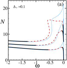
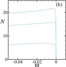
Figure 1: (Color online) (a) Comparison of the dependence of the norm on the frequency for the fundamental discrete solitons, as predicted by the VA, with the use of Eq. (19) (dotted blue lines), and its counterpart produced by the numerical solution of the stationary version of Eq. (5) (solid black and dashed red lines), for three different strengths of the linear defect ($w=0$): $v=-1;0;+1$ (from top to bottom; recall that $v>0$ and $v<0$ correspond to the attractive and repulsive defects, respectively). The numerical results were obtained for a narrow defect, with width $\Delta_{v}=0.1$ in Eq. (2). The nonlinearity is attractive ($\sigma=+1$). (b) Zoom of the plot in (a), corresponding to the VA prediction for the norm given by Eq. (19), in the vicinity of $\omega=0$. In this and all other figures, solid and dashed portions of the numerically generated curves depict subfamilies of stable and unstable solitons, respectively.

Figure 1(a) shows that, in the case of $\Delta_{v}=0.1$, which is practically tantamount to the defect localized at the single site, cf. Eq. (5), the VA-generated norm is in a good agreement with with the numerical results far from the limit of $\omega\rightarrow 0$. At small $\omega$, the soliton spreads out, and its actual shape deviates from the exponential ansatz (7), which leads to a discrepancy between the variational and numerical results, as seen in Fig. 1(a). Also due to restrictions on the size of the domain of calculation (in our case we used $41\times 41$ grid points) the numerical curves cannot be continued to extremely small values of $\omega$, therefore they are not presented in Fig. 1(b).

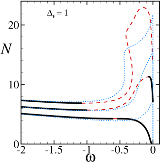
Figure 2: (Color online) The same as in Fig. 1(a), but with the norm found numerically for the broad defect with width $\Delta_{v}=1$.

Naturally, the increase of the width of the defect to $\Delta_{v}=1$, which makes the shape of defect (2) essentially different from that in Eq. (5), leads to a stronger discrepancy in the limit $\omega\rightarrow 0$, as seen in Fig. 2.

We have checked the linear stability of the solutions along their existence curves (see details in Appendix B). The results are shown by means of solid and dashed portions in the figures displaying the respective numerically generated $N(\omega)$ curves. Note that, here and in similar plots displayed below, the soliton families may contain two distinct stability segments separated by an instability region. It should be noted found that, far from the limit of $\omega=0$, the Vakhitov-Kolokolov (VK) criterion, $dN/d\omega<0$ Panos , correctly predicts the transition from the stability to instability at points where $dN/d\omega$ changes its sign from negative to positive. However, at small $\omega$, the formally applied VK criterion only partially complies with the linear-stability results, which may be an effect of boundary conditions on properties of very broad modes corresponding to small $\omega$.

It is worthy to note that, as one can conclude from the comparison of Figs. 1(a) and 2, the increase of the width of the attractive linear defect leads to a significant reduction of the instability region. This trend is also corroborated by the VK criterion.

III.3 The nonlinear defect

Similar results were obtained for the pure nonlinear defect, i.e., with $v=0$ in Eqs. (2) and (5), as shown in Figs. 3 and 4. In particular, analyzing the results for the linear and nonlinear defects with different widths, we have found that there is a particular intermediate value of the width in the interval of $\Delta_{v,w}\subset\left(0.1,1\right)$, at which the discrepancy between the numerical and variational solutions attains a minimum (in particular, it is $\Delta_{w}\approx 0.7$ for the nonlinear defect, see Fig.5).

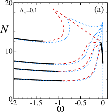
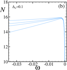
Figure 3: (Color online) The same as in Fig. 1, but for the pure nonlinear defect ($v=0$), at different values of its strength: $w=-0.5;-0.2;0;+0.5$ (from top to bottom). The width of the defect corresponding to the numerical curves is $\Delta_{w}=0.1$.

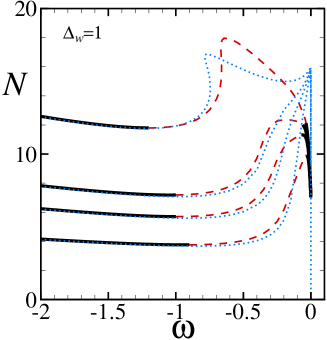
Figure 4: (Color online) The same as in Fig. 3(a), but for the defect’s width $\Delta_{w}=1$.

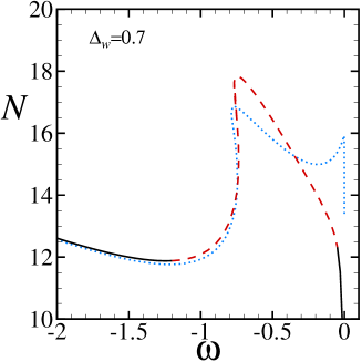
Figure 5: (Color online) The comparison between the variational and numerical results for the pure nonlinear defect with amplitude $w=-0.5$ and width $\Delta_{w}=0.7$. In this case, the overall discrepancy between the VA-predicted and numerically found curves [which are defined as in Fig. 3(a)] attains its minimum.

For the sake of comparison, the VA-predicted and numerical curves $N(\omega)$ are also shown in Fig. 6 for the discrete solitons in the defect-free 2D lattice (of course, these results are not different from those reported in earlier works which were dealing with the 2D DNLS equation without defects Weinstein ; Panos ). Comparing these to Figs. 1 and 3, we conclude that the discrepancy between the VA and numerical findings is actually smaller in the presence of the linear or nonlinear defect.

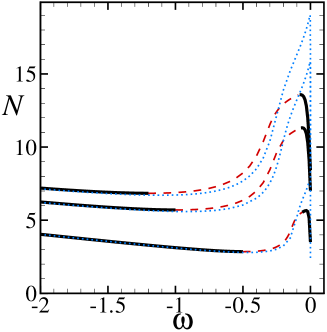
Figure 6: (Color online) The same as in Figs. 1(a) and 3(a), but for the fundamental discrete solitons in the 2D lattice without defects ($v=w=0$), at three different values of the coupling constant in Eq. (1): $J=1.2;~{}1;~{}0.5$ (from top to bottom).

Finally, it is also interesting to consider the case of the linear lattice ($\sigma=0$), with all the nonlinearity concentrated only in the form of a narrow defect (2) with $v=0$ and $w>0$. In Fig. 7 , the corresponding dependence $N(\omega)$ is shown for $\Delta_{w}=0.1$, which implies that the nonlinearity is actually concentrated at the single site, $n=m=0$.

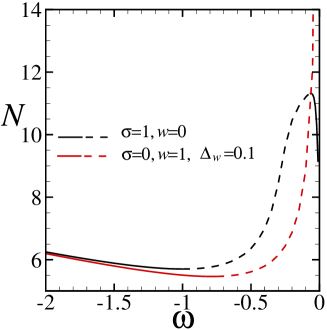
Figure 7: (Color online) The comparison of the numerically found dependence $N(\omega)$ in the linear lattice ($\sigma=0$), with the nonlinearity represented solely by the narrow nonlinear defect ($v=0,\Delta_{w}=0.1$)–red lines–with its counterpart in the usual defect-free DNLS lattice (black solid and dashed lines).

IV Localization-delocalization transition controlled by temporal modulations of the linear and nonlinear defect

IV.1 The variation of the linear defect

In this section, we consider effects of the hysteresis for the discrete solitons, induced by the adiabatic variation of the strength of the linear defect, $v(t)$, which eventually returns to the initial value, $v_{i}\equiv v(t=0)$, cf. Ref. BBK :

$$v(t)=v_{f}+(v_{i}-v_{f})|1-2t/t_{f}|.$$ (20)

Here $v_{f}\equiv v(t=t_{f}/2)$ corresponds to the turning point, $t=t_{f}/2$, while the return time is $t=t_{f}$. Note that the total norm remains a conserved quantity in the DNLS equation with the time-dependent strength of the local defect.

First, we consider the soliton for $v_{i}=0$, with the norm, $N_{s}$ (point A in Fig. 8), which precisely coincides with the minimum of the existence curve, but for $v=-1$ (point B). This means that, by taking $v_{i}=0$ and $v_{f}=-1$ in Eq. (20) at $t=t_{f}/2$, we may transfer the soliton from point A to B. As long as the soliton stays on the existence curve between these two points, it remains localized, featuring some changes of the profile, see details of dynamics in Fig. 9 (this is also valid for the dynamics between points A and C). However, if, in the framework of the same scenario, the amplitude of the defect falls below the critical value, $v_{f}<v_{\mathrm{cr}}$, which in the present case is $v_{\mathrm{cr}}=-1$, then the minimum of the existence curve turns out to be higher than the norm of the evolving mode, which is expected to trigger the delocalization.

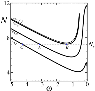
Figure 8: (Color online) The illustration of the transformation of the discrete soliton under the action of the adiabatic variation of the strength of the linear defect.

These assumptions were verified by means of the direct integration of Eq. (1) with the strength of the linear defect $v$ varying in time according to Eq. (20). The result is presented in Fig. 9, where the evolution of the density at the origin, $|u_{0,0}(t)|^{2}$, is shown for three values of the $v_{f}$, along with the corresponding initial and final profiles.

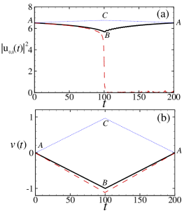
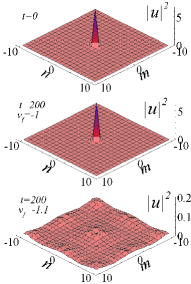
Figure 9: (Color online) (a) The evolution of the density at the origin, $|u_{0,0}(t)|^{2}$, corresponding to the time-modulation scenarios displayed in Fig. 8. The dark solid and blue dashed-dotted lines stand for the scenarios A-B-A (with $v_{f}=-1$) and A-C-A (with $v_{f}=1$), which are shown in panel (b) and in Fig. 8. The red dashed line corresponds to the case when the strength $v(t)$ temporarily falls to a value below the critical value, $v_{f}=-1.1<v_{\mathrm{cr}},$ which leads to the delocalization. In the right panels, initial (top) and final density profiles with $v_{f}=-1$ (middle) and $v_{f}=-1.1$ (bottom) are displayed.

IV.2 The variation of the nonlinear defect

Here we aim to consider effects produced by the adiabatic variation of the strength of the nonlinear defect, following the same scenario as in Eq. (20):

$$w(t)=w_{f}+(w_{i}-w_{f})|1-2t/t_{f}|,$$ (21)

with $w_{i}=w(t=0)$ and $w_{f}=w(t=t_{f}/2)$ corresponding to the initial strength and its value at the turning point, $t=t_{f}/2$, with the return to the initial value at $t=t_{f}$. As in the previous case, the norm of the solution remains conserved in the course of the evolution.

Again we start with the solution at $w_{i}=0$ (point A in Fig. 10) with the norm which coincides with the minimum of the existence curve for $w=-0.2$ (point B). This means that, by taking $w_{i}=0$ and $w_{f}=-0.2$ in Eq. (21) at time $t=t_{f}/2$, we will transfer the soliton from point A to point B, see Fig. 10. If the soliton stays on the existence curve between these two points, the solution always remains localized (see the dynamical picture in Fig. 11). However, if, for the same initial condition, the strength of the nonlinear defect is allowed to drop below the critical value, $w_{f}<w_{\mathrm{cr}}$, which in the present case is $w_{\mathrm{cr}}=-0.2$, then the minimum of the existence curve becomes higher than the norm of the solution, which again is expected to trigger the transition to the delocalization.

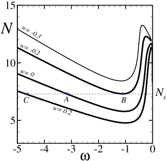
Figure 10: (Color online) The illustration of the soliton transformation under the action of the adiabatic variation of the strength of the nonlinear defect.

These assumption were verified through the direct integration of Eq. (1) with the strength of the nonlinear defect, $w$, varying in time according to Eq. (21). The results are presented in Fig. 11, where the evolution of the density at the origin, $|u_{0,0}(t)|^{2}$, is shown for three values of $w_{f}$.

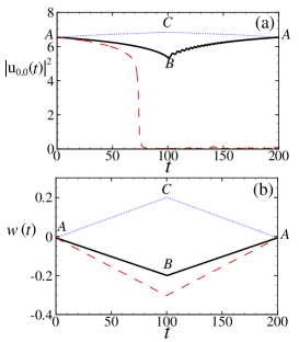
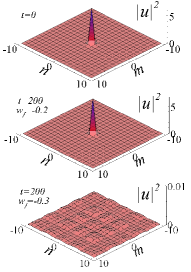
Figure 11: (Color online) The same as in Fig. 9, but for the temporal modulation of the nonlinear defect.

V Conclusion

In this work, we have considered the static and dynamical properties of 2D discrete solitons in the nonlinear lattice described by the DNLS (discrete nonlinear Schrödinger) equation, which includes the local linear or nonlinear defect. The solitons trapped around the defects were investigated using both the VA (variational approximation) and numerical methods, the VA showing good agreement with the numerical findings for sufficiently narrow solitons. Then, the analysis was extended to the model with the linear and nonlinear defects whose strength was subject to the slow variation in time. In the latter case, one of the possibilities is the controlled onset of the transition to delocalization.

The analysis reported in this work can be extended by considering combinations of linear and nonlinear defects, searching for symmetric, antisymmetric, and asymmetric modes trapped by symmetric pairs of defects, and analyzing other “management” schemes, with the defect strength subject to a time-periodic modulation.

Appendix A

Here we discuss some details on the continuation of solutions from the anti-continuum (AC) limit, which corresponds to the uncoupled lattice described by Eq. (1) and (5) with $J=0$ Panos . Looking for stationary modes in the form of Eq. (3), in the AC limit one obtains obvious exact solution for the one-site fundamental discrete soliton,

$$U_{m,n}=\left\{\begin{array}[]{ll}\pm\mathcal{A},&\mbox{if}\quad m=n=0;\\ 0,&\mbox{otherwise}.\end{array}\right.$$ (22)

where $\mathcal{A}\equiv\sqrt{-\left(\omega+v\right)/\left(\sigma+w\right)}$, see Ref. Alfimov and references therein. Then, by using the standard Newton-Raphson method, we gradually increase the coupling constant from $J=0$ to $J=1$, also increasing the width of the defect if needed [to proceed from the narrow defect (5) to the broader one (2)]. After that, by changing frequency $\omega$ of the solution, we obtain the dependence of norm $N$ on $\omega$, and also analyze the linear stability of the corresponding solutions, see the next Appendix.

Appendix B

To analyze the stability of solitons, we consider perturbed solutions,

$$u_{m,n}(t)=\left[U_{m,n}+a_{m,n}(t)\right]e^{-i\omega t},$$ (23)

Representing the small perturbations as $a_{m,n}(t)=\left(\alpha_{m,n}+i\beta_{m,n}\right)e^{\lambda t}$, substituting this into Eq. (1) and separating real and imaginary parts, we derive the following system,

$$\lambda\left(\begin{array}[]{l}\alpha\\ \beta\end{array}\right)=\left(\begin{array}[]{ll}0&L_{1}\\ -L_{3}&0\end{array}\right)\left(\begin{array}[]{l}\alpha\\ \beta\end{array}\right)$$ (24)

where $\lambda$ is the stability eigenvalue, and operators $L_{1}$ and $L_{3}$ are

$$L_{1} = \Delta_{2}+V_{m,n}-\omega+(\sigma+W_{m,n})\left(U_{m,n}\right)^{2},$$ (25)

$$L_{3} = \Delta_{2}+V_{m,n}-\omega+3(\sigma+W_{m,n})\left(U_{m,n}\right)^{2}.$$ (26)

Multiplying the first equation in system (24) by $-\lambda$ and than using the second equation, one arrives at the eigenvalue problem,

$$\Lambda\alpha=L_{1}L_{3}\alpha,$$ (27)

where $\Lambda=-\lambda^{2}$. The underlying stationary solution, $U_{m,n}$, is unstable if the spectrum of $\Lambda$ includes complex or negative real values.

References

- (1) F. Lederer, G. I. Stegeman, D. N. Christodoulides, G. Assanto, M. Segev, and Y. Silberberg, Phys. Rep. 463, 1 (2008).
- (2) A. Trombettoni and A. Smerzi, Phys. Rev. Lett. 86, 2353 (2001); F. Kh. Abdullaev, B. B. Baizakov, S. A. Darmanyan, V. V. Konotop, and M. Salerno, Phys. Rev. A 64 043606 (2001); E.G. Alfimov, P. G. Kevrekidis, V. V. Konotop, and M. Salerno, Phys. Rev. E 66, 046608 (2002).
- (3) O. Morsch and M. Oberthaler, Rev. Mod. Phys. 78, 179 (2006).
- (4) P. G. Kevrekidis, editor, The Discrete Nonlinear Schrödinger Equation: Mathematical Analysis, Numerical Computations, and Physical Perspectives (Springer: Berlin and Heidelberg, 2009).
- (5) T. Hattori, N. Tsurumachi, and H. Nakatsuka, J. Opt. Soc. Am. B 14, 348 (1997).
- (6) Y. Akahane, T. Asano, B. S. Song, and S. Noda, Nature 425, 944 (2003).
- (7) R. Colombelli, K. Srinivasan, M. Troccoli, O. Painter, C. F. Gmachl, D. M. Tennant, A. M. Sergent, D. L. Sivco, A. Y. Cho, and F. Capasso, Science 302, 1374 (2003).
- (8) H. Nakamura, Y. Sugimoto, K. Kanamoto, N. Ikeda, Y. Tanaka, Y. Nakamura, S. Ohkouchi, Y. Watanabe, K. Inoue, H. Ishikawa, and K. Asakawa,Opt. Exp. 12, 6606 (2004).
- (9) B. A. Malomed, Soliton Management in Periodic Systems (Springer: New York, 2006).
- (10) G. Kalosakas, K. Ø. Rasmussen, and A. R. Bishop, Phys. Rev. Lett. 89, 030402 (2002).
- (11) P. L. Christiansen, Yu. B. Gaididei, K. Ø. Rasmussen, V. K. Mezentsev, and J. Juul Rasmussen, Phys. Rev. B 54, 900 (1996).
- (12) M. I. Molina and Y. S. Kivshar, Phys. Rev. A 80, 063812 (2009).
- (13) M. I. Weinstein, Nonlinearity 12, 673 (1999); J.-K. Xue, A.-X. Zhang, and J. Liu, Phys. Rev. A 77, 013602 (2008).
- (14) C. Chong, R. Carretero-González, B. A. Malomed, and P. G. Kevrekidis, Physica D 238, 126 (2009).
- (15) Yu. V. Bludov, V. A. Brazhnyi, and V. V. Konotop, Phys. Rev. A 76, 023603 (2007).
- (16) Z. Chen, H. Martin, E. D. Eugenieva, J. Xu, and J. Yang, Opt. Exp. 13, 1816 (2005); D. N. Christodoulides and R. I. Joseph, Opt. Lett. 13, 794 (1988).
- (17) T. Mayteevarunyoo, B. A. Malomed, and M. Krairiksh, Phys. Rev. A 76, 053612 (2007).
- (18) G. Burlak and B. A. Malomed, Phys. Rev. 77, 053606 (2008).
- (19) G. L. Alfimov, V. A. Brazhnyi, and V. V. Konotop, Physica D 194, 127 (2004).