Image Separation using Wavelets and Shearlets

Abstract

In this paper, we present an image separation method for separating images into point- and curvelike parts by employing a combined dictionary consisting of wavelets and compactly supported shearlets utilizing the fact that they sparsely represent point and curvilinear singularities, respectively. Our methodology is based on the very recently introduced mathematical theory of geometric separation, which shows that highly precise separation of the morphologically distinct features of points and curves can be achieved by $\ell^{1}$ minimization. Finally, we present some experimental results showing the effectiveness of our algorithm, in particular, the ability to accurately separate points from curves even if the curvature is relatively large due to the excellent localization property of compactly supported shearlets.

1 Introduction

The task of separating an image into its morphologically different contents has recently drawn a lot of attention in the research community due to its significance for applications. In neurobiological imaging, it would, for instance, be desirable to separate ’spines’ (pointlike objects) from ’dendrites’ (curvelike objects) in order to analyze them independently aiming to detect characteristics of Alzheimer disease. Also, in astronomical imaging, astronomers would often like to separate stars from filaments for further analysis, hence again separating point- from curvelike structures. Successful methodologies for efficiently and accurately solving this task can in fact be applied to a much broader range of areas in science and technology including medical imaging, surveillance, and speech processing.

Although the problem of separating morphologically distinct features seems to be intractable – the problem is underdetermined, since there is only one known data (the image) and two or more unknowns – there has been extensive studies on this topic. The book by Meyer [18] initiated the area of image decomposition, in particular, the utilization of variational methods. Some years later, Starck, Elad, and Donoho suggested a different approach in [19] coined ‘Morphological Component Analysis’, which proclaims that such a separation task might be possible provided that we have prior information about the type of features to be extracted and provided that the morphological difference between those is strong enough. For the separation of point- and curvelike features, it was in fact recently even theoretically proven in [3] that $\ell_{1}$ minimization solves this task with arbitrarily high precision exploring a combined dictionary of wavelets and curvelets. Wavelets provide optimally sparse expansions for pointlike structures, and curvelets provide optimally sparse expansions for curvelike structures. Thus $\ell_{1}$ minimization applied to the expansion coefficients of the original image into this combined dictionary forces the pointlike structures into the wavelet part and the curvelike structures into the curvelet part, thereby automatically separating the image. An associated algorithmic approach using wavelets and curvelets has been implemented in MCALab.

Recently, a novel directional representation system – so-called shearlets – has emerged which provides a unified treatment of continuum models as well as digital models, allowing, for instance, a precise resolution of wavefront sets, optimally sparse representations of cartoon-like images, and associated fast decomposition algorithms; see the survey paper [11]. Shearlet systems are systems generated by one single generator with parabolic scaling, shearing, and translation operators applied to it, in the same way wavelet systems are dyadic scalings and translations of a single function, but including a directionality characteristic owing to the additional shearing operation (and the anisotropic scaling). The shearing operation in fact provides a more favorable treatment of directions, thereby ensuring a unified treatment of the continuum and digital realm as opposed to curvelets which are rotation-based in the continuum realm, see [1].

Thus, it is natural to ask whether also a combined dictionary of wavelets and shearlets might be utilizable for separating point- and curvelike features, the advantage presumably being a faster scheme, a more precise separation, and a direct applicability of theoretical results achieved for the continuum domain. And, in fact, the theoretical results from [3] based on a model situation were shown to also hold for a combined dictionary of wavelets and shearlets [2]. Moreover, numerical results give evidence to the superior behavior of shearlet-based decomposition algorithms when compared to curvelet-based algorithms; see [11] for a comparison of ShearLab with CurveLab.

In this paper, we will present a novel approach to the separation of point- and curvelike features exploiting a combined dictionary of wavelets and shearlets as well as utilizing block relaxation in a particular way. Numerical results give evidence that indeed the previously anticipated advantages hold true, i.e., that this approach is superior to separation algorithms using wavelets and curvelets such as MCALab in various ways, in particular, our algorithm is faster and provides a more precise separation, in particular, if the curvature of the curvilinear part is large. In the spirit of reproducible research [5], our algorithm is included in the freely available ShearLab toolbox.

This paper is organized as follows. In Section 2, we introduce the multiscale system of shearlets, and Section 3 reviews the mathematical theory of geometric separation of point- and curvelike features. Our novel algorithmic approach is presented in Section 4 with numerical results discussed in Section 5.

2 Shearlets

In most multivariate problems, important features of the considered data are concentrated on lower dimensional manifolds. For example, in image processing an edge is an 1D curve that follows a path of rapid change in image intensity. Recently, the novel directional representation system of shearlets [14, 8] has emerged to provide efficient tools for analyzing the intrinsic geometrical features of a signal using anisotropic and directional window functions. In this approach, directionality is achieved by applying integer powers of a shear matrix, and those operations preserve the structure of the integer lattice which is crucial for digital implementations. In fact, this key idea leads to a unified treatment of the continuum as well as digital realm, while still providing optimally sparse approximations of anisotropic features. As already mentioned before, shearlet systems are generated by parabolic scaling, shearing, and translation operators applied to one single generator. Let us now be more precise and formally introduce shearlet systems in 2D.

We first start with some definitions for later use. For $j\geq 0$ and $k\in\mathbb{Z}$, let

$$A_{2^{j}}=\begin{pmatrix}2^{j}&0\\ 0&2^{j/2}\end{pmatrix},\quad\tilde{A}_{2^{j}}=\begin{pmatrix}2^{j/2}&0\\ 0&2^{j}\end{pmatrix},\quad\text{and}\quad S_{k}=\begin{pmatrix}1&k\\ 0&1\end{pmatrix}.$$

We can now define so-called cone-adapted discrete shearlet systems, where the term ‘cone-adapted’ originates from the fact that these systems tile the frequency domain in a cone-like fashion. For this, let $c$ be a positive constant, which will later control the sampling density. For $\phi,\psi,\tilde{\psi}\in L^{2}({\mathbb{R}}^{2})$, the cone-adapted discrete shearlet system $SH(\phi,\psi,\tilde{\psi};c)$ is then defined by

$$SH(\phi,\psi,\tilde{\psi};c)=\Phi(\phi;c)\cup\Psi(\psi;c)\cup\tilde{\Psi}(\tilde{\psi};c),$$

where

$$\Phi(\phi;c) =\{\phi(\cdot-cm):m\in{\mathbb{Z}}^{2}\},$$

$$\Psi(\psi;c) =\{\psi_{j,k,m}=2^{\frac{3}{4}j}\psi(S_{k}A_{2^{j}}\,\cdot\,-cm):j\geq 0,|k|\leq\lceil 2^{{j/2}}\rceil,m\in{\mathbb{Z}}^{2}\},$$

$$\tilde{\Psi}(\tilde{\psi};c) =\{\tilde{\psi}_{j,k,m}=2^{\frac{3}{4}j}\tilde{\psi}(S^{T}_{k}\tilde{A}_{2^{j}}\,\cdot\,-cm):j\geq 0,|k|\leq\lceil 2^{{j/2}}\rceil,m\in{\mathbb{Z}}^{2}\}.$$

In [9], a comprehensive theory of compactly supported shearlet frames is provided, i.e., systems with excellent spatial localization. It should also be mentioned that in [12] a large class of compactly supported shearlet frames were shown to provide optimally sparse approximations of images governed by curvilinear structures, in particular, so-called cartoon-like images as defined in [1]. This fact will be explored in the sequel.

3 Mathematical Theory of Geometric Separation

In [19], a novel image separation method – Morphological Component Analysis (MCA) – based on sparse representations of images was introduced. In this approach, it is assumed that each image is the linear combination of several components that are morphologically distinct – for instance, points, curves, and textures. The success of this method relies on the assumption that each of the components is sparsely represented in a specific representation system. The key idea is then the following: Provided that such representation systems are identified, the usage of a pursuit algorithm searching for the sparsest representation of the image with respect to the dictionary combining all those specific representation systems will lead to the desired separation.

Various experimental results in [19] show the effectiveness of this method for image separation however without any accompanying mathematical justification. Recently, the first author of this paper and Donoho developed a mathematical framework in [3] within which the notion of successful separation can be made definitionally precise and can be mathematically proven in case of separating point- from curvelike features, which they coined Geometric Separation. One key ingredient of their analysis is the consideration of clustered sparsity properties measured by so-called cluster coherence. In this section, we briefly review this theoretical approach to the Geometric Separation Problem, which will serve as the foundation for our algorithm.

3.1 Model Situation

As a mathematical model for a composition of point- and curvelike structures, we consider the following two components: As a ‘point-like’ object, we consider the function ${\mathcal{P}}$ which is smooth except for point singularities and is defined by

$${\mathcal{P}}=\sum_{i=1}^{P}|x-x_{i}|^{-3/2}.$$

As a ‘curve-like’ object, we consider the distribution ${\mathcal{C}}$ with singularity along a closed curve $\tau:[0,1]\rightarrow\mathbb{R}^{2}$ defined by

$${\mathcal{C}}=\int\delta_{\tau(t)}dt.$$

Then our model situation is the sum of both, i.e.,

$$f={\mathcal{P}}+{\mathcal{C}}.$$ (1)

The Geometric Separation Problem now consists of recovering ${\mathcal{P}}$ and ${\mathcal{C}}$ from the observed signal $f$.

3.2 Chosen Dictionary

As we indicated before, it is now crucial to choose two representations systems each of which sparsely represents one of the morphologically different components in the Geometric Separation Problem. Our sparse approximation result, described in the previous section, suggests that curvilinear singularities can be sparsely represented by shearlets. On the other hand, it is well known that wavelets can provide optimally sparse approximations of functions which are smooth apart from point singularities. Hence, we choose the overcomplete system within which we will expand the signal $f$ as a composition of the following two systems:

• Orthonormal Separable Meyer Wavelets: Band-limited wavelets which form an orthonormal basis of isotropic generating elements.

• Bandlimited Shearlets: A directional and anisotropic tight frame generated by a band-limited shearlet generator $\psi$ defined in Section 2.

3.3 Subband Filtering

Since the scaling subbands of shearlets and wavelets are similar we can define a family of filters $(F_{j})_{j}$ which allows to decompose a function $f$ into pieces $f_{j}$ with different scales $j$ depending on those subbands. The piece $f_{j}$ associated to subband $j$ arises from filtering $f$ using $F_{j}$ by

$$f_{j}=F_{j}\ast f,$$

resulting in a function whose Fourier transform $\hat{f}_{j}$ is supported on the scaling subband of scale $j$ of the wavelet as well as the shearlet frame. The filters are defined in such way, that the original function can be reconstructed from the sequence $(f_{j})_{j}$ using

$$f=\sum_{j}F_{j}\ast f_{j},\quad f\in L^{2}(\mathbb{R}^{2}).$$

We can now exploit these tools to attack the Geometric Separation Problem scale-by-scale. For this, we filter the model problem (1) to derive the sequence of filtered images

$$f_{j}={\mathcal{P}}_{j}+{\mathcal{C}}_{j}\quad\text{for all scales}\,\,j.$$

3.4 $\ell_{1}$ Minimization Problem

Let now $\Phi_{1}$ and $\Phi_{2}$ be an orthonormal basis of band-limited wavelets and a tight frame of band-limited shearlets, respectively. Then, for each scale $j$, we consider the following optimization problem:

$$(\hat{W}_{j},\hat{S}_{j})=\text{argmin}_{W_{j},S_{j}}\|\Phi^{T}_{1}W_{j}\|_{1}+\|\Phi^{T}_{2}S_{j}\|_{1}\quad\text{subject to }\,\,f_{j}=W_{j}+S_{j}.$$ (2)

Notice that $\Phi^{T}_{1}W_{j}$ and $\Phi^{T}_{2}S_{j}$ are the wavelet and shearlet coefficients of the signals $W_{j}$ and $S_{j}$, respectively. Notice that our objective is not on searching for the sparsest expansion in a wavelet-shearlet dictionary, but on separation. Thus we can avoid an extensive, presumably numerically instable search by minimizing specific coefficients, namely the analysis in contrast to the synthesis coefficients, for each possible separation $f_{j}=W_{j}+S_{j}$.

We wish to further remark, that here the $\ell_{1}$ norm is placed on the analysis rather than the synthesis coefficients to avoid numerical instabilities due to the redundancy of the shearlet frame.

3.5 Theoretical Result

The theoretical result of the precision of separation of $f_{j}$ via (2) proved in [3] and [2] can now be stated in the following way:

Theorem 3.1 ([3] and [2])

Let $\hat{W}_{j}$ and $\hat{S}_{j}$ be solutions to the optimization problem (2) for each scale $j$. Then we have

$$\frac{\|{\mathcal{P}}_{j}-\hat{W}_{j}\|_{2}+\|{\mathcal{C}}_{j}-\hat{S}_{j}\|_{2}}{\|{\mathcal{P}}_{j}\|_{2}+\|{\mathcal{C}}_{j}\|_{2}}\rightarrow 0,\quad j\rightarrow\infty.$$

This result shows that the components ${\mathcal{P}}_{j}$ and ${\mathcal{C}}_{j}$ are recovered with asymptotically arbitrarily high precision at very fine scales. The energy in the pointlike component is completely captured by the wavelet coefficients, and the curvelike component is completely contained in the shearlet coefficients. Thus, the theory evidences that the Geometric Separation Problem can be satisfactorily solved by using a combined dictionary of wavelets and shearlets and an appropriate $\ell_{1}$ minimization problem.

3.6 Extensions

Our numerical scheme for image separation, which we will present in detail in the next section, will use a shift invariant wavelet tight frame and a compactly supported shearlet frame as opposed to orthonormal Meyer wavelets and band-limited shearlets required for Theorem 3.1. Hence this deserves some comments. Firstly, Theorem 3.1 is based on an abstract separation estimate which holds for any pair of frames, provided certain relative sparsity and cluster coherence conditions with respect to the components of the data to be separated are satisfied (cf. [3]). Secondly, using the recently introduced concept of sparsity equivalence (see [2, 10]), results requiring sparsity and coherence conditions can be transferred from one system (set of systems) to another by ‘merely’ considering particular decay conditions of the cross-Grammian matrix (matrices). We strongly believe that this framework allows a similar result as Theorem 3.1 for the pair of a shift invariant wavelet tight frame and a compactly supported shearlet frame. Since the focus of this paper is however on the introduction of the numerical scheme, such a highly technical, theoretical analysis is beyond the scope of this paper and will be treated in a subsequent work.

4 Our Algorithmic Approach to the Geometric Separation Problem

In this section, we present our algorithmic approach to the Geometric Separation Problem of separating point- from curvelike features by using a combined dictionary of wavelets and shearlets. The ingredients of the algorithm will be detailed below.

4.1 General Scheme

In practice, the observed signal $f$ is often contaminated by noise which requires an adaption of the optimization problem (2). As proposed in numerous publications, one typically considers a modified optimization problem – so-called Basis Pursuit Denoising (BPDN) – which can be obtained by relaxing the constraint in (2) in order to deal with noisy observed signals (see [6]). For each scale $j$, the optimization problem then takes the form:

$$(\hat{W}_{j},\hat{S}_{j})=\text{argmin}_{W_{j},S_{j}}\|\Phi^{T}_{1}W_{j}\|_{1}+\|\Phi^{T}_{2}S_{j}\|_{1}+\lambda\|f_{j}-W_{j}-S_{j}\|_{2}^{2}.$$ (3)

In this new form, the additional content in the image – the noise – characterized by the property that it can not be represented sparsely by either one of the two representation systems will be allocated to the residual $f_{j}-W_{j}-S_{j}$. Hence, performing this minimization, we not only separate point- and curvelike objects, which were modeled by ${\mathcal{P}}_{j}$ and ${\mathcal{C}}_{j}$ in Subsection 3.1, but also succeed in removing an additive noise component as a by-product. Of course, solving the optimization problem (3) for all relevant scales $j$ is computationally expensive.

4.2 Preprocessing

To avoid high complexity, we observe that the frequency distribution of point- and curvelike components is highly concentrated on high frequencies. Hence it would be essentially sufficient for achieving accurate separation to solve (3) for only sufficiently large scales $j$, as also evidenced by Theorem 3.1. This idea leads to a simplification of the problem (3) by modifying the observed signal $f$ as follows: We first consider bandpass filters $F_{0},\dots,F_{L}$, where $(F_{j})_{j=0,\dots,L}$ is the family of bandpass filters defined in Subsection 3.3 up to scale $L$, and $F_{0}$ is a lowpass filter. Thus the observed signal $f$ satisfies

$$f=\sum_{j=0}^{L}F_{j}\ast f_{j}\quad\text{with}\,\,f_{j}=F_{j}\ast f.$$

For each scale $j$, we now carefully choose a non-uniform weight $w_{j}>0$ satisfying, in particular, $w_{j}<w_{j^{\prime}}$, if $j<j^{\prime}$. These weights are then utilized for a weighted reconstruction of $f$ resulting in a newly constructed signal $\tilde{f}$ by computing

$$\tilde{f}=\sum_{j=0}^{L}w_{j}\cdot(F_{j}\ast f_{j}).$$ (4)

In this way, the two morphological components, namely points and curves, can be enhanced by suppressing the low frequencies.

While emphasizing that certainly other weights can be applied in our scheme, for the numerical tests presented in this paper we chose $L=3$, i.e., 4 subbands, and weights $w_{0}=0,w_{1}=0.1,w_{2}=0.7$, and $w_{3}=0.7$. This coincides with the intuition that a strong weight should be assigned to a band on which the power spectrum of the underlying morphological contents is highly concentrated. We do not claim that this is necessarily the optimal choice, and a comprehensive mathematical optimality analysis is beyond our reach at this moment. To our mind, the numerical results though justify this choice.

4.3 Solver for the $\ell_{1}$ Minimization Problem

Using the reweighted reconstruction of $f$ from (4) coined $\tilde{f}$, we now consider the following new minimization problem:

$$(\hat{W},\hat{S})=\text{argmin}_{W,S}\|\Phi^{T}_{1}W\|_{1}+\|\Phi^{T}_{2}S\|_{1}+\lambda\|\tilde{f}-W-S\|_{2}^{2}.$$ (5)

Note that the frequency distribution of $\tilde{f}$ is highly concentrated on the high frequencies – in other words, scaling subbands of large scales $j$ –, and Theorem 3.1 justifies our expectation of a very precise separation using $\tilde{f}$ instead of $f$. Even more advantageous, the reduced problem (5) no longer involves different scales $j$, and hence can be efficiently solved by various fast numerical schemes. In our separation scheme, we use the same optimization method as the one used in MCALab to solve (5) now applied to a combined wavelet-shearlet dictionary. We refer to [7] for a detailed description of an algorithmic approach to solve (5); see also [6]. In the following subsections, we discuss the particular form of the matrices $\Phi^{T}_{1}$ and $\Phi^{T}_{2}$ which encode the wavelet and shearlet transform in the minimization problem (5) we aim to solve.

4.4 Wavelet Transform

Let us start with the wavelet transform. The undecimated digital wavelet transform is certainly the most fitting version of the wavelet transform for the filtering of data, and hence this is what we utilize also here. This transform is obtained by skipping the subsampling, thereby yielding an overcomplete transform, which in addition is shift-invariant. The redundancy factor of this transform is $3J+1$, where $J$ is the number of decomposition levels. We refrain from further details and merely refer the reader to [17].

4.5 Shearlet Transform

For the shearlet transform, we employ the digital shearlet transform implemented by 2D convolution with discretized compactly supported shearlets, which was introduced in [16], see also [13]. In the earlier work [15], an faithful digitalization of the continuum domain shearlet transform using compactly supported shearlets generated by separable functions has been developed. However, firstly, this algorithmic realization allows only a limited directional selectivity due to separability and, secondly, compactly supported shearlets generated by separable functions do not form a tight frame which causes an additional computational effort to approximate the inverse of the shearlet transform by iterative methods. These problems have been resolved in [16, 13] by using non-separable compactly supported generators, and we now summarize this procedure.

In the sequel, we will discuss the implementation strategy for computing the shearlet coefficients $\langle f,\psi_{j,k,m}\rangle$ only for $\psi_{j,k,m}\in\Psi(\psi,1)$. The same procedure can be applied to shearlets in $\tilde{\Psi}(\tilde{\psi},1)$ except for switching the role of variables. Without loss of generality, let $j/2$ be an integer. For $J>0$ fixed, assume that $f(x)=\sum_{n\in\mathbb{Z}^{2}}f_{J}(n)2^{L}\phi(2^{L}x-n),$ where $\phi$ is a 2D separable scaling function of the form $\phi_{1}(x_{1})\phi_{1}(x_{2})$ satisfying

$$\phi(x)=\sum_{n\in\mathbb{Z}^{2}}h(n)2\phi(2x-n).$$ (6)

Let $\psi$ be a 2D separable wavelet defined by $\psi(x_{1},x_{2})=\psi_{1}(x_{1})\phi_{1}(x_{2})$, where $\psi_{1}$ is a 1D wavelet. Further, assume that $\psi$ can be written as

$$\psi(x)=\sum_{n\in\mathbb{Z}^{2}}w(n)2\phi(2x-n),$$ (7)

where $w(n)$ are 2D separable wavelet filter coefficients associated with scaling filter coefficients $h(n)$. For each $j\geq 0$, define the (non-separable) shearlet generator $\psi^{\text{non}}_{j}$ by

$$\hat{\psi}^{\text{non}}_{j}(\xi)=P_{J-j/2}(\xi)\hat{\psi}(\xi),$$ (8)

where $P_{\ell}(\xi)=P(2^{\ell+1}\xi_{1},\xi_{2})$ for $\ell\geq 0$ and the trigonometric polynomial $P$ is a 2D fan filter (c.f. [4]). To implement $\langle f(\cdot),\psi^{\text{non}}_{j,k,m}(\cdot)\rangle=\langle f(\cdot),\psi^{\text{non}}_{j,0,m}(S_{2^{-j/2}k}\cdot)\rangle,$ we make two observations: Firstly, the functions $\psi^{\text{non}}_{j,0,m}$ are wavelets generated by refinement equations (6), (7) and (8). Thus, for each $j$, there exists an associated 2D wavelet filter $w_{j}$. Secondly, the shear operator $S_{2^{-j/2}k}$ can be faithfully discretized by the digital shear operator $S^{d}_{2^{-j/2}k}$ (see [15, 16], also [13]). The digital (non-separable) shearlet transform is then, using the shearlet filters $\psi^{d}_{j,k}=S^{d}_{2^{-j/2}k}(w_{j})$, defined by

$$SH(f_{J})(m_{1},m_{2})=(f_{J}*\psi^{d}_{j,k})(2^{J-j}m_{1},2^{J-j/2}m_{2})\quad\text{for}\,\,f_{J}\in\ell^{2}(\mathbb{Z}^{2}).$$

If downsampling by $A_{2^{j}}$ is omitted, a shift invariant shearlet transform $(f_{J}*\psi^{d}_{j,k})(m_{1},m_{2})$ is obtained, in which case dual shearlet filters $\tilde{\psi}^{\text{d}}_{j,k}$ can be easily computed by deconvolution. We then obtain the reconstruction formula

$$f_{J}=\sum_{j,k}(f_{J}*\psi^{\text{d}}_{j,k}(-\,\cdot))*\tilde{\psi}^{\text{d}}_{j,k}.$$

5 Numerical Results

In this section, we present and discuss some numerical results of our proposed scheme for separating point- and curvelike features. In each experiment we compare our scheme, which is freely available in the ShearLab toolbox, with the separation algorithm MCALab. In contrast to our algorithm, MCALab uses wavelets and curvelets to separate point- and curvelike components, and we refer to [7] for more details on the algorithm.

5.1 Comparison by Visual Perception

Aiming first at comparison by visual perception, we choose an artificial image $I$ composed of two subimages $P$ and $C$, where $P$ solely contains pointlike structures and $C$ different curvelike structures (see Figures 1(a) and (b)). We further add white Gaussian noise to $I=P+C$, shown in Figure 1(c).

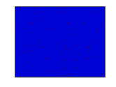
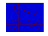
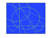
Figure 1: (a) P: Image of points. (b) C: Image of curves. (c) Noisy image (512 $\times$ 512).

Our scheme consists of two parts: Preprocessing of the image as described in Subsection 4.2, followed by separation using a combined wavelet-shearlet dictionary as described in Subsections 4.3-4.5. First, we will focus on the preprocessing step, and apply MCALab with and without our preprocessing step – due to limited space we just mention that our scheme is similarly positively affected by preprocessing. Figures 2(a) and (b) then visually indicate that preprocessing indeed significantly improves the accuracy of separation.

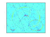
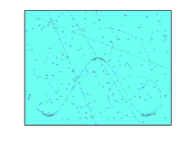
Figure 2: (a) Pointlike image component extracted by MCALab without preprocessing. (b) Pointlike image component extracted by MCALab with preprocessing.

To achieve a fair comparison, we now apply both schemes to the same preprocessed image as defined in (4). Figures 3 (a)-(d) and Figures 4(a)-(b) show the comparison results. In Figure 3(c), it can be observed that the curvelet transform performs well for extracting lines due to excellent directional selectivity. However, some part of the curve is missed and appears in the pointlike part, see also Figure 4(a). This error becomes worse with growing curvature. In contrast to this, compactly supported shearlets provide much better spatial localization than (band-limited) curvelets, which positively affects the capturing of localized features of the curve as illustrated in Figure 3(d) and Figure 4(b). Hence, with respect to this visual comparison, our scheme outperforms MCALab, in particular, when curves with large curvature are present.

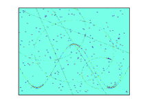
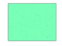
Figure 3: (a) MCALab: Pointlike component. (b) Our scheme: Pointlike component. (c) MCALab: Curvelike component. (d) Our scheme: Curvelike component.

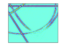
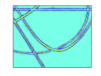
Figure 4: Zoomed images: (a) MCALab. (b) Our scheme.

5.2 Comparison by Quantitative Measures

We now put the comparison on more solid ground by introducing two quantitative measures for analyzing how accurate our scheme as compared to MCALab extracts points and curves.

To define our first quantitative measure, let $P$ and $C$ be (binary) images containing points and curves, respectively, with image domain $\Omega\subset\mathbb{Z}^{2}$, and let $\hat{P}$ and $\hat{C}$ be the separated images from $I=P+C+\text{noise}$ by the separation scheme to be analyzed. Letting $T\geq 0$, $\text{B}_{T}$ be defined by

$$\text{B}_{T}(I)=\chi_{\{n\in\Omega:I(n)\geq T\}},\quad\text{for a 2D image}\,\,I,$$

and $g$ be a 2D discrete Gaussian filter, we introduce the test measures

$$M_{p}(\hat{P})(T)=\frac{\|g*P-g*(\text{B}_{T\cdot\max(\hat{P})}(\hat{P}))\|_{2}}{\|g*P\|_{2}}$$

and

$$M_{c}(\hat{C})(T)=\frac{\|g*C-g*(\text{B}_{T\cdot\max(\hat{C})}(\hat{C}))\|_{2}}{\|g*C\|_{2}}.$$

Using $P$ and $C$ as given by Figure 1, the graphs of the error functions $M_{p}(\hat{P})$ and $M_{c}(\hat{C})$ for our scheme and MCALab are plotted in Figure 5 depending on the threshold parameter $0<T<1$.

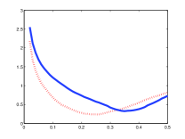
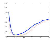
Figure 5: (a) Graph of quantitative measure $T\mapsto M_{p}(\hat{P})(T)$: Our scheme (dashed curve) and MCALab (solid curve). (b) Graph of quantitative measure $T\mapsto M_{p}(\hat{C})(T)$: Our scheme (dashed curve) and MCALab (solid curve).

These figures imply that our scheme outperforms MCALab with respect to this quantitative measure.

As our second quantitative measure, we will use the running time of each scheme. With respect to this comparison measure, MCALab runs 182.19 sec (30 iterations) to produce the test results while our scheme takes 135.37 sec (15 iterations). The running time was computed by taking the average over 10 runs. Again, with respect to this measure our scheme performs superior.

6 Application in Neurobiology

To test the performance of our scheme on real-world images, we apply it to an image of a neuron generated by fluorescence microscopy (Figure 6(a)), which is composed of ‘spines’ (pointlike features) and ‘dendrites’ (curvelike features). Figures 6(b) and (c) show the extracted images containing spines and dendrites, respectively.

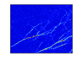
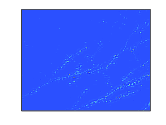
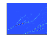
Figure 6: (a) Image of neuron. (b) Extracted spines. (c) Extracted dendrites.

7 Conclusion

In this paper, we introduced a novel methodology for separating images into point- and curvelike features based on the new paradigm of sparse approximation and using $\ell_{1}$ minimization. In contrast to other approaches, our algorithm utilizes a combined dictionary consisting of wavelets and shearlets, implemented as shift-invariant transforms, and is based on a mathematical theory. The excellent localization property of compactly supported shearlets allows shearlets to capture the curvelinear part very accurately and efficiently, even if the curvature is relatively large. Numerical results show that our scheme extracts point- and curvelike features more precise and uses less computing time than the state-of-the-art algorithm MCALab, which is based on wavelets and curvelets.

References

- [1] E. J. Candés and D. L. Donoho, New tight frames of curvelets and optimal representations of objects with piecewise singularities, Comm. Pure and Appl. Math. 56 (2004), 216–266.
- [2] D. L. Donoho and G. Kutyniok, Geometric Separation using a Wavelet-Shearlet Dictionary, SampTA’09 (Marseille, France, 2009), Proc., 2009.
- [3] D. L. Donoho and G. Kutyniok, Microlocal analysis of the geometric separation problem, preprint.
- [4] M. N. Do and M. Vetterli, The contourlet transform: An efficient directional multiresolution image representation, IEEE Trans. Image Process. 14 (2005), 2091–2106.
- [5] D. L. Donoho, A. Maleki, M. Shahram, V. Stodden, and I. Ur-Rahman, Fifteen years of reproducible research in computational harmonic analysis, Comput. Sci. Engrg. 11 (2009), 8–18.
- [6] M. Elad, Sparse and redundant representations, Springer, New York, 2010.
- [7] M.J. Fadilli, J.-L Starck, M. Elad, and D. L. Donoho, MCALab: Reproducible research in signal and image decomposition and inpainting, IEEE Comput. Sci. Eng. Mag. 12 (2010), 44–63.
- [8] K. Guo, G. Kutyniok, and D. Labate, Sparse multidimensional representations using anisotropic dilation and shear operators, Wavelets and Splines (Athens, GA, 2005), Nashboro Press, Nashville, TN, 2006, 189–201.
- [9] P. Kittipoom, G. Kutyniok, and W.-Q Lim, Construction of compactly supported shearlet frames, preprint.
- [10] G. Kutyniok, Sparsity equivalence of anisotropic decompositions, preprint.
- [11] G. Kutyniok, J. Lemvig, and W.-Q Lim, Compactly Supported Shearlets, Approximation Theory XIII (San Antonio, TX, 2010), Springer, to appear.
- [12] G. Kutyniok and W.-Q Lim, Compactly supported shearlets are optimally sparse, J. Approx. Theory, to appear.
- [13] G. Kutyniok, W.-Q Lim, and X. Zhuang, Digital Shearlet Transforms, in: Shearlets: Multiscale Analysis for Multivariate Data, Springer, New York, to appear.
- [14] D. Labate, W.-Q Lim, G. Kutyniok, and G. Weiss. Sparse multidimensional representation using shearlets, in Wavelets XI, edited by M. Papadakis, A. F. Laine, and M. A. Unser, SPIE Proc., 5914, SPIE, Bellingham, WA, 2005, 254–262,
- [15] W.-Q Lim, The discrete shearlet transform: A new directional transform and compactly supported shearlet frames, IEEE Trans. Image Proc. 19 (2010), 1166–1180.
- [16] W.-Q Lim, Shift Invariant Shearlet Transform, preprint.
- [17] S. Mallat, A wavelet tour of signal processing, Academic Press, Inc., San Diego, CA, 1998.
- [18] Y. Meyer, Oscillating Patterns in Image processing and nonlinear evolution equations, University Lecture Sereis, Amer. Math. Soc. 22 (2002).
- [19] J.-L Starck, M. Elad, and D. Donoho, Image decomposition via the combination of sparse representation and a variational approach, IEEE Trans. Image Proc. 14 (2005), 1570–1582.