Composite gravitational-wave detection of compact binary coalescence

Abstract

The detection of gravitational waves from compact binaries relies on a computationally burdensome processing of gravitational-wave detector data. The parameter space of compact-binary-coalescence gravitational waves is large and optimal detection strategies often require nearly redundant calculations. Previously, it has been shown that singular value decomposition of search filters removes redundancy. Here we will demonstrate the use of singular value decomposition for a composite detection statistic. This can greatly improve the prospects for a computationally feasible rapid detection scheme across a large compact binary parameter space.

I Introduction

Ground-based laser-interferometric gravitational-wave detectors have demonstrated sensitivity to gravitational-wave strain at the level of $10^{-22}$ or better over a band from $80-1000$ Hz The LIGO Scientific Collaboration (2009a); Acernese and et al (2008); Grote and the LIGO Scientific Collaboration (2010). Later this decade advanced detectors will surpass the present sensitivity by a factor of $\sim 10$ The LIGO Scientific Collaboration (2009b); The Virgo Scientific Collaboration (2005). One of the most promising sources of gravitational waves is the merger of two compact objects Cutler et al. (1993). Advanced detectors are expected to detect on the order of 40 neutron star - neutron star merger events per year Kopparapu et al. (2008); The LIGO Scientific Collaboration (2010) and a similar number of mergers involving black holes. The exact parameters of the signals, such as mass and spin of the component objects, will not be known ahead of time. Therefore, the optimal detection strategy must include the possibility of detecting signals with unknown parameters. Matched filtering has been employed to search this parameter space Finn and Chernoff (1993); Allen et al. (2005). The parameter space is explored by choosing a discrete set of filters that guarantees that all signals within the parameter space are found with a signal-to-noise ratio (SNR) greater than $\sim 97\%$ Owen (1996) of the maximum possible. Recently it has been shown that the use of singular value decomposition can reduce the number of filters necessary to search the parameter space Cannon et al. (2010). This paper extends that work to explore use of the singular value decomposition (SVD) filter outputs for detection without reconstructing the physical template waveforms.

If one is interested only in knowing whether any of the signals are present, and not which one is present, then the problem of detection decouples from that of parameter estimation. Wainstein and Zubakov (1962) Wainstein and Zubakov (1962) describe the problem of detecting any of several signals without concern for parameter estimation as composite detection. This paper will explore the composite detection of compact binary signals using the techniques proposed in Cannon et al. (2010). We find that the composite detection statistics explored produce a lower detection efficiency at a fixed false alarm rate than traditional approaches. However when combined hierarchically with traditional approaches, the combined approach can perform as well at low false alarm rate, but with reduced computational cost.

II Composite detection of compact binary signals

We will consider an unknown gravitational wave signal arising from a compact binary coalescence in the digitized gravitational-wave detector output as a vector of data points parameterized by an unknown amplitude $A$ and a collection of unknown parameters $\bar{\theta}$ (e.g., the masses of the component bodies) that determine the shape of the signal. We will denote this signal as $A{\bf s}(\bar{\theta})$. Both the amplitude and shape parameters are not known a priori. The relative frequency of parameters in the population is described by the probability density function $p(A,\bar{\theta})$. We will assume the joint distribution $p(A,\bar{\theta})$ is separable, that is $p(A,\bar{\theta})=p(A)p(\bar{\theta})$. This is not generally true globally across the parameter space, but should be roughly true locally. We will denote the vector of discretely time-sampled strain data as ${\bf h}$. In addition to containing normally distributed noise, ${\bf n}$, ${\bf h}$ will possibly contain the gravitational-wave signal,

$${\bf h}={\bf n}+A{\bf s}(\bar{\theta}).$$ (1)

Assuming the noise has unit variance and ${\bf s}(\bar{\theta})$ is normalized such that the inner-product of it with itself is unity, $A$ is the expected value for the SNR of a signal after optimally filtering.

The optimal detection statistic is the marginalized likelihood

$$\Lambda=\frac{p({\bf h}|{\bf s})}{p({\bf h}|{\bf 0})},$$ (2)

where $p({\bf h}|{\bf s})$ is the probability of obtaining ${\bf h}$ given the presence of any signal, with the signal parameters $A,\bar{\theta}$ integrated out

$$p({\bf h}|{\bf s}) = \int_{V}\int_{-\infty}^{+\infty}p({\bf h}|A,\bar{\theta})p(\bar{\theta})p(A)\,\mathrm{d}A\,\mathrm{d}\bar{\theta},$$ (3)

and $p({\bf h}|0)$ is the probability of obtaining ${\bf h}$ in the absence of any signal. The marginalized likelihood increases as the probability of the data containing a signal increases. For white noise,

$$p({\bf h}|0)\propto\exp\left(-\frac{1}{2}{\bf h}^{\mathrm{T}}{\bf h}\right).$$ (4)

This white noise form is also valid for colored noise cases if one applies the linear whitening transformation to the data ${\bf h}$. In the frequency domain, this transformation divides the data by the amplitude spectral density of the noise. Our goal is to find a computationally inexpensive approximation to this optimal detection statistic using the SVD-reduced filter set described in Cannon et al. (2010).

II.1 Expansion of the marginalized likelihood

In this section we will consider an expansion of the marginalized likelihood and show that it gives rise to a detection statistic that exploits the SVD filter basis.

For simplicity we will assume that the signal parameters $\bar{\theta}$ take on discrete values  so that we may index different signals as $\bf{s}_{i}$. We will also assume that the amplitude, $A$, does not depend on the signal index $i$. The detector output now has the form

$${\bf h}={\bf n}+A{\bf s_{i}}.$$ (5)

We don’t know a priori which signal ${\bf s_{i}}$ is present in the data. The marginalized likelihood Finn and Chernoff (1993) is

$$\Lambda\propto\sum_{j}\exp[A{\bf h}\cdot{\bf s_{j}}],$$ (6)

where the integral in (3) is replaced by a sum over all possible templates ${\bf s_{j}}$. Expanding the exponential to second order yields

$$\Lambda\stackrel{{\scriptstyle\sim}}{{\propto}}\sum_{j}\left[1+A{\bf h}\cdot{\bf s_{j}}+\frac{1}{2}A^{2}({\bf h}\cdot{\bf s_{j}})^{2}\right].$$ (7)

The first order term is oscillatory and contributes little to the sum. We thus ignore it and define the approximate likelihood as $\Lambda^{\prime}$

$$\Lambda^{\prime}:=\sum_{j}({\bf h}\cdot{\bf s_{j}})^{2}.$$ (8)

Using the change of basis described in Cannon et al. (2010), where

$${\bf s_{j}} = \sum_{k}v_{jk}\sigma_{k}{\bf u_{k}},$$ (9)

the approximate likelihood expression (8) simplifies to

$$\Lambda^{\prime} = \sum_{k}(\sigma_{k}{\bf h}\cdot{\bf u_{k}})^{2},$$ (10)

due to the properties of the orthonormal matrix $v_{jk}$. (10) has no dependence on the original parameter index $j$. As was shown in Cannon et al. (2010), fewer filters are required using the ${\bf u_{k}}$ basis, therefore the sum over $k$ has fewer terms than the original sum over $j$. Unfortunately higher order terms in the expansion of (7) do not simplify as well. It is possible to derive detection statistics that perform better than (10) while still exploiting the reduced filter set; one such example is shown in the next section.

II.2 Assuming the signal probability distribution is a multi-variate normal distribution

In this section we explore approximating the signal probability $p({\bf h}|{\bf s})$ in (3) as a multivariate normal distribution. This will result in a different detection statistic that still exploits the SVD filter basis.

We begin by assuming the signal probability (3) has the form

$$p({\bf h}|{\bf s})\propto\exp\left(-\frac{1}{2}{\bf h}^{\mathrm{T}}{\bf C}^{-1}{\bf h}\right),$$ (11)

whose covariance matrix ${\bf C}$ of second-order moments completely defines it. The covariance matrix is

$$C_{ij} = \mathrm{cov}(h_{i},h_{j})$$ (12)

$$= \left\langle(n_{i}+As_{i}(\bar{\theta})+)(n_{j}+As_{j}(\bar{\theta}))\right\rangle$$

$$= \left\langle n_{i}n_{j}\right\rangle+\left\langle A^{2}\right\rangle\left\langle s_{i}(\bar{\theta})s_{j}(\bar{\theta})\right\rangle$$

$$= \delta_{ij}+\left\langle A^{2}\right\rangle\int_{V}s_{i}(\bar{\theta})s_{j}(\theta)p(\bar{\theta})\,\mathrm{d}\bar{\theta},$$

where $\left\langle A^{2}\right\rangle=\int_{-\infty}^{+\infty}A^{2}p(A)\,\,\mathrm{d}A$ and we have assumed the independence of the variables $A$, $\bar{\theta}$ and $n_{i}$.

Using (4) and (11), we compute the logarithm of the marginalized likelihood, $\Lambda$. This is monotonic in $\Lambda$ and therefore is sufficient to use as a ranking statistic

$$\ln\Lambda\propto\Gamma:={\bf h}^{\mathrm{T}}\left({\bf I}-{\bf C}^{-1}\right){\bf h}.$$ (13)

The performance of (13) depends on the waveform population; we will assess it for simple but realistic cases in Sec. III.

We compute ${\bf C}$ by drawing $N$ samples of $\bar{\theta}$ distributed according to $p(\bar{\theta})$. We assume a signal population that is distributed according to our ability to distinguish signals, which is approximated by the filter banks described in Owen (1996). This definition of the signal population is approximately uniform in the $\bar{\theta}$ distribution for sufficiently small regions of parameter space. The integral in (12) is then approximated by a summation over these samples,

$$C_{ij}=\delta_{ij}+\frac{\left\langle A^{2}\right\rangle}{N}\sum^{N}_{k=1}s_{i}(\theta_{k})s_{j}(\theta_{k})$$

$${\bf C}={\bf I}+\frac{\left\langle A^{2}\right\rangle}{N}\sum_{k=1}^{N}{\bf s}^{\mathrm{T}}(\theta_{k}){\bf s}(\theta_{k}),$$ (14)

where $\theta_{k}$ are discrete values of $\bar{\theta}$ and ${\bf s}(\theta_{k})$ is a row vector of the time samples $s_{i}(\theta_{k})$. By defining the matrix $S_{ik}=s_{i}(\theta_{k})$ we can simplify the notation to

$${\bf C}={\bf I}+\frac{\left\langle A^{2}\right\rangle}{N}{\bf S}^{\mathrm{T}}{\bf S}.$$ (15)

This is precisely the arrangement of the signal matrix proposed in Cannon et al. (2010). As in (9), we use the SVD to decompose the signal matrix ${\bf S}$ (here written in matrix notation but equivalent to (9)),

$${\bf S}={\bf V}{\bf\Sigma}{\bf U}^{\mathrm{T}},$$ (16)

where ${\bf V}$ and ${\bf U}$ are unitary matrices and ${\bf\Sigma}$ is a diagonal matrix of the singular values of ${\bf S}$, referred to by components ${\sigma_{k}}$ in the Sec. II.1. ${\bf U}$ is the matrix of the orthonormal basis vectors ${\bf u_{k}}$ described in the previous section. Then we note that

$${\bf I}-{\bf C}^{-1} ={\bf I}-\left({\bf I}+\frac{\left\langle A^{2}\right\rangle}{N}{\bf S}^{\mathrm{T}}{\bf S}\right)^{-1}$$

$$={\bf I}-\left({\bf I}+\frac{\left\langle A^{2}\right\rangle}{N}{\bf U}{\bf\Sigma}^{2}{\bf U}^{\mathrm{T}}\right)^{-1}$$

$$={\bf U}\left({\bf I}-\left({\bf I}+\frac{\left\langle A^{2}\right\rangle}{N}{\bf\Sigma}^{2}\right)^{-1}\right){\bf U}^{\mathrm{T}},$$ (17)

where we have used ${\bf U}{\bf U}^{\mathrm{T}}={\bf U}^{\mathrm{T}}{\bf U}={\bf I}$. Let us define a diagonal matrix ${\bf J}$

$$J_{kk} :=1-\left(1+\frac{\left\langle A^{2}\right\rangle}{N}\sigma_{k}^{2}\right)^{-1}$$

$$=\frac{\sigma_{k}^{2}}{\sigma_{k}^{2}+\frac{N}{\left\langle A^{2}\right\rangle}.}$$ (18)

With this definition the approximate detection statistic (13) can be written as

$$\Gamma = {\bf h}^{\mathrm{T}}{\bf U}{\bf J}{\bf U}^{\mathrm{T}}{\bf h},$$ (19)

which, in the notation of the previous section, is

$$\Gamma = \sum_{k}\frac{\sigma_{k}^{2}}{\sigma_{k}^{2}+N/{\langle A^{2}\rangle}}({\bf h}\cdot{\bf u_{k}})^{2}.$$ (20)

It is worth noting the limits of this expression for low and high amplitude signals (small and large values of $A$),

$$\lim_{A\to 0}\Gamma=\sum_{k}\sigma_{k}^{2}({\bf h}\cdot{\bf u_{k}})^{2},$$ (21a)

$$\lim_{A\to\infty}\Gamma=\sum_{k}({\bf h}\cdot{\bf u_{k}})^{2}.$$ (21b)

The $A\to 0$ limit is exactly the same result as the second order approximation derived in the previous section. In this limit the most important filters (i.e., those with larger singular values) contribute more to the composite detection statistic. The $A\to\infty$ limit in (21b) reduces the composite detection statistic to the sum of squares of the orthogonal filter outputs, $({\bf h}\cdot{\bf u_{j}})$. This detection statistic is equivalent to the excess power statistic obtained in Anderson et. al for the detection of waveforms of known bandwidth and duration (Anderson et al., 2001, equation (2.10)). Here, instead of projecting the data onto a basis that spans a time-frequency tile, we project the data onto a basis that span the space of CBC waveforms. The essential difference between (20) and the excess power statistic of Anderson et. al is that (20) folds in knowledge of the relative probability that the waveforms we seek match any of the basis vectors individually, whereas the target waveforms in Anderson et al. (2001) are assumed to match the basis vectors of the time-frequency tile with equal probability.

Fig. 1 presents an example of the components of (II.2) for the small and large amplitude limits, and for an amplitude of 20. These were produced using the signal matrix described in Sec. III.1.

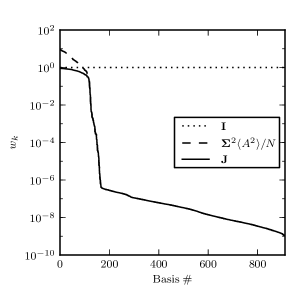
Figure 1: The coefficients $w_{k}$ used to construct the composite detection statistic as a function of basis vector number, ordered by their singular value. The solid trace shows the coefficients we obtain from (II.2) assuming a signal amplitude $A=20$. The dashed trace shows the singular values squared, the choice of coefficients given in (10). The dotted trace shows “the excess power” choice of coefficients, which are unity for all basis vectors.

III Operating characteristics of the proposed composite detection statistics

In this section we explore the performance of the proposed detection statistic (20). We begin by establishing the framework with which we conduct simulations to produce Receiver Operator Characteristic (ROC) curves. These indicate the probability of detection versus the probability of false alarm. We then present some practical scenarios in which to understand these results.

We begin by assuming the detector data ${\bf h}$ has the form of (5) modified to allow an ambiguous phase

$${\bf h}={\bf n}+A{\bf s_{i(0)}}+B{\bf s_{i(\pi/2)}}.$$ (22)

Under ideal situations the signal ${\bf s_{i}}$ could be recovered by a matched filter with an SNR of $\sqrt{A^{2}+B^{2}}$. According to Cannon et al. (2010) the signal ${\bf s_{i}}$ can be decomposed into orthogonal basis functions using the singular value decomposition such that

$${\bf s_{i(0)}} = \sum_{j}v^{ij}_{(0)}\sigma_{j}{\bf u_{j}},$$ (23)

$${\bf s_{i(\pi/2)}} = \sum_{j}v^{ij}_{(\pi/2)}\sigma_{j}{\bf u_{j}}.$$ (24)

This leads to the following expression of the composite detection statistic for (22)

$$\Gamma^{2}_{i} = \sum_{k}w_{k}({\bf h}\cdot{\bf u_{k}})^{2}$$

$$= \sum_{k}w_{k}\left[Av^{ik}_{(0)}\sigma_{k}+Bv^{ik}_{(\pi/2)}\sigma_{k}+n_{k})\right]^{2},$$

$$w_{k} = \frac{\sigma_{k}^{2}}{\sigma_{k}^{2}+N/A^{2}},$$ (25)

where $n_{k}$ is a random number drawn from a unit variance Gaussian distribution. We have made use of the fact that $({\bf u_{i}}\cdot{\bf u}_{j})=\delta_{ij}$.

In order to assess the operating characteristics of (20) we simulate several instances of signals and several instances of noise. We then compare the number of noise trials that produce a value of (20) greater than some threshold $\Gamma^{*}$ with the number of signal, plus noise, trials that produce values above the same threshold. This allows us to parameterize the detection probability versus false alarm probability using the value of $\Gamma^{*}$.

III.1 Simulations

In this section we simulate the procedure described above. Our goals are the following. First we explore how the detection probability of (20) varies of as a function of $A$ at a fixed false alarm probability. We verify that it peaks when the simulated signal amplitude is equal to $A$. We then compare the performance of (20) with standard matched filtering results. We find, to no surprise that (20) alone performs worse. However, we also find that by using (20) to hierarchically reconstruct the physical template SNR the same detection probability can be reached for sufficiently low false alarm probability.

In order to conduct these tests, we apply the singular value decomposition to binary neutron star (BNS) waveforms with chirp masses $1.125M_{\odot}\leq M_{c}<1.240M_{\odot}$ and component masses $1M_{\odot}\leq m_{1},m_{2}<3M_{\odot}$ Cannon et al. (2010). The number of templates required to hexagonally cover this range in parameters using a minimal match of $96.8\%$ is $M=456$, which implies a total number of single-phase filters $N=912$. These non-spinning waveforms were produced to 3.5PN orderThe LIGO Scientific Collaboration , sampled at 2048 Hz, up to the Nyquist frequency of 1024 Hz. The last 10 seconds of each waveform, whitened with the initial LIGO amplitude spectral density, were used to construct the matrix of signals ${\bf S}$.

Using this framework we first test how the detection probability varies with the choice of $A$ in (20). We simulate $\sim 1.8\times 10^{7}$ signals with SNR $7$ and evaluate (20) as a function of $A$. Likewise we evaluate (20) for just noise. The results of the detection probability at a false-alarm-probability of $10^{-3}$ are shown in Fig. 2. We find that the peak of the detection probability occurs when $A$ equals the amplitude of the signal, 7. We note that for SNR 7 signals the low amplitude limit expression (21a) performs nearly as well (within a few percent). However, the high amplitude limit is considerably worse (by almost a factor of two). SNR 7 was chosen to accentuate the dependency of (20) on $A$. SNR 7 is actually higher than the typical SNR threshold one would place in a gravitational-wave search.

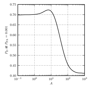
Figure 2: Detection probability at a false alarm probability of $10^{-3}$ as a function of $A$. We simulated $\sim 1.8\times 10^{7}$ signals at SNR 7 for 300 values of $A$ in the composite detection statistic defined by (20). As we expect the detection probability peaks when $A=7$, the amplitude of the signal. It is worth noting that in this case the low amplitude limit given by (21a) provides a similar detection probability. However the large signal limit given by (21b) is considerably worse.

In order to test the efficiency of the composite detection statistic versus the traditional matched filter approach we again generated $\sim 1.8\times 10^{7}$ instances of (III) for signal and signal plus noise. This time we chose a lower, more realistic, signal amplitude of $5$. The signals had uniform distributions in the template bank and in phase angle. We compare this with the standard result arising from maximizing the SNR across the bank and over phase angle

$$\rho_{\mathrm{max}}:=\mathrm{max}_{i}\left[({\bf h}\cdot{\bf s_{i(0)}})^{2}+({\bf h}\cdot{\bf s_{i(\pi/2)}})^{2}\right].$$ (26)

The result of the two procedures is shown in Fig. 3. As expected, the composite detection statistic performs worse than explicit reconstruction of the template parameters. However, when the two methods are combined, it is possible to reach the same detection probability with asymptotically low false alarm probability.

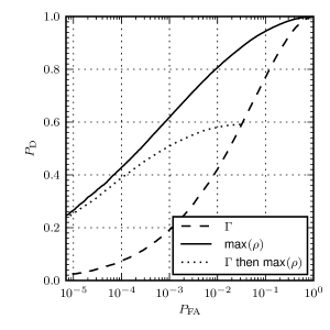
Figure 3: Receiver Operator Characteristic curves associated with different detection statistics. The solid-black trace shows the performance of choosing the maximum likelihood filter across the bank. The dashed line shows the performance of the composite detection statistic. The dotted line shows the performance of choosing max filter across the bank after conditionally thresholding on the composite detection statistic.

Fig. 3 contains three curves, showing the detection probability $P_{\mathrm{D}}$ versus false alarm probability $P_{\mathrm{FA}}$ when there is a signal with amplitude $A=5$ in the data. The solid-black line is found by choosing the maximum SNR across the filter bank as defined in (26). Maximization over the filter output is commonly done in gravitational-wave searches. The dashed-black line is the result of the composite detection statistic (20) with the choice of $A=5$. The dotted-black line is the result of first thresholding on the composite detection statistic and then conditionally maximizing the SNR over the bank. This procedure produces roughly the same detection probability for a false alarm probability of $10^{-5}$ but allows one to do the full maximization for only 3% of the filtered data.

III.2 Use example

Our simulations indicate that only $\sim 3\%$ of the data needs to have the physical template parameters reconstructed in order to have a similar detection probability as the maximum likelihood method at a false alarm probability of $10^{-5}$. This section provides an example of what this means for a realistic gravitational-wave search.

Advanced gravitational-wave detectors should be able to analyze and locate compact binary sources at the moment they merge. Prompt electromagnetic followup could confirm a gravitational-wave detection and low-latency searches will be critical to maximize the number of simultaneously observed signals. However, low-latency gravitational-wave searches will be computationally costly. The reduced filter set proposed by Cannon et al. (2010) could lower the computational cost substantially, helping to enable near real-time searches. Additionally, in this work, we have shown that it is possible to reduce the number of physical parameter reconstructions by 97% and maintain similar detection efficiencies. If these methods were to be used, it would be necessary to understand what the result in Fig. 3 implies.

We now consider how the results of Fig. (3) may apply to a low-latency gravitational-wave search and answer whether or not a false-alarm probability of $10^{-5}$ is a useful operating point. Consider the joint false alarm probability for N independent gravitational-wave detectors in coincidence

$$P_{\mathrm{FA}}=\mathcal{C}^{N-1}\times\prod_{i}^{N}P_{\mathrm{FA},i},$$ (27)

where $P_{\mathrm{FA},i}$ is the false alarm probability for the $i$th detector and $\mathcal{C}$ is the coincidence trials factor. In order to understand the double coincidence, limiting false alarm rate from the single detector false alarm probability a few pieces of information are needed. The first is the number of independent trials per second obtained by filtering the data. We will take this to be the frequency of the minimum point of the noise curve $\sim 150$ Hz. If one allows $\sim 30$ ms to define coincidence this corresponds to an additional 5 samples for coincidence trials at 150 Hz. Therefore the false alarm rate of double coincidence corresponding to a $10^{-5}$ false alarm probability in a single detector is $150\mathrm{Hz}\times 5\times 10^{-10}=7.5\times 10^{-8}\mathrm{Hz}=2.4\mathrm{yr}^{-1}$. This is well above the false rate that would be required for a detection candidate. Therefore we conclude that this procedure should not impact the detectability of near threshold signals.

IV Conclusions

We have presented a study of compact-binary gravitational-wave detection that precedes parameter estimation. This could allow more computationally efficient algorithms to be run in near real time that determine whether a signal is present before attempting to measure it’s parameters. Our study shows that it should be possible to reconstruct the physical parameters for only $\mathcal{O}[1\%]$ of the data while not impacting the sensitivity of a compact binary search.

V Acknowledgements

The authors would like to acknowledge the support of the LIGO Lab, NSF grants PHY-0653653 and PHY-0601459, and the David and Barbara Groce Fund at Caltech. LIGO was constructed by the California Institute of Technology and Massachusetts Institute of Technology with funding from the National Science Foundation and operates under cooperative agreement PHY-0757058. Research at Perimeter Institute is supported through Industry Canada and by the Province of Ontario through the Ministry of Research & Innovation. KC was supported by the National Science and Engineering Research Council, Canada. DK was supported in part from the Max Planck Gesellschaft. CH would like to thank Patrick Brady and DK would like to thank Christopher Messenger and Reinhard Prix for many fruitful discussions concerning this work. The authors would also like to thank Alan Weinstein for useful comments on this manuscript. This work has LIGO document number LIGO-P1000038-v1 and Perimeter Institute report number pi-other-203.

References

- The LIGO Scientific Collaboration (2009a) The LIGO Scientific Collaboration, Rep. Prog. Phys. 72, 076901 (2009a).
- Acernese and et al (2008) F. Acernese and et al, Classical and Quantum Gravity 25, 114045 (2008).
- Grote and the LIGO Scientific Collaboration (2010) H. Grote and the LIGO Scientific Collaboration, Classical and Quantum Gravity 27, 084003 (2010).
- The LIGO Scientific Collaboration (2009b) The LIGO Scientific Collaboration, “Advanced ligo anticipated sensitivity curves,” (2009b).
- The Virgo Scientific Collaboration (2005) The Virgo Scientific Collaboration, “Advanced virgo white paper.” (2005).
- Cutler et al. (1993) C. Cutler, T. A. Apostolatos, L. Bildsten, L. S. Finn, E. E. Flanagan, D. Kennefick, D. M. Markovic, A. Ori, E. Poisson, G. J. Sussman, and K. S. Thorne, Phys. Rev. Lett. 70, 2984 (1993).
- Kopparapu et al. (2008) R. K. Kopparapu, C. Hanna, V. Kalogera, R. O’Shaughnessy, G. González, P. R. Brady, and S. Fairhurst, The Astrophysical Journal 675, 1459 (2008).
- The LIGO Scientific Collaboration (2010) The LIGO Scientific Collaboration, Classical and Quantum Gravity 27, 173001 (2010).
- Finn and Chernoff (1993) L. S. Finn and D. F. Chernoff, Phys. Rev. D 47, 2198 (1993).
- Allen et al. (2005) B. A. Allen, W. G. Anderson, P. R. Brady, D. A. Brown, and J. D. E. Creighton, (2005), gr-qc/0509116 .
- Owen (1996) B. J. Owen, Phys. Rev. D 53, 6749 (1996).
- Cannon et al. (2010) K. Cannon, A. Chapman, C. Hanna, D. Keppel, A. C. Searle, and A. J. Weinstein, Phys. Rev. D 82, 044025 (2010).
- Wainstein and Zubakov (1962) L. A. Wainstein and V. D. Zubakov, Extraction of signals from noise (Prentice-Hall, Englewood Cliffs, NJ, 1962).
- Note (1) In practice, discretizing the parameter space is already done when choosing the initial filter bank Owen (1996).
- Anderson et al. (2001) W. G. Anderson, P. R. Brady, J. D. E. Creighton, and E. E. Flanagan, Phys. Rev. D 63, 042003 (2001).
- (16) The LIGO Scientific Collaboration, “LSC Algorithm Library,” .