The decay of turbulence generated by a class of multi-scale grids

Abstract

A new experimental investigation of decaying turbulence generated by a low-blockage space-filling fractal square grid is presented. We find agreement with previous works by Seoud & Vassilicos [“Dissipation and decay of fractal-generated turbulence”, Phys. Fluids 19, 035103 (2007)] and Mazellier & Vassilicos [“Turbulence without the Richardson-Kolmogorov cascade”, Phys. Fluids 22, 075101 (2010)] but also extend the length of the assessed decay region and consolidate the results by repeating the experiments with different probes of increased spatial resolution. It is confirmed that this moderately high Reynolds number $Re_{\lambda}$ turbulence (up to $Re_{\lambda}\simeq 350$ here) does not follow the classical high Reynolds number scaling of the dissipation rate $\varepsilon\sim u^{\prime 3}/L$ and does not obey the equivalent proportionality between the Taylor-based Reynolds number $Re_{\lambda}$ and the ratio of integral scale $L$ to Taylor micro-scale $\lambda$. Instead we observe an approximate proportionality between $L$ and $\lambda$ during decay. This non-classical behaviour is investigated by studying how the energy spectra evolve during decay and examining how well they can be described by self-preserving single-length scale forms. A detailed study of homogeneity and isotropy is also presented which reveals the presence of transverse energy transport and pressure transport in the part of the turbulence decay region where we take data (even though previous studies found mean flow and turbulence intensity profiles to be approximately homogeneous in much of the decay region). The exceptionally fast turbulence decay observed in the part of the decay region where we take data is consistent with the non-classical behaviour of the dissipation rate. Measurements with a regular square mesh grid as well as comparisons with active grid experiments by Mydlarski & Warhaft [“On the onset of high-Reynolds-number grid-generated wind tunnel turbulence”, J. Fluid Mech. vol. 320 (1996)] and Kang, Chester & Meveneau [“Decaying turbulence in an active-grid-generated flow and comparisons with large-eddy simulation”, J. Fluid Mech. vol. 480 (2003)] are also presented to highlight the similarities and differences between these turbulent flows and the turbulence generated by our fractal square grid.

1 Introduction

At high enough Reynolds numbers, the local viscous dissipation rate $\varepsilon$ of the local average turbulent kinetic energy $K$ scales with $K$ and a local correlation length scale $L$, i.e. $\varepsilon\sim K^{3/2}/L$. At least, this is what one reads in turbulence textbooks (see, for example, Batchelor, 1953; Tennekes & Lumley, 1972; Lumley, 1992; Townsend, 1956; Frisch, 1995; Lesieur, 1997; Mathieu & Scott, 2000; Pope, 2000; Sagaut & Cambon, 2008). Tennekes & Lumley (1972) introduce this scaling in their very first chapter with the words “it is one of the cornerstone assumptions of turbulence theory”. Townsend (1956) uses it explicitly in his treatment of free turbulent shear flows (see page 197 in Townsend, 1956) which includes wakes, jets, shear layers, etc. Since G.I Taylor introduced it in 1935 Taylor (1935), this scaling is also customarily used in theories of decaying homogeneous isotropic turbulence (see Batchelor, 1953; Frisch, 1995; Rotta, 1972) and in analyses of wind tunnel simulations of such turbulence (e.g. Batchelor & Townsend, 1948; Comte-Bellot & Corrsin, 1966) in the form

$$\varepsilon=C_{\varepsilon}\frac{u^{\prime 3}}{L}$$ (1)

where $u^{\prime}$ is the r.m.s. velocity fluctuation, $L$ is an integral length scale and $C_{\varepsilon}$ is a constant independent of time, space and Reynolds number when the Reynolds number is large enough. However, as Taylor (1935) was careful to note, the constant $C_{\varepsilon}$ does not need to be the same irrespective of the boundaries (initial conditions) where the turbulence is produced (see Burattini, Lavoie & Antonia, 2005; Mazellier & Vassilicos, 2008; Goto & Vassilicos, 2009).

In high Reynolds number self-preserving free turbulent shear flows, the cornerstone scaling $\varepsilon\sim K^{3/2}/L$ determines the entire dependence of $\varepsilon$ on the streamwise coordinate and ascertains its independence on Reynolds number (see Townsend, 1956). This cornerstone scaling is also effectively used in turbulence models such as $K-\varepsilon$ (see Pope, 2000) and in Large Eddy Simulations (see Lesieur, 1997; Pope, 2000). The assumption that $\varepsilon$ is independent of Reynolds number when the Reynolds number is large enough is an inseparable part of the Richardson-Kolmogorov cascade Tennekes & Lumley (1972); Frisch (1995). This is the celebrated nonlinear dissipation mechanism of the turbulence whereby, within a finite time $L/\sqrt{K}$ (the same time scale for all high enough Reynolds numbers), smaller and smaller “eddies” are generated till eddies so small are formed which can very quickly lose their kinetic energy by linear viscous dissipation. The higher the Reynolds number, the smaller the size of these necessary dissipative eddies but the time scale $L/\sqrt{K}$ for energy to cascade to them from the large eddies remains the same. The dissipation rate $\varepsilon$ is proportional to $K$ divided by this time, and therefore $\varepsilon\sim K^{3/2}/L$.

In various high Reynolds number self-preserving free turbulent shear flows as in wind tunnel grid-generated turbulence, $K$ and $L$ vary with streamwise downstream distance $x-x_{0}$ (where $x_{0}$ is an effective/virtual origin) as power laws. Specifically, $K\sim U_{\infty}^{2}({x-x_{0}\over L_{B}})^{-n}$ and $L\sim L_{B}({x-x_{0}\over L_{B}})^{m}$ where $L_{B}$ is a length-scale characterising the inlet and $U_{\infty}$ is the appropriate inlet velocity scale. In table 1 we recall the generally accepted values taken by the exponents $n$ and $m$ in plane wakes, axisymmetric wakes, self-propelled plane wakes, self-propelled axisymmetric wakes, mixing layers, plane jets, axisymmetric jets and wind-tunnel grid-generated turbulence (from Tennekes & Lumley, 1972; Comte-Bellot & Corrsin, 1966). Estimating a Taylor microscale $\lambda$ from $\varepsilon\sim\nu K/\lambda^{2}$ where $\nu$ is the kinematic viscosity of the fluid, and then applying the cornerstone assumption $\varepsilon\sim K^{3/2}/L$ to all these flows yields the following two relations:

$$L/\lambda\sim Re_{0}^{1/2}({x-x_{0}\over L_{B}})^{{m\over 2}-{n\over 4}}$$ (2)

and

$$\sqrt{K}\lambda/\nu\sim Re_{0}^{1/2}({x-x_{0}\over L_{B}})^{{m\over 2}-{n\over 4}}$$ (3)

where $Re_{0}\equiv U_{\infty}L_{B}/\nu$ is the inlet Reynolds number and $\sqrt{K}\lambda/\nu$ is a local Taylor microscale-based Reynolds number. The different values of ${m\over 2}-{n\over 4}$ are given in table 1. Remarkably, $\varepsilon\sim K^{3/2}/L$ implies that $L/\lambda\sim\sqrt{K}\lambda/\nu$ in all these flows whatever the values of $n$ and $m$, meaning that $L/\lambda\sim\sqrt{K}\lambda/\nu$ collapses the $Re_{0}$ and the $x$ dependencies in the same way for all these flows. We stress that this collapse is the immediate consequence of $\varepsilon\sim K^{3/2}/L$. The relation $L/\lambda\sim\sqrt{K}\lambda/\nu$ simply reflects the Richardson-Kolmogorov cascade: the higher the Reynolds number, the smaller the size of the dissipative eddies, i.e. the greater the range of excited scales and the greater $L/\lambda$.

As noted by Lumley (1992), by 1992 there had not been too much detailed and comprehensive questioning of data to establish the validity of $\varepsilon\sim K^{3/2}/L$ but he wrote: “I hardly think the matter is really much in question”. He cited the data compilations of Sreenivasan (1984) which suggested that $C_{\varepsilon}$ does become constant at $Re_{\lambda}=u^{\prime}\lambda/\nu$ larger than about 50 for wind tunnel turbulence generated by various biplane square-mesh grids, but there seemed to be little else at the time. Since then, direct numerical simulations (DNS) of high Reynolds number statistically stationary homogeneous isotropic turbulence have significantly strengthened support for the constancy of $C_{\varepsilon}$ at $Re_{\lambda}$ greater than about 150 (see compilation of data in Burattini et al. (2005), see also Sreenivasan (1998)). Other turbulent flows have also been tried in the past fifteen years or so such as various turbulent wakes and jets and wind tunnel turbulence generated by active grids (see Burattini et al., 2005; Mazellier & Vassilicos, 2008) with some, perhaps less clear, support of the constancy of $C_{\varepsilon}$ at large enough $Re_{\lambda}$ (perhaps larger than about 200 if $L$ is defined appropriately, see Burattini et al. (2005)) and also some clear indications that the high Reynolds number constant value of $C_{\varepsilon}$ is not universal, as indeed cautioned by Taylor (1935).

Table 1: Powers law exponents characteristic of the downstream evolutions of $K$, $L$, $L/\lambda$

	$K$	$L$	$L/\lambda$
Plane wake	1	1/2	0
Axisymmetric wake	4/3	1/3	-1/6
Self-propelled plane wake	3/2	1/4	-1/4
Self-propelled axisymmetric wake	8/5	1/5	-3/10
Mixing layer	0	1	1/2
Plane jet	1	1	1/4
Axisymmetric jet	2	1	0
Regular grid turbulence	1.25	0.35	-0.14

A decade ago, Queiros-Conde & Vassilicos (2001) took the opposite approach and asked whether it might be possible to break $\varepsilon\sim K^{3/2}/L$ in some fundamental way in some flows, and so they proposed generating turbulence with fractal/multiscale objects/stirrers/inlet conditions. Some years later, Hurst & Vassilicos (2007) published an exploratory study of wind tunnel grid-generated turbulence where they tried twenty one different planar grids from three different families of passive fractal/multiscale grids: fractal cross grids, fractal I grids and fractal square grids. They ascertained that the fractal dimension $D_{f}$ of these grids needs to take the maximal value $D_{f}=2$ for least downstream turbulence inhomogeneity. They also identified some important grid-defining parameters (such as the thickness ratio $t_{r}$, see figure 1 and table 3) and some of their effects on the flow, in particular on the Reynolds number $Re_{\lambda}$ which they showed can reach high values with some of these grids in small and conventional sized wind tunnels, comparable to values of $Re_{\lambda}$ achieved with active grids in similar wind tunnels and wind speeds. Their most interesting, and in fact intriguing, results were for their space-filling ($D_{f}=2$) low-blockage (25%) fractal square grids (see figure 1). Fractal square grids have therefore been the multiscale grids of choice in most subsequent works on multiscale/fractal-generated turbulence Seoud & Vassilicos (2007); Nagata, Suzuki, Sakai, Hayase & Kubo (2008b, a); Stresing, Peinke, Seoud & Vassilicos (2010); Mazellier & Vassilicos (2010); Suzuki, Nagata, Sakai & Ukai (2010); Laizet & Vassilicos (2011). For the case of space-filling low-blockage fractal square grids, Hurst & Vassilicos (2007) found a protracted region between the grid and a distance $x_{peak}$ downstream of the grid where the turbulence progressively builds up; and a decay region region at $x>x_{peak}$ where the turbulence continuously decays downstream. They reported a very fast turbulence decay which they fitted with an exponential and also reported very slow downstream growths of the longitudinal and lateral integral length-scales and of the Taylor microscale. (Very recently, Krogstad & Davidson (2011) studied the decay behind multiscale cross grids and found conventional decay rates. Note that for multiscale cross grids our prior publications did not claim fast, unconventional, decay rates Hurst & Vassilicos (2007). This may serve as further justification for focusing attention on fractal square grids in the present paper. Even so, multiscale cross grids have been used successfully in some recent studies for enhancing the Reynolds number, see Kinzel, Wolf, Holzner, Lüthi, Tropea & Kinzelbach (2011) and Geipel, Henry Goh & Lindstedt (2010).)

Seoud & Vassilicos (2007) concentrated their attention on the decay region of turbulence generated by space-filling low-blockage fractal square grids and confirmed the results of Hurst & Vassilicos (2007). In particular, they showed that $L/\lambda$ remains approximately constant whilst $Re_{\lambda}$ decays with downstream distance $x$ and they noted that this behaviour implies a fundamental break from (1) where $C_{\varepsilon}$ is constant. They also found that one-dimensional longitudinal energy spectra at different downstream centreline locations $x$ can be made to collapse with $u^{\prime}$ and a single length-scale, as opposed to the two length-scales ($L$ and Kolmogorov microscale) required by Richardson-Kolmogorov phenomenology. Finally, they also carried out homogeneity assessments in terms of various profiles (mean flow, turbulence intensity, turbulence production rate) as well as some isotropy assessments.

Mazellier & Vassilicos (2010) also worked on wind tunnel turbulence generated by space-filling low-blockage fractal square grids. They introduced the wake-interaction length-scale $x_{*}$ which is defined in terms of the largest length and thickness on the grid and they showed from their data that $x_{peak}\approx 0.5x_{*}$. They documented how very inhomogeneous and non-Gaussian the turbulent velocity statistics are in the production region near the grid and how homogeneous and Gaussian they appear by comparison beyond $0.5x_{*}$. They confirmed the findings of Hurst & Vassilicos (2007) and Seoud & Vassilicos (2007) and added the observation that both $Re_{\lambda}$ and $L/\lambda$ are increasing functions of the inlet velocity $U_{\infty}$. Thus, the value of $L/\lambda$ seems to be set by the inlet Reynolds number, in this case defined as $Re_{0}=U_{\infty}x_{*}/\nu$ for example.

Finally, Mazellier & Vassilicos (2010) brought the two different single-scale turbulence decay behaviours of George (1992) and George & Wang (2009) into a single framework which they used to analyse the turbulence decay in the downstream region beyond $x_{peak}\approx 0.5x_{*}$. This allowed them to introduce and confirm against their data the notions that, in the decay region, the fast turbulence decay observed by Hurst & Vassilicos (2007) and Seoud & Vassilicos (2007) may not be exponential but a fast decaying power-law and that $L$ and $\lambda$ are in fact increasing functions of $x$ which keep $L/\lambda$ approximately constant.

The results of Hurst & Vassilicos (2007), Seoud & Vassilicos (2007) and Mazellier & Vassilicos (2010) suggest that, in the decay region downstream of space-filling low-blockage fractal square grids, high Reynolds number turbulence is such that

$$L/\lambda\sim Re_{0}^{\alpha}A({x-x_{0}\over x_{*}})$$ (4)

and

$$Re_{\lambda}\sim Re_{0}^{\beta}B({x-x_{0}\over x_{*}})$$ (5)

where $A$ is a slow-varying dimensionless function of ${x-x_{0}\over x_{*}}$ (in fact effectively constant), $B$ is a fast-decreasing dimensionless function of ${x-x_{0}\over x_{*}}$ (perhaps even as fast as exponential), and $\alpha$ and $\beta$ are positive real numbers.

Assuming that the dissipation-scale turbulence structure is approximately isotropic, we now use the relation $\varepsilon=15\nu u^{\prime 2}/\lambda^{2}$ which Taylor (1935) obtained for isotropic turbulence. With (1) this relation implies

$$\frac{L}{\lambda}=\frac{C_{\varepsilon}}{15}Re_{\lambda}$$ (6)

and, clearly, $C_{\varepsilon}$ cannot be constant (independent of $Re_{0}$ and $x$) with $Re_{0}$ and $x$ dependencies of $L/\lambda$ and $Re_{\lambda}$ such as those observed in wind tunnel turbulence generated by space-filling low-blockage fractal square grids. Instead,

$$C_{\varepsilon}=15Re_{0}^{\alpha-\beta}A({x-x_{0}\over x_{*}})/B({x-x_{0}\over x_{*}})$$ (7)

which means that $C_{\varepsilon}$ should be increasing fast in the downstream direction but which also means that a plot of $C_{\varepsilon}$ versus $Re_{\lambda}$ can be quite different depending on whether $Re_{\lambda}$ is varied by varying $Re_{0}$ whilst staying at the same position $x$ or by moving along $x$ whilst keeping $Re_{0}$ constant. This is a point which we discuss and attempt to bring out clearly in the present paper.

Relations (4) and (5) and their consequent decoupling of $L/\lambda$ and $Re_{\lambda}$ were observed at moderate to high values of $Re_{\lambda}$ where Seoud & Vassilicos (2007) and Mazellier & Vassilicos (2010) also observed a well-defined broad power-law energy spectrum. Indeed $Re_{\lambda}$ needs to be large enough for the study of fully developed turbulence. Active grids were introduced by Makita (1991) to improve on the Reynolds number values achieved by regular grids in conventional wind tunnels. Fractal square grids achieve comparably high values of $Re_{\lambda}$ but also a far wider range of $Re_{\lambda}$ values along the streamwise direction. This makes if much easier to study $Re_{\lambda}$-dependencies, a point which we make and discuss in some detail in the present paper.

In this paper we report an experimental assessment of turbulent flows generated by a low-blockage space-filling fractal square grid (see figure 1) and a regular square-mesh grid. The main focus of this paper is to complement former research on fractal-generated turbulence by extending the assessed decay region and using the new data to re-address the previously reported dramatic departure from $C_{\varepsilon}=Const$ and $A({x-x_{0}\over x_{*}})=B({x-x_{0}\over x_{*}})$ and the abnormally high decay exponents Hurst & Vassilicos (2007); Seoud & Vassilicos (2007); Mazellier & Vassilicos (2010). We provide estimates of these exponents, and also show that $\alpha\approx\beta$ and that our fractal-generated turbulence behaves in a way which is very close to self-preserving single-length scale turbulence Mazellier & Vassilicos (2010), particularly if the turbulence anisotropy is taken into account when calculating 3D energy spectra. We also show that, even though previous studies by Seoud & Vassilicos (2007) and Mazellier & Vassilicos (2010) found that the mean flow and turbulence profiles are approximately homogeneous in much of the decay region, there nevertheless remains significant transverse turbulent transport of turbulent kinetic energy and turbulent transport of pressure. The decaying turbulence is therefore not homogeneous and isotropic in terms of third order one point statistics even though it more closely is in terms of lower order one point statistics. Whenever possible a comparison between fractal-generated and non-fractal-generated turbulence is made emphasising similarities and differences.

In the following section we describe the experimental apparatus as well as the anemometry systems, probes and the details of the data acquisition. The experimental results are presented in Sec. 3 and are organised in four subsections. In Sec. 3.1 it is suggested that the wake-interaction length-scale introduced by Mazellier & Vassilicos (2010) to characterise the extent of the production region in the lee of the fractal grid is also meaningful for regular static grids. In Sect. 3.2 the homogeneity and isotropy of the fractal-generated flow is investigated following the methodology used by Corrsin (1963) and Comte-Bellot & Corrsin (1966) for regular static grids. In Sec. 3.3 & 3.4 the normalised energy dissipation rate and the decay law are re-assessed using the new data. In Sec. 3.5 we investigate the possibility of a self-similar, single-length-scale behaviour by collapsing the 1D energy spectra and the $2^{nd}$-order structure functions using large-scale variables; also the 3D energy spectrum function is calculated to provide isotropy corrections on the collapse. In Sec. 4 we end this paper by highlighting the main conclusions drawn from the present measurements and discuss some of the questions raised.

2 The experimental setup

2.1 Experimental hardware

The experiments are performed in the $T=0.46m$ wind-tunnel described in some detail in Mazellier & Vassilicos (2010) and sketched in figure 5 ($T$ is the lateral width of the tunnel’s square test section). The inlet velocity $U_{\infty}$ is imposed and stabilised with a PID feedback controller using the static pressure difference across the 8:1 contraction and the temperature near the inlet of the test section which are measured using a Furness Controls micromanometer FCO510.

All data are taken with one- and two-component hot-wire anemometers operating in constant-temperature mode (CTA). The hot-wires are driven by a DANTEC StreamLine CTA system with an in-built signal conditioner. We use both square- and sine-wave testing to measure the cut-off frequency at the verge of attenuation ($f^{0dB}_{cut-off}$) and at the standard ’-3dB’ attenuation level ($f^{-3dB}_{cut-off}$). In table 2 we present the results from the electronic testing of our anemometry system. Further information concerning electronic testing of thermal anemometers and a discussion of the consistency between the square and sine-wave tests can be found in Freymuth (1977).

For the single component measurements three different single-wires (SW) are used with a sensing length ($l_{w}$) of $1mm$, $0.45mm$ & $0.2mm$ respectively. For the two component measurements two cross-wires (XW) with sensing lengths of $l_{w}=0.5$ & $1mm$ respectively are used, but for both the separation between the wires is around $1mm$. All the sensors except the $l_{w}=1mm$ XW are based on Dantec probes modified to use in-house etched Platinum-(10%)Rhodium Wollaston wires soldered to the prongs (further details can be found in table 2). The $l_{w}=1mm$ XW is a Dantec 55P51 tungsten probe. It should be noted that the $l_{w}=0.2mm$ single-wire, which has a diameter of $d_{w}=1.27\mu m$, is operated in the limit of the bridge stability, on the verge of having non-damped oscillations. Nonetheless, the sine-wave test indicated that $f^{0dB}_{\mathrm{cut-off}}$ was about $40kHz$. The hot-wires are calibrated at the beginning and at the end of each measurement campaign using a $4^{th}$-order polynomial in the SW case and a velocity-pitch map in the XW case. Note that, unless otherwise stated, the data shown are acquired with the $l_{w}\approx 1mm$ SW hot-wire probe. All the two-component data presented are acquired with the $l_{w}\approx 0.5mm$ XW except the spanwise traverse data presented in Sec. 3.2.1.

Note that two other anemometry systems have been used as well in order to compare with previous experimental results, but these results are not included here. The other anemometry systems are: the AALab AN-1005 CTA system used in Seoud & Vassilicos (2007) and Hurst & Vassilicos (2007) and the DISA 55M10 CTA bridge with a DISA 55D26 signal conditioner used in Mazellier & Vassilicos (2010). It is found that the results obtained with the DISA 55M10 CTA unit closely match those obtained with the StreamLine CTA system, when the same hot-wire probe is used, except at very high frequencies where the higher noise floor of the DISA CTA system buries the velocity signal. On the other hand it is found that the measurements taken with the AALab AN-1005 CTA system are significantly different at frequencies above $6$kHz and therefore the turbulence statistics involving velocity derivatives are significantly different. This is likely the reason for the difference between the normalised energy dissipation rate $C_{\varepsilon}$ results reported in Seoud & Vassilicos (2007) and the ones presented in Sec. 3.3 of this paper. The comparison between the results of the different anemometry systems will be presented elsewhere.

SW/XW	$l_{w}$	$d_{w}$	$l_{w}/d_{w}$	Hot-wire	$U_{\infty}$	$f^{-3dB}_{\mathrm{cut-off}}$	$f^{0dB}_{\mathrm{cut-off}}$	$l_{w}/\eta$
	$(mm)$	$(\mu m)$		probe	$(ms^{-1})$	$(kHz)$	$(kHz)$
SW	$\sim 1$	$5.1$	$196$	55P16	10	$\sim 25$	$\sim 12$	7-3
					15	$\sim 32$	$\sim 16$	9-5
SW	$\sim 0.45$	$2.5$	$180$	55P16	10	$\sim 45$	$\sim 21$	3-2
					15	$\sim 45$	$\sim 23$	4-2
SW	$\sim 0.2$	$1.27$	$157$	55P11	10	$>50$	$\sim 40$	$\sim 1$
					15	$>50$	$\sim 40$	2-1
XW	$\sim 0.5$	$2.5$	$200$	55P51	10	$\sim 45$	$\sim 21$	3-2
					15	$\sim 45$	$\sim 23$	4-2
XW	$1.0$	$5$	$200$	55P51	15	$\sim 30$	$\sim 14$	9-5

Table 2: Details on the hot-wires, cut-off frequencies & resolution. $l_{w}$ and $d_{w}$ are the sensing length and diameter of the wires, $l_{w}/\eta$ is the ratio between the sensing length and the Kolmogorov inner length-scale and $U_{\infty}$ is the inlet velocity. $f^{-3dB}_{\mathrm{cut-off}}$ is the cut-off frequency corresponding to $-3dB$ signal attenuation and $f^{0dB}_{\mathrm{cut-off}}$ is the highest frequency with negligible attenuation.

2.2 Data acquisition and signal processing

The pressure and temperature measurements are digitally transferred to the computer using a parallel port. The analogue signal from the anemometers is sampled using a 16-Bit National Instruments NI-6229(USB) card, at a sampling frequency set to be higher than twice the analogue low-pass filtering frequency ($30$kHz). The data acquisition and signal processing are performed with the commercial software MATLAB^TM.

The turbulent velocity signal was acquired for 9min corresponding to more than 100,000 integral-time scales. This was confirmed to be sufficient for converged measured statistics of interest such as the integral scale, the first four moments of the velocity signal and the 2^nd moment of the velocity derivative signal. The time-varying turbulent signal was converted into spatially-varying by means of a local Taylor’s hypothesis following the algorithm proposed in Kahalerras et al. (1998). Before Taylor’s hypothesis is used the signal is digitally filtered at a frequency corresponding to $k_{1}\eta\sim 1.1$ (where $\eta\equiv(\nu^{3}/\varepsilon)^{1/4}$ is the Kolmogorov inner length-scale and $k_{1}$ the wavenumber) using a $4^{th}$-order Butterworth filter to eliminate higher frequency noise.

The integral scale $L_{u}$ is estimated as

$$L_{u}=\int_{0}^{r_{L}}f(r)\,dr,$$

where $f(r)\equiv\overline{u(x)u(x+r)}/\overline{u(x)^{2}}$ is the auto-correlation function of the streamwise velocity fluctuations for streamwise separations $r$ and $r_{L}$ is maximum integration range taken to be about $10$ times the integral length scale. It was checked that (i) changing the integration limit $r_{L}$ by a factor between $2/3$ and $2$ has little effect on the numerical value of the integral scale and (ii) the choice of $r_{L}$, if large enough, does not influence the way that $L_{u}$ varies with downstream distance. The transverse integral scale is estimated in a similar way. The longitudinal and transverse spectra are calculated using an FFT based periodogram algorithm using a Hanning window with 50% overlap and window length equivalent to at least $180$ integral length scales. The dissipation $\varepsilon$ is estimated from the longitudinal wavenumber spectra $F_{11}$ as

$$\varepsilon=15\nu\int_{k_{min}}^{k_{max}}k_{1}^{2}\,F_{11}(k_{1})\,dk_{1},$$

where $k_{min}$ and $k_{max}$ are determined by the window length and the sampling frequency respectively. To reduce the unavoidable contamination of noise at high frequencies (which can bias the dissipation estimate) we follow Antonia (2003) and fit an exponential curve to the high frequency end of the spectra which we then integrate. We checked that calculating the dissipation with and without Antonia’s (2003) method changes the dissipation by less than $4\%$ in the worst case.

It might be worth mentioning that the measurements of the fractal grid-generated turbulence posed a lesser challenge to hot-wire anemometry than the regular grid-generated turbulence quite simply because the turbulent signal to anemometry noise ratio is higher in the former case, but nonetheless the Kolmogorov microscales (which influence the maximum frequency to be measured) for the highest $Re_{\lambda}$ measurement location ($Re_{\lambda}\approx 350$ and $Re_{\lambda}\approx 150$ respectively) are roughly the same ($\eta\approx 0.11mm$ and $\eta\approx 0.13mm$ respectively).

2.3 Turbulence generating grids

The bulk part of the measurements are performed on turbulence generated by a low-blockage space-filling fractal square grid (SFG) with 4 ’fractal iterations’ and a thickness ratio of $t_{r}=17$, see figure 1. It is one of the grids used in the experimental setup of Mazellier & Vassilicos (2010) where further details of the fractal grids and their design can be found. Measurements of turbulence generated by a regular bi-plane grid (RG) with a square mesh and composed of square rods are also performed. The summary of the relevant grid design parameters is given in table 3.

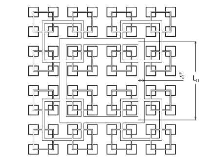
Figure 1: Low-blockage space-filling fractal square grid (SFG). The grid is space-filling because the fractal dimension of its delimiting line takes the maximum value of $2$ over the range of scales on the grid. In the limit of infinite number of fractal iterations the blockage ratio will tend to unity, without taking bar thickness into account. However with only four iterations and the bar thickness in the figure the grid’s blockage ratio is only 25%.

Grid	N	$L_{0}$	$t_{0}$	$L_{r}$	$t_{r}$	$R_{L}$	$R_{t}$	$\sigma$	$M_{eff}$
		$(mm)$	$(mm)$						$(mm)$
SFG	4	237.8	19.2	8	17	0.5	2.57	0.25	26.2
RG	1	60	10	1	1	1	1	0.32	60

Table 3: Details of the regular grid (RG) and the low-blockage space-filling fractal square grid (SFG). $N$ is the number of fractal iterations of the grids (for a regular grid $N=1$). $L_{0}$ is the centreline distance separating the largest bars and $t_{0}$ their lateral thickness, see figure 1. $L_{r}$ and $t_{r}$ are respectively the length and thickness ratio between the largest and smallest bars. $R_{L}$ and $R_{t}$ are the length and thickness ratio between two consecutive fractal iterations. $R_{t}$ is related to $t_{r}$ and $N$ via $t_{r}=R_{t}^{-N+1}$. The blockage ratio $\sigma$ is defined as the fraction of area occupied by the grid and $M_{eff}$ is the effective mesh size as defined in Hurst & Vassilicos (2007) which reverts to the definition of mesh size for a regular grid.

3 Results

The turbulent field in the lee of the space-filling fractal square grids can be considered to have two distinct regions Hurst & Vassilicos (2007); Mazellier & Vassilicos (2010): a production region where the turbulent kinetic energy (on the centreline) is increasing and the flow is being homogenised, and a decay region where the energy of the turbulent fluctuations are rapidly decreasing and the flow is roughly homogeneous with an isotropy factor around $u^{\prime}/v^{\prime}\sim 1.1-1.25$, where $u^{\prime}$ and $v^{\prime}$ are the longitudinal and transverse r.m.s. velocities respectively.

3.1 The wake-interaction length-scale

Mazellier & Vassilicos (2010) introduced the wake-interaction length-scale $x_{*}=L_{0}^{2}/t_{0}$ (see definitions of $L_{0}$ & $t_{0}$ in figure 1 and in the caption of table 3) to characterise the extent of the turbulence production region in the lee of the space-filling fractal square grids. This length-scale is based on the largest square of the grid since the wakes it generates are the last to interact, although there is a characteristic wake-interaction length-scale for each grid iteration (for a schematic of the wake interactions occurring at different streamwise locations refer to figure 4a in Mazellier & Vassilicos, 2010). They then related the wake interaction length-scale with the location of the maximum of the turbulence intensity along the centreline $x_{peak}$, which marks the end of the production region and the start of the decay region and found that $x_{peak}/x_{*}\approx 0.45$. Note that this is not the only peak in turbulence intensity in the domain nor is it the overall maximum, but it is the last peak occurring furthest downstream before decay. This can be seen for example in figure 9 in Mazellier & Vassilicos (2010), where the streamwise variations of the turbulence intensity both along the centreline and along an off-centre parallel line are shown. The turbulence intensity along this particular off-centre line peaks much closer to the grid and at a higher intensity value than the turbulence recorded on the centreline.

The wake-interaction length-scale can also be defined for a regular grid, where the mesh size and the bar thickness are now the relevant parameters, $x_{*}=M^{2}/t_{0}$. Jayesh & Warhaft (1992) measured the turbulence intensity very near the grid, $1<x/M<30$ and observed two different regions, a highly inhomogeneous region up to $x/M\approx 3$ which is a production region where the turbulence intensity increases along a streamwise line crossing half distance between grid bars and a decay region beyond that. Note that $x/M\approx 3$ corresponds to $x_{peak}/x_{*}\approx 0.55$ close to $x_{peak}/x_{*}\approx 0.45$ encountered by Mazellier & Vassilicos (2010) for the fractal square grids. A qualitatively similar conclusion can be drawn from the direct numerical simulation of turbulence generated by a regular grid presented in Ertunç, Özyilmaz, Lienhart, Durst & Beronov (2010). In their figure 16 one can find the development of the turbulent kinetic energy very close to the grid $0.5<x/M<10$ along three straight streamwise lines located, respectively, behind a grid bar, half-distance between bars and in-between the other two traverses. It can be seen that the turbulence intensity peaks first directly behind the grid bar at $x_{peak}/M\approx 1$ and lastly behind the half-distance between grid bars (somewhat equivalent to the centreline in the square fractal grid) at $x_{peak}/M\approx 2.5$. This latter streamwise location corresponds to $x_{peak}/x_{*}\approx 0.68$, once more not far from $x_{peak}/x_{*}\approx 0.45$. Note nonetheless that this simulation was performed at very low Reynolds numbers, $Re_{\lambda}<17$, so care must be taken in quantitative comparisons.

Note that $x_{peak}/x_{*}$ appears to be slightly higher for the regular static grids than for the fractal square grids. This is likely due not only to the typically low Reynolds numbers generated by the regular grids but also to the characteristic production mechanism of the fractal square grids, i.e. before the larger wakes interact all the smaller wakes have already interacted and generated turbulence that increases the growth rate of the larger wakes, thus making them meet closer to the grid and therefore causing a smaller value of $x_{peak}/x_{*}$.

The fact that the fractal grid has multiple wake-interaction length-scales, for the present fractal square grid ranging from a few centimetres to more than a meter, is precisely part of what makes the fractal grid generate turbulence that is qualitatively different from regular grid-generated turbulence. Consequently one could expect that a fractal grid designed so that it produces a narrow range or a single dominant wake-interaction length-scale, will lead to turbulence that is similar to regular grid-generated turbulence. Hurst & Vassilicos (2007) included in their study the assessment of fractal cross grids, which resemble regular grids but with bars of varying thicknesses. The ratios between the thickest and the thinnest bars of their fractal cross grids ranged from 2.0 to 3.3, thus yielding a narrow span of wake-interaction length-scales. Furthermore, the wake interaction pattern of the fractal cross grids, as designed and studied in Hurst & Vassilicos (2007), is considerably different from the wake interaction pattern of their fractal square grids. In the fractal square grids case, the main interaction events occur when similar sized wakes meet, whereas in the fractal cross grids the main interaction events occur between adjacent wakes, which may or may not be of similar size. Therefore one could expect the results obtained with fractal cross grids, for example the power-law turbulence decay exponent, not to be very different from the typical results found for regular grid-generated turbulence. In fact, examining figure 10 in Hurst & Vassilicos (2007) one can see that the turbulence decays as $(x-x_{0})^{-n}$ with $1<n<1.5$ for $x_{0}\approx 0$, although they encounter a general difficulty of finding the appropriate virtual origin. We will return to the problem of finding the appropriate virtual origin and the power-law decay exponent in Sec. 3.4 where we present different power-law decay fitting methods applied to our data.

3.2 Homogeneity, isotropy and wall interference

3.2.1 Homogeneity

Previous experimental investigations on the turbulence generated by space-filling fractal square grids, e.g. Mazellier & Vassilicos (2010), reported that the flow field close to the grid is highly inhomogeneous. It was also observed that during the process of turbulent kinetic energy build up the turbulent flow is simultaneously homogenised by turbulent diffusion, and by the time it reaches a peak in turbulence intensity (what they considered to be the threshold between the production and decay regions) the flow has smoothed out most inhomogeneities. Seoud & Vassilicos (2007) measured the turbulent kinetic energy production in various planes perpendicular to the mean flow along the centreline and observed that the turbulent production decreases rapidly just after the peak, i.e. where $0.45(\approx x_{peak}/x_{*})<x/x_{*}<0.75$ and that the turbulent energy production typically represents less than $30\%$ of the dissipation and never exceeds $20\%$ beyond this region.

Mazellier & Vassilicos (2010) compared the characteristic time scales of the mean velocity gradients $({\partial U\over\partial x})^{-1}$ and $({\partial U\over\partial y})^{-1}$ (where $U$ is the streamwise mean velocity and $y$ is a coordinate along the horizontal normal to the streamwise direction) with the time scale associated with the energy-containing eddies and reached the conclusion that beyond the peak the mean gradient time scale is typically one to two orders of magnitude larger. Consequently the small-scale turbulence dynamics are not affected by large-scale mean flow inhomogeneities.

Here we complement the previous analyses by following the approach of Corrsin (1963) and Comte-Bellot & Corrsin (1966) and using some of their homogeneity criteria, as they did for regular grids. The commonly accepted ’rule-of-thumb’ for the regular grids is that the turbulent flow can be considered statistically homogeneous in transverse planes for $x/M>30$ and the unavoidable inhomogeneity along the mean flow direction becomes relatively unimportant for $x/M>40$ Corrsin (1963).

For the downstream decaying turbulence to be considered a good approximation to spatially homogeneous decaying turbulence two criteria must be met, (i) the eddy turn-over time $L_{u}/u^{\prime}$ must be small compared to the time-scale associated with the velocity fluctuation decay rate $(\partial u^{\prime}/\partial x)^{-1}$ (see also Sec. 3.3 of Townsend, 1956) and (ii) the rate of change of the turbulent length-scales must be small compared to the length-scales themselves. Following Corrsin (1963) we measure

$$\frac{L_{u}}{\overline{u^{2}}}\frac{\partial\overline{u^{2}}}{\partial x},\hskip 5.69054pt\frac{L_{u}}{\lambda}\frac{\partial\lambda}{\partial x},\hskip 5.69054pt\frac{\partial L_{u}}{\partial x},$$

and confirm that these quantities are small for the entire decay region assessed here, i.e $x/x_{*}>0.6$ (figure 2a) and comparable with those obtained for a regular grid (figure 2b). Note that the ’rule-of-thumb’ $x/M>40$ suggested by Corrsin (1963) was based on the streamwise location where his regular grid data yielded these dimensionless quantities to be below 4%, so for our regular grid data this ’rule-of-thumb’ translates to $x/M>25$ and for our fractal square grid data to $x/x_{*}>0.7$.

A thorough assessment of the inhomogeneity of the flow can be made by using the statistical equations and measuring the terms that should be zero in a statistically homogeneous flow field. Starting with single-point statistics, e.g. the turbulent kinetic energy equation (here $U_{1}=U$, $U_{2}=V$ & $U_{3}=W$ denote mean flow speeds, $u_{1}=u$, $u_{2}=v$, $u_{3}=w$ & $p$ are zero mean fluctuating velocities and pressure, and $x_{1}=x$, $x_{2}=y$ & $x_{3}=z$ are the components of a coordinate system aligned with the respective velocity components),

$$\frac{U_{k}}{2}\frac{\partial\,\overline{q^{2}}}{\partial x_{k}}=-\overline{u_{i}u_{j}}\,\frac{\partial U_{i}}{\partial x_{j}}-\frac{\partial}{\partial x_{k}}\left(\frac{\overline{u_{k}q^{2}}}{2}+\frac{\overline{u_{k}p}}{\rho}\right)+\frac{\nu}{2}\frac{\partial^{2}\overline{q^{2}}}{\partial x_{m}\partial x_{m}}-\nu\overline{\frac{\partial u_{i}}{\partial x_{k}}\frac{\partial u_{i}}{\partial x_{k}}},$$ (8)

where use is made of Einstein’s notation and $\overline{q^{2}}\equiv\overline{u^{2}}+\overline{v^{2}}+\overline{w^{2}}$ ($K\equiv{1\over 2}\overline{q^{2}}$), over-bars signifying averages over an infinite number of realisations (here, over time).

The flow statistics inherit the grid symmetries, i.e. reflection symmetry around the y & z axes (as well as diagonal reflection symmetry) and symmetry with respect to discrete $90^{\circ}$ rotations and therefore the transverse mean velocities are negligibly small, $V=W\approx 0$, and the turbulent kinetic energy equation at the centreline reduces to:

$$\frac{U}{2}\frac{\partial\,\overline{q^{2}}}{\partial x}=\overbrace{-\left(\overline{u^{2}}\,\frac{\partial U}{\partial x}+2\overline{uv}\,\frac{\partial U}{\partial y}\right)}^{\mathcal{P}} \overbrace{-\left(\frac{\partial}{\partial x}\frac{\overline{uq^{2}}}{2}+2\frac{\partial}{\partial y}\frac{\overline{vq^{2}}}{2}\right)}^{\mathcal{T}}$$ (9)

$$\underbrace{-\left(\frac{\partial}{\partial x}\frac{\overline{up}}{\rho}+2\frac{\partial}{\partial y}\frac{\overline{vp}}{\rho}\right)}_{\Pi} \underbrace{+\frac{\nu}{2}\left(\frac{\partial^{2}\overline{q^{2}}}{\partial x^{2}}+2\frac{\partial^{2}\overline{q^{2}}}{\partial y^{2}}\right)}_{\mathcal{D}_{\nu}}\underbrace{-\nu\overline{\frac{\partial u_{i}}{\partial x_{k}}\frac{\partial u_{i}}{\partial x_{k}}}}_{\varepsilon},$$

where $\mathcal{P},\,\mathcal{T},\,\Pi,\,\mathcal{D}_{\nu}$ and $\varepsilon$ are the production, triple-correlation transport, pressure transport, viscous diffusion and dissipation terms respectively.

Data from both single- and cross-wire measurements are used to estimate all the terms in (9) (except the pressure-velocity correlations) along the centreline in the decay region for $U_{\infty}=15ms^{-1}$ (see table 4). The pressure transport is indirectly estimated from the balance of (9). The last term in (9) is evaluated assuming isotropy: for the single-wire measurements $\varepsilon_{iso}^{SW}\equiv 15\nu\overline{\left(\partial u/\partial x\right)}$; for the cross-wire measurements one can impose one less isotropy constraint and estimate $\varepsilon$ from $\varepsilon_{iso}^{XW}\equiv 3\nu\overline{\left(\partial u/\partial x\right)}+6\nu\overline{\left(\partial v/\partial x\right)}$ (Schedvin, Stegen & Gibson, 1974). It should be noted that the separation between the cross-wires is about 1mm and is almost 10 times the Kolmogorov length-scale so caution should be taken interpreting the direct measurements of dissipation using the cross-wires as they may be underestimated. On the other hand the isotropic estimate of the dissipation using single-wire measurements is likely to be overestimated since we show that $\overline{(dv/dx)^{2}}/\overline{(dv/dx)^{2}}<2$. In figure 2c the mean between the single- and cross-wire dissipation estimates is used as the normalising quantity and the error (taken as the difference between the two estimates) contributes to the error bar of the normalised quantities. The advection $1/2\,U\partial\overline{q^{2}}/\partial x$ is estimated from the non-linear least-squares power law fit of $\overline{q^{2}}$ (see Sec. 3.4 for further details) and $\overline{q^{2}}$ is estimated as $\overline{q^{2}}=\overline{u^{2}}(1+2\overline{v^{2}}/\overline{u^{2}})$ with $\overline{u^{2}}$ from the single-wire data and $\overline{v^{2}}/\overline{u^{2}}$ from the cross-wire data; for the advection as well, the error is taken to be the difference between the single-wire (no anisotropy correction) and cross-wire estimate. The ratio between advection and dissipation can be seen (figure 2c) not to be unity but tending to be approximately 1.5 beyond $x/x_{*}\approx 0.8$; we will return to this issue at the end of this subsection and in Sec. 3.4 where we estimate the decay rate of our turbulence.

The longitudinal production terms are calculated from the single wire data (finer streamwise resolution), whereas the transverse production terms are estimated using the cross-wire spanwise traverse data. The latter contribution $\overline{uv}\,\partial U/\partial y$ is approximately zero at the centreline (due to the reflexion symmetry), so it is preferred to estimate it just off the centreline around $y\pm 10mm\approx L_{u}/5\approx L_{v}/2$, to infer on its contribution in this region of the flow. The total contribution from the production terms around the centreline can be seen (figure 2c) to be less than $10\%$ of the estimated dissipation (in agreement with Seoud & Vassilicos (2007)) and beyond $x>x_{*}$ they become negligible (there is a residual production of 2-4% of the dissipation due to non-vanishing streamwise mean velocity gradients). The viscous diffusion, as expected, is always negligibly small (table 4). The longitudinal triple-correlation transport (table 4) shows a trend not dissimilar to that of the production terms, it is less than $10\%$ closer to the kinetic energy peak ($x/x_{*}<0.8$) and becomes vanishingly small beyond $x>x_{*}$.

The transverse triple-correlation transport was assessed by measuring the triple correlation $\overline{vq^{2}}/2$ (figure 3a) along the vertical symmetry plane of the grid ($z=0$) for the five streamwise downstream locations specified in table 4. The transverse measurements ranged from the lower to the upper largest bars of the fractal grid ($-120mm<y<120\,mm$) and were recorded with a spacing of $20mm$. The total transverse triple-correlation transport $d\overline{vq^{2}}/dy$ (i.e. twice the transport at each transverse direction $y$ and $z$) decreases together with the dissipation and not faster as the other measured inhomogeneity terms (figure 2c). It typically amounts to 40-60% of the dissipation (at the centreline) and perhaps surprisingly, it stays nearly the same fraction for all the assessed decay region. This seems to be the case not only along the centreline but for all the transverse measurement locations as well (figure 3b), although the ratio between the transport and dissipation are different for different $y$ locations and can if fact be zero and negative (at $y/L_{0}\approx 0.35$ and beyond that respectively) .

In Sec. 3.4 we argue that this persistent spanwise energy transport has no significant effect on the power law exponent of the turbulence energy decay because the dissipation and the lateral transport remain roughly proportional throughout the part of the decay region explored here.

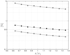
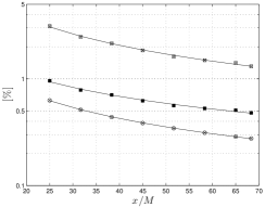
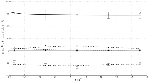
Figure 2: Homogeneity assessment for the fractal square grid in the decay region around the centerline for $U_{\infty}=15ms^{-1}$. Top figures: dimensionless streamwise inhomogeneity measures (▫❌) $\frac{L_{u}}{\overline{u^{2}}}\frac{\partial\overline{u^{2}}}{\partial x}$, (▪) $\frac{L_{u}}{\lambda}\frac{\partial\lambda}{\partial x}$, (○❌) $\frac{\partial L_{u}}{\partial x}$ for the (a) fractal square grid (SFG), (b) regular grid (RG). Bottom figure: (c) T.K.E budget (9) normalised by the dissipation for the SFG at the centreline, (▫) $\varepsilon_{LS}$ - advection, (○) $\mathcal{P}$ - production, (◃) $\mathcal{T}$ - triple-correlation transport, (●) $\Pi$ - pressure transport, ($\star$) $\mathcal{D}_{\nu}$ - viscous diffusion.

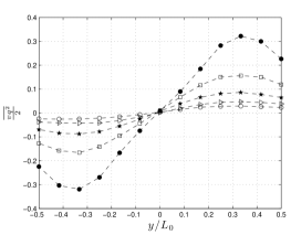
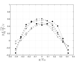
Figure 3: Transverse profiles of (a) $\frac{\overline{vq^{2}}}{2}$, (b) $2\frac{d}{dy}\frac{\overline{vq^{2}}}{2}/\varepsilon$ at five streamwise downstream positions and $U_{\infty}=15ms^{-1}$: (●) $x/x_{\star}=0.63$, (▫) $x/x_{\star}=0.83$, ($\star$) $x/x_{\star}=1.04$, (▹) $x/x_{\star}=1.24$, (○) $x/x_{\star}=1.44$

Table 4: Turbulence statistics for five streamwise locations recorded at $U_{\infty}=15ms^{-1}$.

Position(mm)	1850	2450	3050	3650	4250
$x/x_{*}$	0.63	0.83	1.04	1.24	1.44
$Re_{\lambda}$	352	292	253	226	210
$\sqrt{\overline{u^{2}}}$ [ms-1]	1.28	0.99	0.79	0.65	0.56
$L_{u}$ [mm]	45.7	47.6	50.0	50.7	53.6
$\lambda$ [mm]	4.1	4.4	4.8	5.2	5.6
$\eta$ [mm]	0.11	0.13	0.15	0.18	0.2
$\varepsilon_{LS}\equiv-\frac{U}{2}\frac{\partial}{\partial x}\overline{u^{2}}\left(1+2\frac{\overline{v^{2}}}{\overline{u^{2}}}\right)$ [m2s-3]	28.6	13.9	7.7	4.7	3.0
$\varepsilon_{iso}^{SW}\equiv 15\nu\overline{\left(\frac{\partial u}{\partial x}\right)^{2}}$ [m2s-3]	21.6	11.1	6.0	3.5	2.2
$\varepsilon_{iso}^{XW}\equiv 3\nu\overline{\left(\frac{\partial u}{\partial x}\right)^{2}}+6\nu\overline{\left(\frac{\partial v}{\partial x}\right)^{2}}$ [m2s-3]	16.6	8.7	4.7	3.1	1.7
-$\overline{u^{2}}\frac{\partial U}{\partial x}$ [m2s-3]	0.62	0.27	0.11	0.07	0.05
$-2\overline{uv}\frac{\partial U}{\partial y}$ [m2s-3]	1.32	0.12	0.04	0.004	0.0007
$\frac{\partial}{\partial x}\frac{\overline{uq^{2}}}{2}$ [m2s-3]	0.69	0.39	0.06	-0.01	-0.004
$2\frac{\partial}{\partial y}\frac{\overline{vq^{2}}}{2}$ [m2s-3]	8.22	5.53	3.25	1.83	1.08
$\nu\frac{\partial^{2}\overline{q^{2}}}{\partial x^{2}}$$(\times 10^{5})$ [m2s-3]	4.23	1.72	0.81	0.42	0.024
$-\nu\frac{\partial^{2}\overline{q^{2}}}{\partial y^{2}}$$(\times 10^{3})$ [m2s-3]	3.24	1.55	1.29	1.08	0.45
$\sqrt{\overline{u^{2}}/\overline{v^{2}}}$	1.15	1.13	1.11	1.13	1.10
$\frac{\overline{(dv/dx)^{2}}}{\overline{(du/dx)^{2}}}$	1.39	1.40	1.42	1.44	1.46
$L_{u}/L_{v}$	3.7	3.2	3.0	2.7	3.0

3.2.2 Isotropy

The simplest assessment of large-scale anisotropy is achieved by comparing the ratio of streamwise and transverse r.m.s. velocity components, sometimes referred to as isotropy factor. The results of such measurements at the centreline are presented in table 4 and show a fair agreement with Hurst & Vassilicos (2007) for the same set-up, confirming that the flow is reasonably isotropic for all the assessed decay region, $u^{\prime}/v^{\prime}\approx 1.1-1.25$. The range of isotropy factors encountered in our flow are comparable to those obtained by Mydlarski & Warhaft (1996) for their active grids, although further research shows it is possible to tune the active grid to decrease the anisotropy of the flow (Kang, Chester & Meneveau, 2003). Similarly it should be possible to further optimise the design of the fractal grids to increase isotropy, e.g. by increasing the thickness ratio as is suggested by the data presented by Hurst & Vassilicos (2007). Hurst & Vassilicos (2007) also reported the ratio between the longitudinal and transversal integral length-scales ($L_{u}$ and $L_{v}$) for the same low-blockage space-filling fractal square grid to be $L_{u}/L_{v}\approx 2$, but this is not confirmed by the present data where the integral scales ratio is larger than 2 as shown in table 4, even though this ratio decreases further downstream. This discrepancy is likely due to the calculation method of the transversal integral scales; integrating the transverse correlation function to the first zero crossing as Hurst & Vassilicos (2007) (incorrectly) did we recover an integral scale ratio closer to 2.

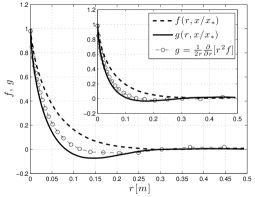
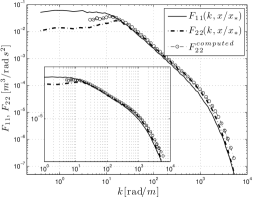
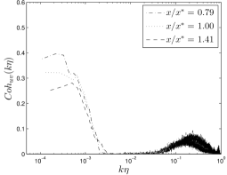
Figure 4: Longitudinal and transversal one-dimensional (a) correlation function (b) energy spectra for $x/x_{*}=0.63$ (and for $x/x_{*}=1.4$ in the insert); (c) coherence spectra in the coordinate system rotated $45^{\circ}$ with respect to the flow direction. $U_{\infty}=15ms^{-1}$.

A complementary assessment of isotropy is obtained by computing the longitudinal and transversal correlation functions, $f(r,x)\equiv\overline{u(x)u(x+r)}/\overline{u(x)^{2}}$ and $g(r,x)\equiv\overline{v(x)v(x+r)}/\overline{v(x)^{2}}$ , and comparing $g(r,x)$ with $g^{iso}(r)=\frac{1}{2r}d[r^{2}f(r)]/dr$ which is the relation between the two correlation functions in the presence of isotropy. The comparison is shown in figure 4a for two downstream locations and it can be seen that there is a modest agreement between the measured and computed transverse correlation functions, although the agreement improves downstream. A similar comparison in spectral space is shown in figure 4b, where the isotropic relation between the longitudinal and transversal one-dimensional spectra is: $F_{22}^{iso}=\left[F_{11}+k_{1}dF_{11}/dk_{1}\right]/2$. There is a fair agreement between the measured and computed transverse one-dimensional spectra in the ’inertial region’, but not at the low wave-numbers (which is consistent with $L_{u}/L_{v}>2$) nor at high wave-numbers (reflecting that $\overline{(dv/dx)^{2}}/\overline{(du/dx)^{2}}<2$). This lack of small-scale isotropy was not reported by Seoud & Vassilicos (2007) nor by Mydlarski & Warhaft (1996) in their active-grid experiments because they filtered out the highest frequencies where their cross wire measurements could not be trusted. Note that in agreement with the latter experiments the coherence spectra (figure 4c) show that the anisotropy (inferred by the cross-correlation of the velocity components in a coordinate system rotated by $45^{\circ}$) is mostly contained in the large scales. The cause for this, perhaps apparent, small-scale anisotropy in figure 4 and in our values of $\overline{(dv/dx)^{2}}/\overline{(du/dx)^{2}}$ in table 4 is most probably the separation between the cross-wires ($\approx 1mm$) being up to ten times the Kolmogorov length-scale. It should be noted that, precisely because of this problem, the velocity derivative ratios in Seoud & Vassilicos (2007) were obtained for a low-pass filtered velocity signal at $k\eta\approx 0.1$. This way, these authors obtained $\overline{(dv/dx)^{2}}/\overline{(du/dx)^{2}}\simeq 2$ even though strictly speaking $\overline{(du_{i}/dx)^{2}}=\int_{0}^{\infty}\!k_{1}^{2}F_{ii}(k_{1})\,dk_{1}$, where contributions coming from $k\eta>10^{-1}$ cannot necessarily be written off as negligible.

3.2.3 Wind-tunnel confinement

A qualitative assessment of the effect of flow confinement in wind-tunnel experiments can be made by comparing the tunnel’s height/width with the flow’s integral scale and comparing the ratio with similar experiments and with DNS. For simplicity we take the longitudinal integral scale at the centreline to be the representative scale for each transverse section and it is typically 8.5 to 10 times smaller than the wind-tunnel width. This is just about in-line with what is typically used in DNS of decaying homogeneous turbulence Ishida, Davidson & Kaneda (2006); Wang & George (2002), considering the boundary-layers on the wind-tunnels walls which reduce the effective transverse size of the tunnel down to 8 times the integral scale (based on the displacement thickness of the boundary-layers) very far downstream. The active-grid experiments by Mydlarski & Warhaft (1996) were performed at equivalent $Re_{\lambda}$ in a similar sized wind-tunnel and produced larger integral-scales but were in line with typical decay properties and did not observe any of the outstanding features of our flow reported in the Subsections 3.3, 3.4 and 3.5 below. It is therefore unlikely that our results, namely the abnormally high decay exponent and the proportionality between the integral and the Taylor micro-scale, may be due to confinement. However it is conceivable that the effective choking of the tunnel by the growing boundary layers very far downstream does have some effect on the larger turbulence scales at these very far distances (see figure 5).

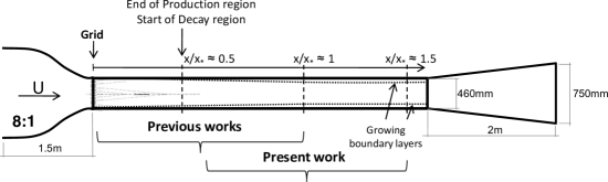
Figure 5: Sketch of the wind-tunnel where the decay of turbulence generated by regular and fractal square grids was measured. This wind-tunnel is a modified version, with an extended test section, of the wind-tunnel used by Hurst & Vassilicos (2007), Seoud & Vassilicos (2007) and Mazellier & Vassilicos (2010) in their experimental investigations of fractal generated turbulence. The boundary layers developing at the wall were estimated to have a displacement thickness of $\delta_{1}\approx 4mm$ at $x=2m$ ($x/x_{*}=0.7$), $\delta_{1}\approx 8mm$ at $x=3.5m$ ($x/x_{*}=1.2$) and $\delta_{1}\approx 10mm$ at $x=4.5m$ ($x/x_{*}=1.5$).

3.3 Normalised energy dissipation rate

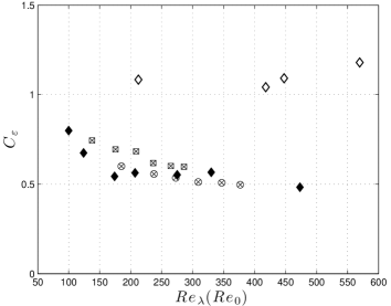
Figure 6: Normalised energy dissipation rate $C_{\varepsilon}$ versus $Re_{\lambda}$ with $Re_{\lambda}$ changing as a function of the inlet Reynolds number $Re_{0}$ for a fixed streamwise downstream location for fractal square grid-, active grid- and regular grid-generated turbulence. For the fractal square grid data the inlet Reynolds number is changed by varying the free-stream speed between $5ms^{-1}<U_{\infty}<17.5ms^{-1}$ and is measured with a $l_{w}=0.45mm$ sensing length single-wire at two streamwise downstream positions: (○❌) $x/x_{*}=0.63$ and (▫❌) $x/x_{*}=1.04$. (⬫) Active grid data is taken from table 1 of Gamard & George (2000) which is based on the experimental data by Mydlarski & Warhaft (1996) (Gamard & George (2000) computed the longitudinal and the transverse integral scales from the spectra, but their latter estimate yielded less scatter, hence we assume isotropy and use twice the transverse integral scale). (⬪) Regular grid data from the data compilation by Sreenivasan (1984), figure 1 (only data by Kistler & Vrebalovich (1966) is used since no other experiment with more than one data point had $Re_{\lambda}>100$).

It follows from this paper’s introduction that for fully-developed turbulence generated by at least some space-filling low blockage fractal square grids, the normalised energy dissipation rate $C_{\varepsilon}$ depends both on an initial conditions/global Reynolds number $Re_{0}$ (e.g. $Re_{0}\equiv U_{\infty}x_{*}/\nu$) and on a local Reynolds number ($Re_{\lambda}(x)$). This distinction between two different Reynolds number dependencies follows from equations (1.5) and (1.7) and does not need to be made in the context of the Richardson-Kolmogorov phenomenology where the functions $A$ and $B$ are identical and the exponents $\alpha$ and $\beta$ are both equal to $1/2$.

The present measurements of the normalised energy dissipation rate $C_{\varepsilon}$ for different $Re_{0}$ (by varying $U_{\infty}$) at two fixed streamwise downstream positions from the fractal grid (figure 6) suggest that $C_{\varepsilon}(Re_{0})$ is roughly constant beyond $Re_{\lambda}(Re_{0})\approx 200$ (figure 6). From (1.7), this observation implies that, at high enough values of $Re_{0}$, $\alpha=\beta$ and

$$C_{\varepsilon}=15A({x-x_{0}\over x_{*}})/B({x-x_{0}\over x_{*}})$$ (10)

irrespetive of $Re_{0}$. The facts that $A$ is a slow-varying whereas $B$ is fast varying function of ${x-x_{0}\over x_{*}}$ is reflected in the steep increase of $C_{\varepsilon}$ with $x$ (see figure 7a). This is fundamentally different from the cornerstone assumption that $C_{\varepsilon}$ is constant, an assumption which is approximately verified by the turbulence generated by our regular grid provided $Re_{0}$ is large enough (see figure 7a).

The high $Re_{0}$ behaviour of $C_{\varepsilon}(Re_{0})$ is very comparable to that found with regular and active-grids at similar Reynolds numbers (figure 6) and more generally with other boundary-free turbulent flows such as various wakes (see e.g. Burattini et al., 2005; Pearson et al., 2002) and DNS of forced stationary homogeneous turbulence (see data compilations by Sreenivasan, 1998; Burattini et al., 2005). However, the fundamental difference with the present fractal square grid-generated turbulence is that the $C_{\varepsilon}$ asymptote for high $Re_{0}$ is different for different streamwise downstream locations. This is high Reynolds number non-Richardson-Kolmogorov behaviour

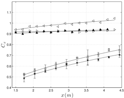
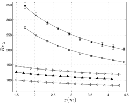
Figure 7: Normalised energy dissipation rate $C_{\varepsilon}$ and Reynolds number $Re_{\lambda}$ versus streamwise downstream location $x$ for both the square fractal grid (SFG) and regular grid (RG) data recorded at different inlet velocities: (▫) SFG at $U_{\infty}=10ms^{-1}$, ($\star$) SFG at $U_{\infty}=15ms^{-1}$, (◃) RG at $U_{\infty}=10ms^{-1}$, (▴) RG at $U_{\infty}=15ms^{-1}$, (▹) RG at $U_{\infty}=20ms^{-1}$. Since the square fractal grid data is acquired with three different wire resolutions (see Sec. 2.1) we plot the arithmetic mean plus error bars.

The key departure behind the present fractal square grid-generated turbulence behaviour lies in the difference between the streamwise dependencies of $L_{u}/\lambda$ and $Re_{\lambda}$ ($A(x)\neq B(x)$, see equations 1.4 and 1.5). For steady initial conditions (fixed $Re_{0}$) there is a significant $Re_{\lambda}$ decrease during decay (figure 7b), whereas $L_{u}/\lambda$ stays approximately constant (figure 8a), leading to a steep monotonic downstream increase in the normalised dissipation rate $C_{\varepsilon}$ (figure 7a) which follows approximately the form $C_{\varepsilon}\propto(L_{u}/\lambda)/Re_{\lambda}\sim Re_{\lambda}^{-1}$ (figure 8b). Note, in particular, how the $C_{\varepsilon}$ versus $Re_{\lambda}$ curve shifts to the right as $Re_{0}$ increases, which is clear evidence of the two independent dependencies that $C_{\varepsilon}$ has on $Re_{\lambda}$ and $Re_{0}$ in this fractal-generated turbulence.

Data were taken with probes of different spatial resolutions to confirm that these results are not meaningfully biased by the resolution of the measurements yielding figure 8 (see Sec. 2.1 for details). Nonetheless it can be seen that the lesser resolution probe ($d_{w}\approx 5\mu m$, $l_{w}\approx 1mm$) has a slightly lower $L_{u}/\lambda$ ratio due to the underestimation of $\overline{(\partial u/\partial x)^{2}}$, but it does not change the main observation that $L_{u}/\lambda$ is effectively roughly constant, at least compared to the wide variation of $Re_{\lambda}$, during decay.

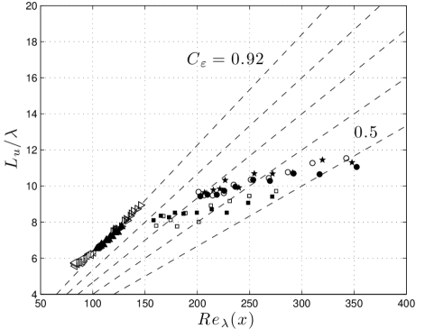
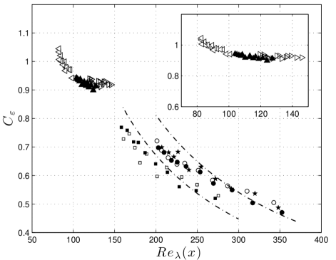
Figure 8: Local Reynolds number dependence $Re_{\lambda}(x)$ of (a) Integral length scale to Taylor micro-scale ratio $L_{u}/\lambda$ and (b) normalised energy dissipation rate $C_{\varepsilon}$, for both the square fractal grid (SFG) and regular grid (RG) data recorded at different inlet velocities with single-wire (SW): (▪) SFG recorded at $U_{\infty}=10ms^{-1}$ with a $l_{w}=1mm$ sensing length SW, (▫) SFG at $U_{\infty}=10ms^{-1}$, $l_{w}=0.45mm$, (●) SFG at $U_{\infty}=15ms^{-1}$, $l_{w}=1mm$, (○) SFG at $U_{\infty}=15ms^{-1}$, $l_{w}=0.45mm$, ($\star$) SFG at $U_{\infty}=15ms^{-1}$, $l_{w}=0.2mm$, (◃) RG at $U_{\infty}=10ms^{-1}$, $l_{w}=0.45mm$, (▴) RG at $U_{\infty}=15ms^{-1}$, $l_{w}=0.45mm$, (▹) RG at $U_{\infty}=20ms^{-1}$, $l_{w}=0.45mm$. The dashed-dot lines follow the form $\propto Re_{\lambda}^{-1}$. The insert of the second figure is a zoomed plot of the RG data.

We now contrast the behaviour of our fractal square grid-generated turbulence behaviour with that of turbulence generated by regular-grid. Such turbulence is thought to follow Richardson-Kolmogorov phenomenology, although it’s usually difficult to exceed Reynolds numbers beyond $Re_{\lambda}\approx 150$ in typically sized laboratory wind-tunnels (at least if Corrsin’s restriction $x/M>30$ is applied, Corrsin (1963)) and therefore the regular grid experiments are commonly at the lower end of the range of validity of the Richardson-Kolmogorov phenomenology. Nevertheless, our regular grid data for $U_{\infty}=20ms^{-1}$ appear to have sufficiently high Reynolds numbers to support $C_{\varepsilon}\approx const$ (figure 8b) and related $L_{u}/\lambda\propto Re_{\lambda}$ (figure 8a). Furthermore it can be seen that the $Re_{\lambda}$ dependence of $C_{\varepsilon}$ falls on the same curve regardless of how $Re_{\lambda}$ is varied, whether by varying $Re_{0}$ or by varying the streamwise position of the measurement. The same observation can be made for the curve $L_{u}/\lambda$ versus $Re_{\lambda}$. This is well-defined Richardson-Kolmogorov behaviour where $A(x)=B(x)$, $\alpha=\beta=1/2$ and consequently no distinction between local and global Reynolds number exists. Below $Re_{\lambda}\approx 120$ direct dissipation becomes noticeable and causes a departure from $C_{\varepsilon}\approx const$, presumably due to an insufficiently large separation between outer and inner scales Dimotakis (2000).

Summarising, the present fractal square grid-generated decaying turbulence is fundamentally and qualitatively different from regular grid-generated decaying turbulence. The $C_{\varepsilon}\approx const$ behaviour is not observed in figure 8 for the fractal square grid despite the moderately large turbulent Reynolds numbers $Re_{\lambda}$ (around three times the $Re_{\lambda}$ necessary for the regular grid to exhibit $C_{\varepsilon}=const$ on this plot) and the evidence that the global/inlet Reynolds number $Re_{0}$ is sufficiently large for $C_{\varepsilon}$ to be independent of $Re_{0}$ (figure 6). In fact the normalised dissipation rate is closer to $C_{\varepsilon}\sim Re_{\lambda}^{-1}$ and $L_{u}/\lambda\approx const$, which is in line with the previous experiments by Mazellier & Vassilicos (2010), although the larger length of the present wind-tunnel brings to evidence that $L_{u}/\lambda$ and $C_{\varepsilon}Re_{\lambda}$ are not exactly constant in this tunnel, but are only roughly so for all the assessed decay region. This might be an effect brought about, perhaps paradoxically, by the eventual low (though not too low) values of $Re_{\lambda}$ far downstream. Or it might be due to a decrease in the growth of $L_{u}$ because of the boundary layers at the tunnel walls which begin to have a significant thickness very far downstream in this longer wind-tunnel. As this wall effect might not affect the growth of $\lambda$, $L_{u}/\lambda$ would monotonically decrease downstream. Nevertheless, as we show further down in this paper, the downstream evolutions of $L_{u}/\lambda$ and $C_{\varepsilon}$ are consistent with a self-preserving evolution of energy spectra which can be made to collapse with a single-scale reasonably well, as opposed to the two different inner and outer scales required by Richardson-Kolmogorov phenomenology.

Finally note that the large and small scale anisotropy ( characterised by the ratios $u^{\prime}/v^{\prime}\approx 1.1$ and $\overline{(dv/dx)^{2}}/\overline{(du/dx)^{2}}\approx 1.5$, see Sec. 3.2.2 and table 4) change the exact numerical values of $C_{\varepsilon}$ and $Re_{\lambda}$ for each measurement location (see figure 9) and can be considered a source of uncertainty. Nevertheless, the main difference is an offset of the $C_{\varepsilon}$ versus $Re_{\lambda}$ curve and there is no meaningful change of its functional form.

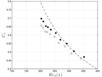
Figure 9: Uncertainty & bias due to large and small scale (an)isotropy in the observed normalised energy dissipation rate $C_{\varepsilon}$ behaviour. In this specific plot we re-define $u^{\prime 2}$ and $\varepsilon$ to be $u^{\prime 2}\equiv\overline{u^{2}}(1+2\overline{v^{2}}/\overline{u^{2}})$, $\varepsilon\equiv\nu\,\overline{(du/dx)^{2}}[3+6\overline{(dv/dx)^{2}}/\overline{(du/dx)^{2}}]$ and take(●) the isotropic estimates $\overline{v^{2}}/\overline{u^{2}}=1$ and $\overline{(dv/dx)^{2}}/\overline{(du/dx)^{2}}=2$ and (○) the anisotropy estimates of $\overline{v^{2}}/\overline{u^{2}}$ and $\overline{(dv/dx)^{2}}/\overline{(du/dx)^{2}}$ from table 4. The dashed-dot line follows $\propto Re_{\lambda}^{-1}$

3.4 Energy decay

The functional form of the turbulent kinetic energy decay is usually assumed to follow a power-law, which is mostly in agreement with the large database of laboratory and numerical experiments for both grid-generated turbulence and boundary-free turbulent flows

$$\overline{u^{2}}\sim(x-x_{0})^{-n}$$ (11)

where $\overline{u^{2}}\equiv u^{\prime 2}$.

Mazellier & Vassilicos (2010) proposed a convenient alternative functional form for the kinetic energy decay (and for the evolution of $\lambda$ when $U_{\infty}{d\over dx}\overline{u^{2}}\propto\nu\overline{u^{2}}/\lambda^{2}$ is a good approximation) that is both consistent with the power-law decay and the exponential decay law proposed by George & Wang (2009):

$$\left\{\begin{aligned} \lambda^{2}=\lambda_{0}^{2}&\left[1+\frac{4\nu a|c|}{l^{2}(x_{0})U_{\infty}}(x-x^{\prime}_{0})\right]\\ \overline{u^{2}}=\frac{2\,u^{\prime 2}_{0}}{3}&\left[1+\frac{4\nu a|c|}{l^{2}(x_{0})U_{\infty}}(x-x^{\prime}_{0})\right]^{(1-c)/2c}\end{aligned}\right.$$ (12)

where $c<0$. In the limit of $c\rightarrow 0$ it asymptotes to an exponential decay with constant length-scales throughout the decay, but otherwise it is a power-law decay where $x_{0}$ is not the conventional virtual origin where the kinetic energy is singular. The two equations (11) & (12) are equivalent with $n=(c-1)/2c$ and $x_{0}=x^{\prime}_{0}-l^{2}_{0}\,U_{\infty}/(4\nu ac)$.

Determining the decay exponent directly from (11) is difficult, although feasible, since a non-linear fit is generally needed to determine $n$ and $x^{\prime}_{0}$ simultaneously. For homogeneous (isotropic) turbulent decaying flow where advection balances dissipation it is possible to obtain a linear equation for the Taylor micro-scale that can be used to determine the virtual origin, thus simplifying the task of determining the decay exponent. Using $\lambda^{2}=15\nu\overline{u^{2}}/\varepsilon$ in conjunction with the advection dissipation balance characteristic of homogeneous isotropic turbulence ($3/2\,U\partial\overline{u^{2}}/\partial x=-\varepsilon$) and assuming power-law energy decay (11) we get

$$\lambda^{2}=\frac{10\,\nu}{n\,U}(x-x_{0}).$$ (13)

Note that for $\lambda^{2}$ to be linear the mean velocity has to be constant otherwise the linear relation holds for $U\lambda^{2}$. Even though advection does not balance dissipation in our fractal grid-generated decaying turbulence because of the significant presence of transverse energy transport as shown in Sec. 3.2.1, transverse energy transport and dissipation remain approximately proportional to each other throughout the assessed decay region and for the range of values of $U_{\infty}$ tried here. This suggests that

$$U{d\over dx}\overline{u^{2}}\propto\nu\overline{u^{2}}/\lambda^{2}$$ (14)

might be a good approximation for the decay region of our fractal-generated turbulence as is indeed supported by our data which show that U$\lambda^{2}$ grows linearly with downstream location and even that $U\lambda^{2}$ versus $x$ collapses the data well for different inlet velocities $U_{\infty}$ (see figure 10a).

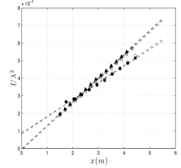
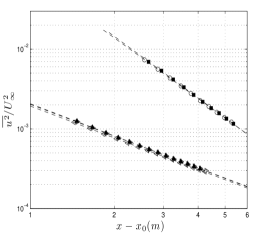
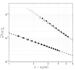
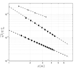
Figure 10: Decay of turbulence generated by the regular (RG) and the fractal square (SFG) grid: (a) linear growth of $U\lambda^{2}$ (b) power-law fit using method I, (c) power-law fit using method III (d) power-law fit using method IV. (▪) SFG at $U_{\infty}=10ms^{-1}$, (○) SFG at $U_{\infty}=15ms^{-1}$, (◃) RG at $U_{\infty}=10ms^{-1}$, (▴) RG at $U_{\infty}=15ms^{-1}$, (▹) RG at $U_{\infty}=20ms^{-1}$, ($\smallstar$) data from the Active-grid experiment by Mydlarski & Warhaft (1996).

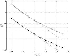
Figure 11: Turbulent kinetic energy decay of turbulence generated by the fractal square grid fitted to (12) using method II (dashed-dot line) and method III (solid line). The data range used in method II is $0.6<x/x_{*}<1.1$, which corresponds to the streamwise region assessed by Mazellier & Vassilicos (2010). Streamwise data was taken at two fixed inlet velocities: (▪) $U_{\infty}=10ms^{-1}$, (○) $U_{\infty}=15ms^{-1}$. Notice that for $0.6<x/x_{*}<1.1$ the two methods appear to fit the data reasonably well, but further downstream the differences become evident.

The decay exponents of (11) and (12) are estimated using four alternative methods:

• Method I: linear fit to $U\lambda^{2}$ (13) to determine the virtual origin followed by a linear fit to the logarithm of (11) to determine the exponent $n$, as done by Hurst & Vassilicos (2007). Antonia et al. (2003) determined the virtual origin in a similar fashion by plotting $\lambda^{2}/(x-x_{0})$ for different $x_{0}$ and choosing the virtual origin yielding the broadest plateau (which for their regular grid experiment was $x_{0}\approx 0$).

• Method II: the linearised logarithm method proposed in Mazellier & Vassilicos (2010) to determine the unknowns in (12).

• Method III: direct application of a non-linear least-squares regression algorithm (’NLINFIT’ routine in MATLAB^TM) to determine the decay exponent and virtual origin simultaneously. This is related to the method used by Lavoie, Djenidi & Antonia (2007), but allowing the virtual origin to be determined by the algorithm as well. This method can be applied to (11) as well as to (12). Note that if applied to (11) as we do here, this fitting method does not necessarily yield a virtual origin compatible with (13).

• Method IV: assume the virtual origin coincides with the grid location and linearly fit the logarithm of (11). This crude method typically yields biased estimates of the decay exponent, since there is no a priori reason for the virtual origin to be zero. Nevertheless this is a robust method typically used to get first order estimates of power law decay exponents in many flows (e.g. the active-grid data by Mydlarski & Warhaft, 1996).
  

Grid	U	Method I		Method II	Method III		Method IV
	$(ms^{-1})$	n	$x_{0}/x_{*}$	$(1+c)/2c$	n	$x_{0}/x_{*}$
RG	10	1.32	0.18	4.34	1.25	0.53	1.36
RG	15	1.34	0.08	5.04	1.25	0.52	1.36
RG	20	1.32	0.06	5.47	1.21	0.63	1.33
SFG	10	2.57	-0.31	7.10	2.51	-0.28	1.93
SFG	15	2.53	-0.28	8.01	2.41	-0.22	1.95

Table 5: Decay exponents and virtual origin estimation using different methods

A main difference between these methods is the way of determining the virtual origin, which has an important influence on the decay exponent extracted. This inherent difficulty in accurately determining the decay exponent is widely recognised in the literature (see e.g.  Mohamed & LaRue, 1990).

The decay data for the regular grid- and fractal square grid-generated turbulence are well approximated by the curve fits obtained from methods I & III (see figures 10b & 10c) and the numerical values of the exponents change only marginally (see table 5). On the other hand method IV also seems to fit the data reasonably well (see figures 10d) but the exponents retrieved for the fractal grid data are $n\approx 2$, slightly lower than the exponents predicted by the other methods $n\approx 2.5$. The virtual origin which is forced to $x_{0}=0$ in method IV leads to a slight curvature in the $\log(\overline{u^{2}})$ versus $\log(x)$ data (almost imperceptible to the eye, compare the fractal grid data in figures 10c & 10d) and a non-negligible bias in the estimated exponents. Nevertheless the difference in the power laws describing the measured regular grid- and square fractal grid-generated turbulence is quite clear. For completeness, the results from the experimental investigation by Mydlarski & Warhaft (1996) on decaying active grid-generated turbulence are added in figure 10d. They applied a fitting method equivalent to method IV and reported a power-law fit yielding a decay exponent $n=1.21$. Kang et al. (2003) employed the same method to their active grid-generated turbulence data and retrieved a similar result, $n=1.25$.

Note that there are residual longitudinal mean velocity gradients (which cause a residual turbulence production of about $3\%$ of the dissipation, see Sec 3.2.1) and therefore it is preferred to fit $\overline{u^{2}}$ data rather than $\overline{u^{2}}/U^{2}$ data. Nevertheless we checked that fitting $\overline{u^{2}}/U^{2}$ data does not meaningfully change the results nor the conclusions.

Concerning method II it can be seen (table 5) to be the most discrepant of the four methods yielding a much larger decay exponent. This method was proposed by Mazellier & Vassilicos (2010) to fit the general decay law (12) and is based on the linearisation of the logarithm appearing in the logarithmic form of (12), i.e.

$$\log(u^{\prime 2})=\log\left(\frac{2\,u^{\prime 2}_{0}}{3}\right)+\left[-\frac{1+c}{2c}\right]\log\left(1+\frac{4\nu ac}{\lambda_{0}^{2}U_{\infty}}(x-x^{\prime}_{0})\right).$$ (15)

Linearisation of the second logarithm on the right hand side of (15) assumes $\frac{4\nu ac}{\lambda_{0}^{2}U_{\infty}}(x-x^{\prime}_{0})<<1$. This quantity, as we have confirmed in our data, is indeed smaller than unity and for the farthest position $4\nu ac/(l^{2}(x_{0})U_{\infty})(x-x_{0})\approx 0.3$, but the fact that this linearised method does not yield results comparable to methods I and III suggests that the linearisation of the logarithm may be an oversimplification. In figure 11 the kinetic energy decay data of turbulence generated by the fractal square grid is shown along with the fitted curves obtained from methods II and III in a plot with a logarithmic ordinate and a linear abscissa. In figure 11a the data taken at positions beyond $x/x_{*}\approx 1.05$ are excluded in order to compare with the results presented in Mazellier & Vassilicos (2010) where the data range was limited to $0.5<x/x_{*}<1.05$. Visually, in figure 11a, the two different fitting methods appear to fit the data reasonably well and thus the linearisation of the logarithm in (15) is justified in this limited range. Note, however, that the two fitting methods yield very different decay exponents because they also effectively yield different virtual origins: for example at $U_{\infty}=15ms^{-1}$ method III yields $(1+c)/(2c)\approx-2.4$ whereas method II yields $(1+c)/(2c)\approx-8.0$. In figure 11b, where no data is excluded, it can clearly be seen that the two methods produce very different curves and very different decay exponents (note however that the use of a longer test section, which allows the assessment of the decay behaviour further downstream, comes at the cost of having thicker boundary layers developing at the walls which can have an increasing influence on the largest turbulent eddies, as discussed in Sec. 3.2.3).

3.4.1 Influence of transverse transport on power-law decay exponent

It is shown in Sec. 3.2.1 that dissipation does not balance the advection but that the two are roughly proportional throughout the measured decay region of the fractal square grid-generated turbulence. It is also shown in that section that this imbalance is mostly due to transverse triple-correlation transport which remains roughly $50-60\%$ of the dissipation throughout the measured region (with no clear increasing or decreasing trend), whereas turbulence production and longitudinal triple-correlation transport terms become negligible well before $x<x_{*}$. Pressure transport, calculated from the kinetic energy balance, may also play a noticeable role of countering a fraction (typically between $1/4$ and $1/3$) of the triple-correlation transport. Based on these results, equation (9) which holds at the centreline reduces to

$$\frac{U}{2}\frac{\partial\,\overline{q^{2}}}{\partial x}=-\varepsilon+\left[-2\frac{\partial}{\partial y}\frac{\overline{vq^{2}}}{2}+\Pi\right].$$ (16)

The decay rate of the kinetic energy as the turbulence is advected downstream (effectively the advection term) is now determined both by viscous dissipation and by a net effect of removing energy from the centreline and transporting it to the sides. As in the portion of the decay region of the fractal-generated turbulence where we take measurements this loss rate to the sides remains approximately proportional to the dissipation rate, i.e.

$$\frac{U}{2}\frac{\partial\,\overline{q^{2}}}{\partial x}=-\chi\,\varepsilon$$

where $\chi=1+[\,\partial\overline{vq^{2}}\partial y-\Pi\,]/\varepsilon\approx 1.5$ (figure 2c), we can expect the decay exponent $n$ to be set by the dissipation rate $\varepsilon$ (irrespective of what sets the dissipation rate). Indeed, the higher power law decay exponents exhibited by the fractal-generated turbulence can be accounted for by the fact that $C_{\varepsilon}\sim Re_{\lambda}^{-1}$ (see Sec. 3.3) and consequently the steep increase of $C_{\varepsilon}=\varepsilon L_{u}/u^{\prime 3}$ with streamwise location. In other words, an increasing proportion of $u^{\prime 3}/L_{u}$ is being dissipated at increasing streamwise locations which leads to an increase in the power law decay exponent relative to the $C_{\varepsilon}=const$ case.

In figure 12 we plot in logarithmic axes the streamwise decay of the advection, the dissipation and the transverse triple-correlation transport (which are all measured independently) and they indeed seem to follow straight lines (i.e. power laws) with the same slope (i.e. power law exponent), thus supporting our argument.

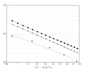
Figure 12: Downstream decay of: (●) kinetic energy $\frac{U}{2}\frac{\partial\overline{q^{2}}}{\partial x}$, (▫) dissipation $\varepsilon$, ($\star$) transverse triple-correlation transport $2\frac{\partial}{\partial y}\left(\frac{\overline{vq^{2}}}{2}\right)$, for $U=15ms^{-1}$

To further substantiate our argumentation one more set of experiments were conducted. Anemometry measurements at an inlet velocity of $U_{\infty}=15ms^{-1}$ using a $l_{w}=0.5mm$ sensing length single-wire were recorded between $0.63<x/x_{*}<1.44$ along four parallel lines aligned with the mean flow and crossing the grid at $z=0,\,0,\,20,\,20\,mm$ and $y=0,\,40,\,80,\,120\,mm$ ($z=0$ is the vertical plane of symmetry of the grid). From the transverse triple-correlation transport measurements for $z=0$ (figure 3b) we expect the contribution from this term to be very different at the centreline (where it is maximal) and off the centreline where is can be roughly zero ($y\approx 80$) or negative ($y>100$). However, if a value of $\chi$ can be defined that is constant throughout the streamwise decay range assessed here for each transverse $(y,z)$ position, then the argument outlined in the previous two paragraphs will hold even if $\chi$ varies with transverse positions, as indeed it does. The consequence is that, in the decay region assessed, the decay exponent n should remain about the same at all these transverse positions and also remain unusually large due to the $C_{\varepsilon}$ behaviour. The data for the different transverse locations are fitted using method III and the results (see table 6) are encouraging. In spite of some variation in the best fit power-law decay exponents, the numerical values of these exponents are all relatively close to each other ranging between $2.3$ and $2.6$. We note that these exponents are larger than all boundary-free turbulent flows listed in table 1.

Finally, as some presence of turbulence production and longitudinal transport remains for some distance downstream of $x_{peak}\approx 0.45x_{*}$ (though not in any significant way beyond $x_{*}$) we explore how the power-law fits of the turbulence energy decay change when the smallest streamwise location considered in the fit is increased. We do this both for centreline and off-centreline data and report our results in figure 13. On the centreline the decay exponent and virtual origin remain approximately the same within the scatter ($n\approx 2.4,\,x_{0}/x_{*}\approx-0.3$), but they show a respectively decreasing/increasing tendency off-centreline up to $x/x_{*}\approx 0.8$. At any rate, the decay exponents $n>2.0$ for all our data.

Table 6: Decay law estimates along four parallel streamwise oriented lines at the centreline and off the centreline between $0.63<x/x_{\star}<1.40$ obtained from method III.

y (mm)	n	$x_{0}/x_{\star}$
0	2.42	-0.27
40	2.61	-0.29
80	2.27	-0.11
120	2.63	-0.39

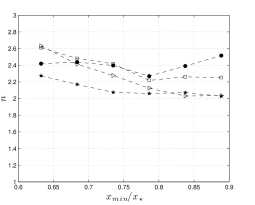
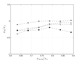
Figure 13: Decay law estimates for different data ranges $x_{min}<x/x_{\star}<1.40$, $U=15ms^{-1}$: (●) $y=0mm$, (▫) $y=40mm$, ($\star$) $y=80mm$, (▹) $y=120mm$. (a) decay exponent $n$ and (b) virtual origin $x_{0}/x_{\star}$ obtained from method III

In conclusion the decay exponents for the present fractal-generated turbulence measured both at the centreline and off the centreline in the region $0.6<x/x_{*}<1.5$ are consistently higher than those in all boundary-free turbulent flows listed in table 1 and much higher (by a factor between 4/3 and 2) than those of decaying turbulence generated by regular and active grids Mydlarski & Warhaft (1996); Kang et al. (2003). It might be interesting to note that in many boundary-free turbulent flows a conserved quantity such as $u^{\prime 2}L^{M+1}=const$ exists. Look at table 1 and note that $M=1,\,3,\,5,\,7$ for the four wakes, $M=-1$ for the mixing layer, $M=0,\,1$ for the jets and $M\geq 2$ for regular-grid turbulence. If the flow is also such that $Udu^{\prime 2}/dx\propto-\varepsilon$ then $C_{\varepsilon}=const$ implies

$$n=\frac{2(M+1)}{M+3}$$

and $C_{\varepsilon}\sim Re_{\lambda}^{-1}$ implies

$$n=\frac{M+1}{2}$$

(which is larger than $n=2(M+1)/(M+3)$ provided that $M>1$). Considering, for example, the range $M\geq 2$, the exponent $n$ corresponding to $C_{\varepsilon}\sim Re_{\lambda}^{-1}$ is at least $5/4$ times larger than the exponent $n$ corresponding to $C_{\varepsilon}=const$, and is generally much larger. If $M=3$ or $M=4$ then $C_{\varepsilon}\sim Re_{\lambda}^{-1}$ implies $n=2$ or $n=2.5$, close to what is observed here, whereas $C_{\varepsilon}\sim const$ implies $n=4/3$ or $n=10/7$.

At this stage we do not have any proof that a conserved quantity such as $u^{\prime 2}L^{M+1}=const$ exists for our fractal-generated turbulence. The previous paragraph is therefore only indicative and serves to illustrate how a $C_{\varepsilon}$ which is a decreasing function of $Re_{\lambda}$ can cause the decay exponent to be significantly larger than a $C_{\varepsilon}$ which is constant during decay and can even return decay exponents comparable to the ones observed here. Of course the decaying turbulence we study in this work is not perfectly homogeneous and isotropic because of the presence of transverse turbulent transport of turbulent kinetic energy and therefore significant gradients of third-order one-point velocity correlations. As a consequence, a conserved quantity such as $u^{\prime 2}L^{M+1}=const$, if it exists, cannot result from a two-point equation such as the von-Kármán-Howarth equation for homogeneous turbulence (see Vassilicos, 2011). We leave the investigation of conserved quantities in third-order inhomogeneous decaying turbulence such as the present one for the future (we include gradients of pressure-velocity correlations in the term ”third-order inhomogeneous”).

Nevertheless, it is clear that the dissipation rate of kinetic energy is increasingly larger than $u^{\prime 3}/L$ as the turbulence moves further downstream in cases such as the present one where $C_{\varepsilon}$ increases in approximate proportion to $1/Re_{\lambda}$ as the turbulence and $Re_{\lambda}$ decay. In the absence of any other type of loss or gain of kinetic energy, and assuming no counter-effect of $C_{\varepsilon}$ on the integral scale, a much steeper decay (e.g. much larger exponent $n$) will result than if $C_{\varepsilon}$ was constant during decay. In the present case where loss of energy also occurs by turbulent transport, see equation (16), this conclusion can remain the same in the region assessed only if, in that region, the loss of energy by turbulent transport remains proportional to the loss of energy by dissipation, as indeed observed.

The question then naturally arises whether this balance between turbulent transport and dissipation persists for the entire decay range all the way to very large values of $x/x_{*}$, much larger than those accessible here. If it does, then the implication is that perfectly homogeneous isotropic turbulence is impossible at any stage of the decay. If it does not and if turbulent transport starts to decay much faster than dissipation beyond a certain $x/x_{*}$, then a turbulence that is third-order homogeneous and isotropic may well appear if it has the time to do so before the final stages of decay. If $C_{\varepsilon}$ continues to increase nearly as $1/Re_{\lambda}$ in such a third-order homogeneous isotropic turbulence then the decay will remain exceptionally fast with values of $n$ such as the present ones. However, it may be that the unusual behaviour observed here for the dissipation rate $\varepsilon$ (a two-point statistic) is in fact the result of gradients in particular one-point statistics such as third-order velocity correlations and pressure-velocity correlations, i.e. inhomogeneities. Either way, the consequences can be far reaching and call for much future research, in particular re-examinations of Reynolds number dependencies of $C_{\varepsilon}$ in all manner of turbulent flows, in particular boundary-free turbulent flows such as those listed in table 1.

As a final remark, note that the data points for transverse turbulent transport in figure 12 seem to curve downwards at high $x/x_{*}$. However we cannot extrapolate much from this observation as we do not measure pressure directly and we do not know how gradients of pressure-velocity correlations curve at high $x/x_{*}$.

3.5 Collapse of the energy spectra and structure functions

As explained in Seoud & Vassilicos (2007) and Mazellier & Vassilicos (2010) single-length-scale self-preserving energy spectra can allow for $L_{u}/\lambda=const$ during decay. This can be assessed by plotting the normalised energy spectra for different positions along the mean flow direction and evaluating the collapse of the data or the lack thereof. It should be mentioned that the three-dimensional energy spectrum and one-dimensional energy spectra can be shown to be equivalent for an isotropic flow. It should also be noted that the flow is not exactly isotropic as discussed in Sect. 3.2.2, so we might expect some effect on the spectral collapse.

3.5.1 One-dimensional energy spectra

We begin by illustrating the qualitative difference between the collapse of the normalised energy spectra (using large scale variables: $u^{\prime 2}$, $L_{u}$) of turbulence generated by the regular grid and by the fractal square grid, see figure 14. The data for the regular grid are taken in a region where $L_{u}/\lambda\propto Re_{\lambda}$ and $C_{\varepsilon}\approx const$, see figure 8. The normalised spectra measured in the lee of the regular grid show a good collapse at the low frequencies but not at the high frequencies, which is in-line with Kolmogorov’s theory. On the other hand it can be seen that the normalised turbulence spectra generated by the fractal square grid appears to collapse at all frequencies, in-line with the single-length-scale assumption as previously observed by Mazellier & Vassilicos (2010).

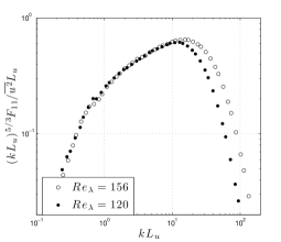
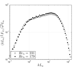
Figure 14: Compensated 1D energy spectra, normalised with $\overline{u^{2}},\,L_{u}$ at two streamwise locations for the (a) regular grid- and (b) fractal square grid-generated turbulence data. Both plots have roughly the same Reynolds number ratio, $Re_{\lambda_{1}}/Re_{\lambda_{2}}\approx 1.3$ (see Appendix A). The data are recorded at $U_{\infty}=20ms^{-1}$ and $U_{\infty}=10ms^{-1}$ respectively.

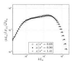
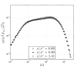
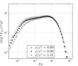
Figure 15: Compensated 1D energy spectra of turbulence generated by the fractal square grid at three streamwise downstream locations ($Re_{\lambda}=324,\,273,\,210$) at $U_{\infty}=15ms^{-1}$, normalised by (a) $\overline{u^{2}}$ and $L_{u}$ (b) $\overline{u^{2}}$ and $\lambda$ (c) $\nu$ and $\varepsilon$.

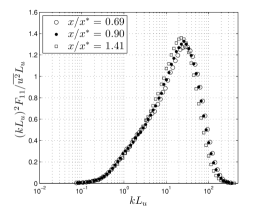
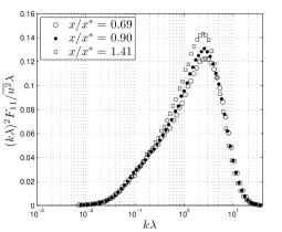
Figure 16: Compensated 1D energy spectra of turbulence generated by the fractal square grid at three streamwise downstream locations corresponding to $Re_{\lambda}=324,\,273,\,210$ at $U_{\infty}=15ms^{-1}$, normalised by (a) $\overline{u^{2}}$ and $L_{u}$ (b) $\overline{u^{2}}$ and $\lambda$.

In order to complement the previous results, the assessed decay region is extended allowing to further test the single-length-scale assumption. The normalised spectra of decaying turbulence downstream of our fractal square grid are shown in figure 15 using both the integral-scale and the Taylor micro-scale. For the extended region it can be seen that the normalised spectra using the Taylor micro-scale do collapse for the entire frequency range, although the collapse using the integral-scale at high frequencies is modest for $kL_{u}>40$ where the furthermost point ($x/x_{*}=1.41$) is taken into account. However the discrepancy between data at $Re_{\lambda}=324$ and $Re_{\lambda}=210$ is much too small compared to the lack of collapse which would occur if the data obeyed Richardson-Kolmogorov scaling as in figure 14a. It should be noted that in theory the collapses with $L_{u}$ or with $\lambda$ should be identical if $L_{u}\propto\lambda$, but as was seen in figure 8 this is not verified exactly in our wind-tunnel’s extended test section.

Nevertheless, in Appendix A we propose a methodology for making a rough estimate of the quality of collapse of normalised spectra at high frequencies and we find that it depends on the logarithm of the Reynolds number ratio $Re_{\lambda_{1}}/Re_{\lambda_{2}}$ at two streamwise distances $x=\xi_{1}$ and $x=\xi_{2}$ with a pre-factor which depends on the behaviour of $L_{u}/\lambda$ during decay. In the Appendix, we apply this methodology to the active grid data of Kang et al. (2003), for which there is evidence of a Richardson-Kolmogorov cascade, and show how spectral collapse with outer variables can be misleading because the Reynolds number ratio is small. The same methodology applied to our data shows that we are not fully able to conclude on the very high frequency end of fractal grid-generated energy spectra.

Pre-multiplying the 1D energy spectra by the square of the frequency yields the Fourier spectrum of $\overline{(du/dx)^{2}}$, so a second test to the single-length-scale assumption is to assess the collapse of this isotropic equivalent of the dissipation spectra. The data, plotted in figure 16 show a reasonable collapse onto a single curve using both length-scales, though it can be seen that the peak of the pre-multiplied spectra does not collapse perfectly. This may, to some extent, be an effect of the slight anisotropy of the flow, since it affects the large scale variables the normalisation is based on. It is shown in the following section how it is possible to partly account for this effect by computing the three-dimensional energy spectrum.

3.5.2 Three-dimensional energy spectra

The 3D energy spectrum is computed using the two-component velocity signal from the cross-wire measurements, with a similar algorithm to the one presented in Helland & Van Atta (1977). The central assumption of the algorithm is isotropy in order to relate the one-dimensional total energy spectrum $F_{ii}(k_{1})=F_{11}(k_{1})+F_{22}(k_{1})+F_{33}(k_{1})$ with the three-dimensional spectrum $E(k)$,

$$E(k)=-k_{1}\frac{dF_{ii}}{dk_{1}}$$ (17)

where the transverse one-dimensional spectra are considered to be approximately the same, i.e. $F_{22}(k_{1})\approx F_{33}(k_{1})$. The first derivative of the spectrum is computed using the logarithmic derivative proposed by Uberoi (1963):

$$E(k)=-F_{ii}\frac{d\ln F_{ii}}{d\ln k_{1}}$$

The 3D energy spectrum was evaluated at 50 logarithmically spaced frequencies, and a $2^{nd}$-order polynomial was fitted between two neighbouring frequencies using a least-squares-fit in order to obtain a smooth derivative of the spectrum.

From the 3D energy spectrum the integral scale $L$, the turbulent kinetic energy and the Taylor micro-scale can be recovered. The difficulty in accurately determining the low frequency range of the energy spectra and consequently estimating the integral length scale should be noted. For this reason, the assessment of the spectrum’s slope near $k\rightarrow 0$ was not possible.

The normalised compensated spectra are shown in figure 17, while the normalised enstrophy spectra are shown in figure 18. It is rewarding to see that the collapse of the 3D energy spectrum presents less scatter than the 1D spectrum thus offering support to the self-preserving single-length behaviour of turbulence generated by the fractal square grid. Hence, some of the deviation from single-scale self-similarity collapse of the 1D spectra in figures 15 & 16 is due to the moderate level of anisotropy present in the turbulence.

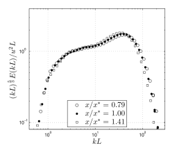
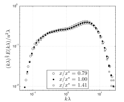
Figure 17: 3D energy spectra of turbulence generated by the fractal square grid at three streamwise downstream locations corresponding to $Re_{\lambda}=300,\,238,\,210$ at $U_{\infty}=15ms^{-1}$ and normalised by (a) $\overline{u^{2}}=2/3\overline{q^{2}}$ and $L$ (b) $\overline{u^{2}}$ and $\lambda$.

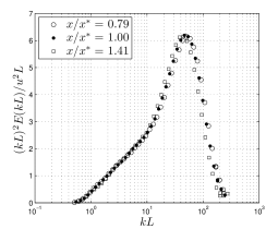
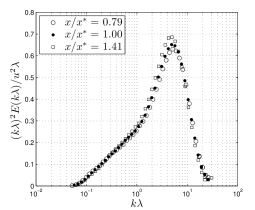
Figure 18: Enstrophy spectra of turbulence generated by the fractal square grid at three streamwise downstream locations corresponding to $Re_{\lambda}=300,\,238,\,210$ at $U_{\infty}=15ms^{-1}$ and normalised by (a) $\overline{u^{2}}=2/3\overline{q^{2}}$ and $L$ (b) $\overline{u^{2}}$ and $\lambda$.

3.5.3 Second-order structure functions

The collapse of the second order structure functions using $u^{\prime 2}$ and $L_{u}$ is shown in figure 19a. Similarly to what has already been discussed for the spectra, this structure function collapses well at both low and high separations in the case of our fractal-generated turbulence. However, this is clearly not the case for the turbulence generated by the regular grid (see figure 19b).

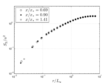
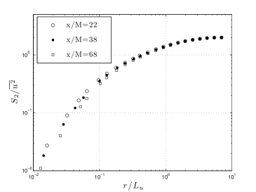
Figure 19: Second-order structure function at three streamwise downstream locations normalised by $\overline{u^{2}}$ and $L_{u}$: (a) SFG recorded at $U_{\infty}=15ms^{-1}$, $Re_{\lambda}=323,\,273,\,210$ for $x/x_{*}=0.69,0.90,1.41$ (b) RG recorded at $U_{\infty}=20ms^{-1}$, $Re_{\lambda}=156,\,137,\,120$ for $x/M=22,38,68$.

4 Conclusions and issues raised

The decay of regular grid- and fractal square grid-generated turbulence have been experimentally investigated using constant temperature hot-wire anemometry. The main contribution of the present work is to complement previous research on the decay of fractal grid-generated turbulence (e.g.  Hurst & Vassilicos, 2007; Seoud & Vassilicos, 2007; Mazellier & Vassilicos, 2010) by doubling the extent of the assessed decay region with the aim of investigating the persistence (or lack thereof) of the reported high decay exponents and the suppressed Richardson-Kolmogorov cascade. The present experimental investigation also complements the previous research by studying the effect of the hot-wire spatial resolution, carefully assessing the homogeneity of the flow during decay and taking anisotropy into account in the energy spectra.

We find that for streamwise downstream positions beyond $x/x_{*}\approx 0.6$ the turbulence is close to homogeneous except for a persistence of pressure transport and transverse energy transport and decays such that $L_{u}/\lambda\approx Const$ whilst $Re_{\lambda}$ sharply decreases, at least up to the furthermost downstream position investigated. However $L_{u}/\lambda$ increases with increasing grid Reynolds number, e.g. $Re_{0}=U_{\infty}t_{0}/\nu$. This observation is in direct conflict with the Richardson-Kolmogorov cascade Mazellier & Vassilicos (2010), believed to be dominant at this range of Taylor-based Reynolds numbers $Re_{\lambda}$ in various boundary-free turbulent flows, including regular grid- and active grid-generated turbulence Burattini et al. (2005); Sreenivasan (1984, 1998). It must be noted, however, that the vast majority of existing data is taken at fixed streamwise locations $x$ and varying inlet Reynolds numbers $Re_{0}$ and as we show in section 3.3 for fractal grid-generated turbulence, the streamwise downstream Reynolds number dependence $Re_{\lambda}(x)$ isn’t necessarily the same.

We observe that the energy spectra and the 2^nd order structure function are much better described in the present fractal square grid-generated turbulence by a single-scale self-similar form than by Kolmogorov (1941) phenomenology. Note that by Kolmogorov (1941) phenomenology we mean, not only the necessity of two dynamically relevant sets of variables, outer and inner, that collapse the low- and the high-frequency part of the spectra respectively, but also that $L_{u}/\lambda\propto Re_{\lambda}$ and $C_{\varepsilon}=Const$, which implicitly dictates the rate of spreading of the high-frequency part of the spectra normalised by outer variables and vice-versa. That turbulence generated by the present fractal square grid does not obey Kolmogorov (1941) phenomenology is clear, for example, from the comparison between figures 14a and 14b.

We also confirm the observations of Hurst & Vassilicos (2007) and Mazellier & Vassilicos (2010) concerning the abnormally high power-law decay exponents, compared with most boundary-free turbulent flows (see table 1), in particular regular and active grid-generated turbulence ($n_{SFG}>>n_{RG},n_{AG}$ by a factor between $4/3$ and $2$), and we confirm their persistence further downstream (at least up to $x/x_{*}\approx 1.5$). However, our results do not support the view in Hurst & Vassilicos (2007) and Mazellier & Vassilicos (2010) that the turbulence decay is exponential or near-exponential. We infer, by comparing our experimental results with the active-grid experiments of Mydlarski & Warhaft (1996), that the reason for the very unusual turbulence decay properties generated by the fractal square grids cannot be a confinement effect arising from the lateral walls. The two experimental investigations report completely different turbulence properties during decay, even though both experiments were performed on a similar sized wind-tunnel and, in fact, the integral length-scales generated by our fractal square grid are typically less than half the integral length-scales generated by the active-grid. Our fractal-generated turbulence is third-order inhomogeneous in the sense discussed in subsection 3.4.1 but, to our knowledge, no homogeneity studies of active grid-generated turbulence exist to this date which are as thorough as the one presented here, and it is therefore not possible to fully compare homogeneity and isotropy levels of the two types of turbulence. The presence/absence of turbulent transport of pressure and kinetic energy have not been investigated in sufficient detail in either active or regular grid-generated turbulence and it remains unknown to what degree and how far downstream these types of turbulence are third-order homogeneous and isotropic.

Although we find a general agreement with the previous results on the decay of fractal grid-generated turbulence, some new issues are raised by the present experimental results due to the extended wind-tunnel test section. We find that $L_{u}/\lambda$ is in fact not perfectly constant, but slowly decreases with $Re_{\lambda}$, and that the spectral collapse using large scale variables is not perfect at very high wavenumbers as it ought to be for exact single-scale self-preserving turbulence decay. Possible causes for these two observations will be investigated in future work and include: (i) small scale corrections to the single-scale self-preservation, (ii) moderately low Reynolds number limit to the validity of single-scale self-preservation and (iii) excessive thickness of the confining wall boundary layers far downstream interfering with the growth of the largest eddies of the turbulent flow due to insufficient ratio between the wind-tunnel width and the integral length scale.

As a final remark we note that the study of freely decaying turbulence requires experiments where (i) a wide range of $Re_{0}$ can be achieved by modifying the initial conditions and (ii) a wide range of $Re_{\lambda}$ values must be straddled during decay. This is emphasised by the analysis presented in Appendix A where we give quantitative criteria for truthful spectral collapse and where we show, in particular, that whereas active grids generate high Reynolds numbers they also generate a narrow logarithmic range of Reynolds numbers during decay thus making it impossible to confirm the Richardson-Kolmogorov cascade via spectral collapse.

So far, only modest ranges of $Re_{\lambda}$ during decay have been achieved with regular grid- and active grid-generated turbulence due to the typically slow decay rates of the turbulence they generate. The fractal square grid-generated turbulence offers the unprecedented possibility of generating high intensity decaying turbulence with a very wide range of $Re_{\lambda}$ values during decay and approximately homogeneous mean flow and turbulence intensity profiles.

Appendix A A note on the energy spectra collapse in turbulence generated by active grids

Active-grid experiments can generate relatively high $Re_{\lambda}$ turbulence in a typically sized laboratory wind-tunnel Mydlarski & Warhaft (1996) and are thus a potentially good test case to compare the fractal-generated turbulence with. The comparison of the energy decay rate was shown in Sec. 3.4 and here we focus on the collapse of the energy spectra. The data is taken from the experimental investigation by Kang et al. (2003) on the decay of active grid-generated turbulence. In their paper the longitudinal energy spectra for four downstream positions is provided in tabular form and we use this data here to create the plots in figure 20.

The pre-multiplied longitudinal energy spectra (figure 20) are normalised using both outer ($\overline{u^{2}}$ and $\ell$) and inner ($\varepsilon$ and $\eta$) variables. Note that $\ell$ is the pseudo-integral-scale defined as $\ell\equiv 0.9\,u^{\prime 3}/\varepsilon$ which is proportional to the integral scale if and only if the dissipation coefficient $C_{\varepsilon}$ is constant during decay, in this case $C_{\varepsilon}=0.9$.

At a first glance the results seem striking since both outer and inner variables seem to be collapsing the spectra. Thus one could conjecture that turbulence generated by active grids is self-similar and has only one determining length-scale. This would in fact be the case if the Reynolds number $Re_{\lambda}$ remained constant during the turbulent kinetic energy decay and consequently $L\propto\lambda\propto\eta$, which is the first ever self-preserving decay proposed Kármán & Howarth (1938). Instead $Re_{\lambda}$ decreases during decay. Hence this collapse can only be apparent, but not real.

A simple method of estimating the necessary range of Reynolds numbers $Re_{\lambda}$ for the collapse to be meaningful is now presented where it is shown that the collapse (or spread) of a normalised spectrum at two streamwise locations is only significant if the logarithm of the respective Reynolds numbers’ ratio is large, typically $\log\left(Re_{\lambda_{1}}/Re_{\lambda_{2}}\right)>1/4$. The starting point in this methodology is the assumption that a given scaling is correct (e.g. Kolmogorov or single-length scalings) which then allows the quantification of the spread for a given $Re_{\lambda}$ range of any other attempted normalisation.

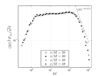
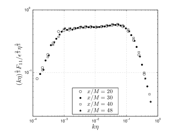
Figure 20: Compensated 1D energy spectra at four streamwise locations ($Re_{\lambda}=716,\,676,\,650,\,626$) at $U\approx 11ms^{-1}$, normalized by (a) $\overline{u^{2}}$ and $\ell\equiv 0.9\,u^{\prime 3}/\varepsilon$ (b) $\varepsilon$ and $\eta$. Data from Kang et al. (2003).

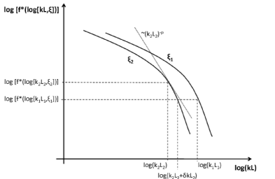
Figure 21: Sketch of two spectra at two streamwise positions $x=\xi_{1}$ and $x=\xi_{2}$ normalised with outer variables spreading at high frequency.

We outline the method by considering the dissipation range of the longitudinal spectrum and assuming the Kolmogorov scaling is correct, i.e. $F_{11}(k,x)=\varepsilon^{2/3}\eta^{5/3}f(k\eta)$, but this methodology is easily extendable to the energy containing range of the spectrum as well as to the case where the single-length-scaling is correct.

Consider two streamwise distances $x=\xi_{1}$ and $x=\xi_{2}$ and write $\eta_{1}=\eta(\xi_{1})$, $\eta_{2}=\eta(\xi_{2})$, $\lambda_{1}=\lambda(\xi_{1})$, $\lambda_{2}=\lambda(\xi_{2})$, $L_{1}=L_{u}(\xi_{1})$, $L_{2}=L_{u}(\xi_{2})$, $u^{\prime}_{1}=u^{\prime}(\xi_{1})$, $u^{\prime}_{2}=u^{\prime}(\xi_{2})$, $\varepsilon_{1}=\varepsilon(\xi_{1})$, $\varepsilon_{2}=\varepsilon(\xi_{2})$ for the Kolmogorov scales, Taylor micro-scales, integral scales, r.m.s. turbulence velocities and dissipation rates at these two locations. We take $\xi_{2}>\xi_{1}$ so that $Re_{L_{1}}\equiv u^{\prime}_{1}L_{1}/\nu>Re_{L_{2}}\equiv u^{\prime}_{2}L_{2}/\nu$.

Choose two wavenumbers $k_{1}$ and $k_{2}$ in the dissipation range such that $k_{1}\eta_{1}=k_{2}\eta_{2}$ and $f(k_{1}\eta_{1})=f(k_{2}\eta_{2})$ by assumption. If one would normalise the same spectra in this range using $u^{\prime 2}$ & $L_{u}$, the dependence of the normalised spectra on $x$ would explicitly resurface, i.e. $F_{11}(k,x)=u^{\prime 2}\,L_{u}\,f^{*}(kL_{u},x)$ (see figure 21). Since $\varepsilon=C_{\varepsilon}u^{\prime 3}/L_{u}$ with $C_{\varepsilon}$ independent of $x$ in the Richardson-Kolmogorov phenomenology, it follows that $L_{u}/\eta=C_{\varepsilon}^{1/4}Re_{L}^{3/4}$ and it is possible to show that

$$f^{*}(k_{1}L_{1},\xi_{1})=f^{*}(k_{2}L_{2},\xi_{2})\left(\frac{\eta_{1}}{L_{1}}\frac{L_{2}}{\eta_{2}}\right)^{5/3}=f^{*}(k_{2}L_{2},\xi_{2})\left(\frac{Re_{L_{2}}}{Re_{L_{1}}}\right)^{5/4}$$ (18)

and

$$k_{1}L_{1}=k_{2}L_{2}\left(\frac{\eta_{2}}{L_{2}}\frac{L_{1}}{\eta_{1}}\right)=k_{2}L_{2}\left(\frac{Re_{L_{1}}}{Re_{L_{2}}}\right)^{3/4},$$ (19)

so that $f^{*}(k_{1}L_{1},\xi_{1})\neq f^{*}(k_{2}L_{2},\xi_{2})$ and $k_{1}L_{1}\neq k_{2}L_{2}$.

We define the spectral spread which characterises the degree of non-collapse by the form $F_{11}=u^{\prime 2}L_{u}f^{*}(kL_{u})$ as

$$\Psi=\log(k_{1}L_{1})-\log(k_{2}L_{2}+\delta kL_{2}),$$ (20)

where $f^{*}(k_{1}L_{1},\xi_{1})=f^{*}(k_{2}L_{2}+\delta kL_{2},\xi_{2})$, see figure 21. There are two contributions to the spectral spread, one from the rescaling of the abscissas, $k_{1}L_{1}\neq k_{2}L_{2}$, and another from the rescaling of the ordinates. From $Re_{L_{1}}>Re_{L_{2}}$ and equations (18), (19) we know that $k_{1}L_{1}>k_{2}L_{2}$ and $f^{*}(k_{1}L_{1},\xi_{1})<f^{*}(k_{2}L_{2},\xi_{2})$ so that the two contributions to the spectral spread can actually in principle, cancel each other. However, the second contribution depends on the functional form of $f^{*}(kL_{u})$ and therefore it is not possible to quantify its spectral spread contribution without an analytical expression for $f^{*}(kL_{u},\xi)$. Nonetheless, as is shown below, we can estimate a bound for this contribution, so that in the end we can estimate a upper and lower bound for the expected spectral spread $\Psi$ characterising the degree of non-collapse by the alternative scaling.

The contribution to the spread $\Psi$ from the abscissa’s rescaling alone (which is the upper bound) is given by (using (19))

$$\Psi_{max}=\log(k_{1}L_{1})-\log(k_{2}L_{2})=\frac{3}{4}\log\left(\frac{Re_{L_{1}}}{Re_{L_{2}}}\right)=\frac{3}{2}\log\left(\frac{Re_{\lambda_{1}}}{Re_{\lambda_{2}}}\right).$$ (21)

(for the last equality, (6) was used to relate the integral scale to the Taylor micro-scale with $C_{\varepsilon}=Const$ from Richardson-Kolmogorov phenomenology).

The contribution to the spread $\Psi$ from the ordinate’s rescaling is measured as a fraction of the abscissa’s rescaling

$$\Phi\equiv\frac{\log(k_{2}L_{2}+\delta kL_{2})-\log(k_{2}L_{2})}{\log(k_{1}L_{1})-\log(k_{2}L_{2})},$$ (22)

so that $\Phi=0$ for $\delta kL_{2}=0$ (ordinate rescaling has no effect) and $\Phi=1$ for $\delta kL_{2}=k_{1}L_{1}-k_{2}L_{2}$ (ordinate rescaling cancels the abscissas rescaling). It is possible to show using a first order Taylor expansion in logarithmic coordinates that we can re-write the function $\Phi$ to leading order as

$$\Phi=-\frac{5}{3}\left(\left.\frac{\partial\,\log(f^{*}(\log(kL_{u}),\xi))}{\partial\,\log(kL_{u})}\right|_{kL_{u}=k_{2}L_{2}}\right)^{-1}.$$ (23)

Since the spectra in the dissipation range roll-off faster than any power law we can always find a high enough wavenumber $k_{t}(p)L_{u}$ for which the tangent of the spectrum (in logarithmic coordinates) is steeper than $(kL)^{-p}$ given an exponent $p$ (see figure 21). Consequently, for a given choice of $p$, we get an upper bound for $\Phi$ for wavenumbers above $k_{t}(p)L_{u}$ which is $\Phi_{max}=5/(3p)$. Therefore we can estimate a lower bound for the spectral spread as $\Psi_{min}=\Psi_{max}-\Phi_{max}$ and thus

$$\frac{3}{2}log\left(\frac{Re_{\lambda_{1}}}{Re_{\lambda_{2}}}\right)-\frac{5}{3p}<\Psi<\frac{3}{2}log\left(\frac{Re_{\lambda_{1}}}{Re_{\lambda_{2}}}\right).$$ (24)

In figure 20a we plot the $(kL_{u})^{-p}$ function with $p=4$ and it can be seen that for wavenumbers higher than $k_{t}L_{u}\approx 400$, the tangent of the spectra (in logarithmic coordinates) are steeper. Hence, according to (24), for $k_{t}L_{u}>400$ (taking into account the $Re_{\lambda}$ range of the data presented in figure 20a) the spectral spread will be around $5\%<\Psi<9\%$ of a decade, which can easily be confounded with scatter. Therefore, the apparent collapse observed in the spectra from the active-grid experiments of Kang et al. (2003) (see figure 20a) may be misleading as it is simply the result of a small range of $Re_{\lambda}$ variation during decay (from 716 to 637). Note that the same misleading collapse occurs in the low wavenumber range of the spectra plotted in figure 20b where the Kolmogorov inner variables were used for the normalisation.

We can repeat the exact same analysis for the case where the Richardson-Kolmogorov cascade is suppressed and assume the validity of $F_{11}(k,x)=u^{\prime 2}L_{u}f^{*}(kL_{u})$ and $L_{u}/\lambda\approx Const$. We can then carry out the same calculation as above to obtain the spectral spread $\Psi=\log(k_{1}\eta_{1})-\log(k_{2}\eta_{2}+\delta k\eta_{2})$ for $k_{1}L_{1}=k_{2}L_{2}$ when attempting to collapse the data with Kolmogorov variables. We would then obtain the same expression to quantify the spread contribution caused by the rescaling of the ordinates relative to the total spread, (22) with a suitably redefined $\Phi$ where the outer scales $L_{u}$ have been replaced by inner scales $\eta$. Note that spread of the high frequency spectra normalised by outer variables assuming that $F_{11}(k,x)=\varepsilon^{2/3}\eta^{5/3}f(k\eta)$ holds is the same as the spread of the high frequency spectra normalised by Kolmogorov inner variables assuming that $F_{11}(k,x)=u^{\prime 2}L_{u}f^{*}(kL_{u})$ holds. Hence, using $L_{u}\sim\lambda$, the spectral spread resulting from an attempt to collapse with Kolmogorov inner variables spectra which obey complete self-similarity is

$$\Psi=\log(k_{1}\eta_{1})-\log(k_{2}\eta_{2})=\frac{1}{2}\log\left(\frac{Re_{\lambda_{1}}}{Re_{\lambda_{2}}}\right)\hskip 2.84526pt.$$ (25)

It is interesting to observe that the rate of spread in this case is three times slower than the rate of spread when the Richardson-Kolmogorov cascade dominates and one tries to collapse with outer variables. Hence, the spectral spread observed in figure 14a is in agreement with the view that regular grid turbulence at the Reynolds numbers of this figure obeys Richardson-Kolmogorov interscale dynamics. However, the high-frequency behaviours in figures 14b, 15b and 15c fall within the uncertainty defined by (25) and we are therefore unable to conclude whether our fractal grid-generated turbulence obeys complete or incomplete self-similarity even though it is clear that $L_{u}\propto\lambda$ is a good approximation. By complete self-similarity we refer to the property that $F_{11}(k,x)=u^{\prime 2}L_{u}f^{*}(kL_{u})$ is exact at all frequencies and by incomplete self-similarity we refer to the property that deviations to $F_{11}(k,x)=u^{\prime 2}L_{u}f^{*}(kL_{u})$ can appear at the very highest frequencies. We stress that this does not imply Kolmogorov scaling even if these high frequencies may be collapsed by Kolmogorov inner variables for the simple reason that $L_{u}\propto\lambda$ and therefore $\varepsilon$ is not proportional to $u^{\prime 3}/L_{u}$.

References

- Antonia (2003) Antonia, R.A. 2003 On estimating mean and instantaneous turbulent energy dissipation rates with hot wires. Exp Therm Fluid Sci 27, 151–157.
- Antonia et al. (2003) Antonia, R.A., Smalley, RJ, Zhou, T., Anselmet, F. & Danaila, L. 2003 Similarity of energy structure functions in decaying homogeneous isotropic turbulence. J. Fluid Mech. 487, 245–269.
- Batchelor & Townsend (1948) Batchelor, GK & Townsend, AA 1948 Decay of isotropic turbulence in the initial period. Proc. Roy. Soc. A 193 (1035), 539–558.
- Batchelor (1953) Batchelor, G. K. 1953 The theory of homogeneous turbulence. Cambridge University Press, Cambridge.
- Burattini et al. (2005) Burattini, P., Lavoie, P. & Antonia, R.A. 2005 On the normalized turbulent energy dissipation rate. Phys. Fluids 17, 098103.
- Comte-Bellot & Corrsin (1966) Comte-Bellot, G. & Corrsin, S. 1966 The use of a contraction to improve the isotropy of grid-generated turbulence. J. Fluid Mech. 25 (04), 657–682.
- Corrsin (1963) Corrsin, S. 1963 Handbook der Physik. Springer, New York.
- Dimotakis (2000) Dimotakis, P. E. 2000 The mixing transition in turbulent flows. J. Fluid Mech. 409, 69–98.
- Ertunç et al. (2010) Ertunç, Ö., Özyilmaz, N., Lienhart, H., Durst, F. & Beronov, K. 2010 Homogeneity of turbulence generated by static-grid structures. J. Fluid Mech. 654 (1), 473–500.
- Freymuth (1977) Freymuth, P. 1977 Frequency response and electronic testing for constant-temperature hot-wire anemometers. J. Phys. E: Sci. Instrum. 10, 705.
- Frisch (1995) Frisch, U. 1995 Turbulence: The Legacy of AN Kolmogorov. Cambridge University Press, Cambridge.
- Gamard & George (2000) Gamard, S. & George, W. K. 2000 Reynolds number dependence of energy spectra in the overlap region of isotropic turbulence. Flow Turb. Comb. 63 (1), 443–477.
- Geipel et al. (2010) Geipel, P., Henry Goh, K. H. & Lindstedt, R. P. 2010 Fractal-Generated Turbulence in Opposed Jet Flows. Flow Turb. Comb. 85 (3–4), 397–419.
- George (1992) George, W. K. 1992 The decay of homogeneous isotropic turbulence. Phys. Fluids A 4 (7), 1492–1509.
- George & Wang (2009) George, W. K. & Wang, H. 2009 The exponential decay of homogeneous turbulence. Phys. Fluids 21, 025108.
- Goto & Vassilicos (2009) Goto, S. & Vassilicos, J. C. 2009 The dissipation rate coefficient of turbulence is not universal and depends on the internal stagnation point structure. Phys. Fluids 21, 035104.
- Helland & Van Atta (1977) Helland, K. N. & Van Atta, C. W. 1977 Spectral energy transfer in high reynolds number turbulence. J. Fluid Mech. 79 (02), 337–359.
- Hurst & Vassilicos (2007) Hurst, D. J. & Vassilicos, J. C. 2007 Scalings and decay of fractal-generated turbulence. Phys. Fluids 19, 035103.
- Ishida et al. (2006) Ishida, T., Davidson, P. A. & Kaneda, Y. 2006 On the decay of isotropic turbulence. J. Fluid Mech. 564, 455–475.
- Jayesh & Warhaft (1992) Jayesh & Warhaft, Z. 1992 Probability distribution, conditional dissipation, and transport of passive temperature fluctuations in grid-generated turbulence. Phys. Fluids A 4, 2292.
- Kahalerras et al. (1998) Kahalerras, H., Malecot, Y., Gagne, Y. & Castaing, B. 1998 Intermittency and reynolds number. Phys. Fluids 10, 910.
- Kang et al. (2003) Kang, H., Chester, S. & Meneveau, C. 2003 Decaying turbulence in an active-grid-generated flow and comparisons with large-eddy simulation. J. Fluid Mech. 480, 129–160.
- Kármán & Howarth (1938) Kármán, T. & Howarth, L. 1938 On the statistical theory of isotropic turbulence. Proc. Roy. Soc. A 164 (917), 192–215.
- Kinzel et al. (2011) Kinzel, M., Wolf, M., Holzner, M., Lüthi, B., Tropea, C. & Kinzelbach, W. 2011 Simultaneous two-scale 3D-PTV measurements in turbulence under the influence of system rotation. Exp Fluids 51 (1), 75–82.
- Kistler & Vrebalovich (1966) Kistler, A. L. & Vrebalovich, T. 1966 Grid turbulence at large reynolds numbers. J. Fluid Mech. 26, 37–47.
- Kolmogorov (1941) Kolmogorov, A. N. 1941 The local structure of turbulence in incompressible viscous fluid for very large Reynolds. CR Acad. Sci. URSS 30, 301.
- Krogstad & Davidson (2011) Krogstad, P. Å. & Davidson, P. A. 2011 Freely decaying, homogenous turbulence generated by multi-scale grids. J. Fluid Mech. 680, 417–434.
- Laizet & Vassilicos (2011) Laizet, S & Vassilicos, J. C. 2011 Dns of fractal-generated turbulence. Flow Turb. Combust. (to appear).
- Lavoie et al. (2007) Lavoie, P., Djenidi, L. & Antonia, RA 2007 Effects of initial conditions in decaying turbulence generated by passive grids. J. Fluid Mech. 585, 395–420.
- Lesieur (1997) Lesieur, M. 1997 Turbulence in Fluids. Dordrecht: Kluwer Academic.
- Lumley (1992) Lumley, W. K. 1992 Some comments on turbulence. Phys. Fluids A 4 (2), 203–211.
- Makita (1991) Makita, H. 1991 Realization of a large-scale turbulence field in a small wind tunne. Fluid Dyn. Res. 8.
- Mathieu & Scott (2000) Mathieu, J. & Scott, J. 2000 An Introduction to Turbulent Flows. Cambridge University Press, Cambridge.