Models of our Galaxy II

Abstract

Stars near the Sun oscillate both horizontally and vertically. In Paper I it was assumed that the coupling between these motions can be modelled by determining the horizontal motion without reference to the vertical motion, and recovering the coupling between the motions by assuming that the vertical action is adiabatically conserved as the star oscillates horizontally. Here we show that, although the assumption of adiabatic invariance works well, more accurate results can be obtained by taking the vertical action into account when calculating the horizontal motion. We use orbital tori to present a simple but fairly realistic model of the Galaxy’s discs in which the motion of stars is handled rigorously, without decomposing it into horizontal and vertical components. We examine the ability of the adiabatic approximation to calculate the model’s observables, and find that it performs perfectly in the plane, but errs slightly away from the plane. When the new correction to the adiabatic approximation is used, the density, mean-streaming velocity and velocity dispersions are in error by less than 10 per cent for distances up to $2.5\,{\rm kpc}$ from the Sun. The torus-based model reveals that at locations above the plane the long axis of the velocity ellipsoid points almost to the Galactic centre, even though the model potential is significantly flattened. This result contradicts the widespread belief that the shape of the Galaxy’s potential can be strongly constrained by the orientation of velocity ellipsoid near the Sun. An analysis of individual orbits reveals that in a general potential the orientation of the velocity ellipsoid depends on the structure of the model’s distribution function as much as on its gravitational potential, contrary to what is the case for Stäckel potentials. We argue that the adiabatic approximation will provide a valuable complement to torus-based models in the interpretation of current surveys of the Galaxy.

1 Introduction

Study of the structure of the Milky Way Galaxy is a major theme of contemporary astronomy. Our Galaxy is typical of the galaxies that dominate the current cosmic star-formation rate, so understanding it is of more than parochial interest. We believe that most of its mass is contributed by elementary particles that have yet to be directly detected, but we have only weak constraints on the spatial density and kinematics of these particles – we urgently need stronger constraints on them. The Cold-Dark-Matter (CDM) cosmogony provides a very persuasive picture of how a galaxy such as ours formed, and we need to know how accurately this theory predicts the structure of the Galaxy.

In view of these considerations, large resources have been invested over the last decade in massive surveys of the stellar content of the Galaxy. The rate at which data from this observational effort becomes available will increase at least through 2020. Models of the Galaxy will surely play a key role in extracting science from the data, because the Galaxy is a very complex object and every survey is subject to powerful observational biases. Consequently it is extremely hard to proceed in a model-independent way from observational data to physical understanding. We are likely to achieve the desired physical understanding by comparing observational data with the predictions of models.

It is useful to distinguish between kinematic and dynamic models. A kinematic model specifies the spatial density of stars and their kinematics at each point without asking whether a gravitational potential exists in which the given density distribution and kinematics constitute a steady state. Bahcall & Soneira (1984) pioneered kinematic models, and recent versions include Galaxia (Sharma et al., 2010). The science of constructing dynamical models is still in its infancy. The Besançon model (Robin et al., 2003) has a dynamical element to it in that in it the disc’s density profile perpendicular to the plane is dynamically consistent with the corresponding run of dispersion of velocities perpendicular to the plane. Schönrich & Binney (2009) and Binney (2010) (hereafter Paper I) offer models that are more thoroughly dynamical. These models adopt a plausible model of the Galaxy’s gravitational potential $\Phi(R,z)$, in which there are substantial contributions to the local acceleration from a disc, a bulge and a dark halo, all assumed to be axisymmetric. They assume that motion parallel to the plane is to some degree decoupled from motion perpendicular to the plane. Specifically, the vertical motion is governed by the time-dependent potential

$$\Psi_{z}(z;t)=\Phi[R(t),z]$$ (1)

where $R(t)$ is the radius at time $t$ that one obtains by assuming that the radial motion is governed by the one-dimensional effective potential

$$\Psi_{R}(R)=\Phi(R,0)+{L_{z}^{2}\over R^{2}}.$$ (2)

Paper I assumed that the time-dependence of the potential (1) is slow enough that the action $J_{z}$ of vertical motion is constant. It justified this assumption by referring to Figure 3.34 in Binney & Tremaine (2008) (hereafter BT08), which shows that the boundaries of one particular orbit are fairly well recovered by the adiabatic approximation (hereafter aa). In this paper we explore the validity of the aa much more extensively. Our other goal is to present a model of the Galactic disc that is not reliant on the aa. This model dispenses with the assumption that the $R$ and $z$ motions are decoupled by using numerically synthesised orbital tori.

The paper is organised as follows. In Section 2 the validity of the aa is tested on typical orbits. In Section 3 we explain the general principles of torus modelling and why we believe this technique will prove a valuable tool for the interpretation of observational data. We define the torus-based model of the Galactic discs that we will use to test the accuracy of observables obtained from the aa, and we summarise the methods used to extract observables when the model is based on (i) tori, and (ii) the adiabatic approximation. In Section 4 we compare the model’s observables with estimates of them obtained from the aa. In Section 5 we examine the tilt of the velocity ellipsoid near the Sun, which cannot be computed from the aa, and show that its long axis points towards the Galactic centre even though the potential is significantly flattened. Section 6 sums up and looks to the future. An appendix explains how some important Jacobians are calculated for a torus model.

Figure 1: Two orbits in the meridional plane of a Miyamoto-Nagai model with scale-length ratio $b/a=0.2$. In both cases the angular momentum about the symmetry axis is $L_{z}=\sqrt{GM/a}$, where $M$ is the model’s mass. In units of $\sqrt{GMa}$, the actions of the upper and lower orbits are $(J_{r},J_{z})=(0.109,0.067)$ and $(0.127,0.022)$. The numbers above each panel are the values of $J_{z}$ of obtained by following the motion of particles dropped from the upper left and upper right corners of the orbit in the one-dimensional potential $\Psi_{z}(z)=\Phi(R,z)-\Phi(R,0)$, and the corresponding vertical energies. The nearly straight full lines show the aa to the orbit when $J_{z}$ is set to the average of the values at top left and the radial action takes its true value. The dashed lines show the boundary yielded by the aa  when $L_{z}$ is replaced in the effective potential by $L_{z}+J_{z}$.

  

Figure 2: Surfaces of section $R/a=1.9,\,2.4$ and $3$ for the orbit shown in the top panel of Fig. 1. The points are for the numerically integrated orbit, while the curves are obtained from the aa.

2 validity of the adiabatic approximation

Each panel of Fig. 1 shows an orbit in the meridional plane in the gravitational potential of a Miyamoto-Nagai Galaxy model (Miyamoto & Nagai, 1975) with scale-length ratio $b/a=0.2$: Figure 2.7 of BT08 shows that this model has a prominent disc. From the Fourier transforms of the time series $R(t)$ $z(t)$ on these orbits (Binney & Spergel, 1984) we find that in units of $\sqrt{GMa}$ their actions are $(J_{r},J_{z})=(0.109,0.067)$ and $(0.127,0.022)$, respectively. One can also estimate the vertical actions $J_{z}$ of these orbits by dropping particles from points on their upper edges, and following their motion in the one-dimensional potential (1) with $R$ frozen at its current value – see equation (• ‣ 3.3) below. The numbers at top of each panel show the values obtained for $J_{z}$ in the same units when particles are dropped from the top left and top right corners of the orbit; the values are displaced from the true value by ${\,\mathrel{\mathchoice{\lower 2.9pt\vbox{\halign{$\m@th\displaystyle\hfil#\hfil$\cr<\crcr\sim\crcr}}}{\lower 2.9pt\vbox{\halign{$\m@th\textstyle\hfil#\hfil$\cr<\crcr\sim\crcr}}}{\lower 2.9pt\vbox{\halign{$\m@th\scriptstyle\hfil#\hfil$\cr<\crcr\sim\crcr}}}{\lower 2.9pt\vbox{\halign{$\m@th\scriptscriptstyle\hfil#\hfil$\cr<\crcr\sim\crcr}}}\,}}7\%$. The corresponding vertical energies $E_{z}$ are also shown at the top of each panel; they differ by more than a factor 2. Thus the aa does provide a fairly good guide to how the vertical motion is influenced by the radial motion.

The nearly straight full lines in Fig. 1 show the outlines of the approximate orbits that we obtain from the aa by setting $J_{r}$ to its true value and $J_{z}$ to the average of the values given at the top of the panel. The shape of each approximate orbit is reasonable, although the left and right edges are straight rather than curved, but the orbit is clearly displaced to smaller radii with respect to the true orbit. This difference reflects the fact that the vertical motion contributes to the centrifugal potential alongside the azimuthal motion. By assuming that the radial motion is governed by the effective potential (2) in which $L_{z}$ occurs rather than the total angular momentum $L$, we have under-estimated the centrifugal potential. Consequently, we predict that the orbit lives at smaller radii than it really does.

In a spherical potential, the total angular momentum is related to $L_{z}$ and $J_{z}$ by $L=|L_{z}|+J_{z}$ (e.g. BT08 §3.5.2) and the radial motion is governed by an effective potential in which the centrifugal component is $L^{2}/2r^{2}$, where $r^{2}=R^{2}+z^{2}$. Consequently, an obvious strategy for improving the predictions of the aa is to replace $L_{z}$ in the effective potential by $L+J_{z}$. The dashed lines in Fig. 1 show the effect of replacing $L_{z}$ by

$${\cal L}_{z}\equiv|L_{z}|+\gamma J_{z},$$ (3)

with $\gamma=1$. Both orbits are now quite closely modelled.

If we calculate the radial action of a given phase-space point $({\bf x},{\bf v})$ using $L_{z}$ rather than ${\cal L}_{z}$ in the effective potential, the value we obtain is too large when $({\bf x},{\bf v})$ lies near apocentre, because the star moves in an effective potential that has its minimum at a radius that is too small. Conversely, when $({\bf x},{\bf v})$ lies near pericentre, our estimate of $J_{r}$ is too small if we use $L_{z}$. Since the df decreases with increasing $J_{r}$, the use of the less accurate effective potential leads to phase-space points near pericentre being over-weighted relative to points near apocentre, and this in consequence shifts the predicted distribution in $v_{\phi}$ to large values. Hence, replacing $L_{z}$ in the effective potential with ${\cal L}_{z}$ for suitably chosen $\gamma$ can usefully improve the accuracy of results obtained with the aa.

The points in Fig. 2 show the consequents of the upper orbit of Fig. 1 in three surfaces of section that are obtained by noting $z$ and $p_{z}$ when the star crosses the line $R=\hbox{constant}$ in the meridional plane with $p_{R}>0$. The curves in each panel show the dependence of $p_{z}$ on $z$ along the one-dimensional orbit in the potential $\Phi(R,z)$ with $R$ fixed at the appropriate value when the action $J_{z}$ is set to the average of the values given above the top panel of Fig. 1. The agreement between the curves yielded by the aa and the numerical consequents is on the whole good. In the left and central panels we see that while the curves have reflection symmetry in $p_{z}=0$ the consequents do not. This is because the surface of section is for $p_{R}>0$, and when the star is moving outwards, it is likely to be moving upwards when $z>0$ and downwards when $z<0$. As we will discuss in Section 5, when a galaxy is formed out of such orbits, this $z$-dependent correlation between $p_{R}$ and $p_{z}$ causes the principal axes of the velocity ellipsoid to become inclined to the $R,z$ axes at $|z|>0$. The aa is unable to capture this aspect of the dynamics and will always yield a velocity ellipsoid that is aligned with the $R,z$ axes.

The panel on the extreme right shows that at large radii the aa underestimates the maximum height $z_{\rm max}$ reached by a star, although at most values of $z$ it predicts $p_{z}$ with good accuracy.

The analogue of Fig. 2 for the orbit shown in the lower panel of Fig. 1 shows smaller offsets between the numerical consequents and the predictions of the aa, because the latter works best for small vertical amplitudes.

With $v_{\rm t}$ denoting the tangential speed, the centrifugal potential is $v_{\rm t}^{2}/r^{2}$. In a separable potential, the time average of the $i$th component of velocity is related to the $i$th frequency and action by $\langle v_{i}^{2}\rangle=\Omega_{i}J_{i}$, so when we replace $v_{\rm t}^{2}$ by its time average the centrifugal potential becomes

$$\sim\Omega_{\phi}{|L_{z}|+(\Omega_{z}/\Omega_{\phi})J_{z}\over R^{2}+z^{2}}.$$ (4)

The standard aa underestimates the centrifugal potential by neglecting the term proportional to $J_{z}$ in the numerator, and partially compensates by neglecting the $z^{2}$ in the denominator. This neglect of $z^{2}$ must be responsible for the fact that we find the optimum value of $\gamma$ to be unity rather than $2$, which is a typical value of $\Omega_{z}/\Omega_{\phi}$ for disc stars at $R_{0}$ in plausible Galactic potentials. However, in an unrealistically flat potential, larger values of $\gamma$ prove optimal. For example, when the potential is that of a razor-thin exponential disc and there is no contribution from a bulge or a dark halo, we find $\gamma\simeq 1.9$ is required. Even in this case $\gamma$ is smaller than the typical value of $\Omega_{z}/\Omega_{\phi}$ on account of the neglect of $z^{2}$ in the denominator.

3 A model based on orbital tori

The classical approach to modelling globular clusters starts by positing an analytic form for the distribution function (df) and then calculating the density distribution and kinematics that are implied by this df. Thus globular clusters have been successfully modelled with dfs of the King–Michie form (e.g. BT08 §4.3). This approach can be extended to disc galaxies. For example Rowley (1988) modelled S0 galaxies with distribution functions of the form $f(E,L_{z})$, where $E$ and $L_{z}$ are, respectively, orbital energy per unit mass and and angular momentum per unit mass about the symmetry axis. Unfortunately, such a simple distribution function cannot successfully model the Galaxy, because it predicts equal velocity dispersions $\sigma_{R}$ and $\sigma_{z}$ in the radial and vertical directions, while observations show that $\sigma_{R}\simeq 1.7\sigma_{z}$ (e.g. Aumer & Binney, 2009). A successful df for the Galaxy must depend, explicitly or otherwise, on the vertical action $J_{z}$.

Given that the df will depend on two of an orbit’s three actions $J_{r}$, $J_{z}$ and $L_{z}$, substantial advantages arise from employing $J_{r}$ as the other argument of the df in place of $E$. For this reason Paper I studied Galaxy models in which each stellar component had a df that was an analytic function of the three actions. It used the aa to calculate observables from the df. The purpose of this section is to compare observables obtained in this way to those obtained without invoking the aa but instead using orbital tori.

3.1 General principles of torus modelling

Orbital tori are the three-dimensional surfaces in six-dimensional phase space on which individual orbits move. They are the building blocks from which Jeans’ theorem assures us that any equilibrium model can be built. Each torus is characterised by a set of three actions ${\bf J}=(J_{r},L_{z},J_{z})$ and therefore corresponds to a point in action space. We build a galaxy model by assigning a weight to each torus.

We obtain tori as the images of analytic tori under a canonical transformation. The tori used here are defined by the angle-action coordinates of the isochrone potential (e.g. BT08 §3.5). Given actions ${\bf J}$, the computer constructs a canonical transformation that maps the analytic torus with actions ${\bf J}$ into the required torus by adjusting the coefficients in a trial generating function so as to minimise the rms variation of the Galactic Hamiltonian on the image torus. Once this has been done, we have analytic expressions for the phase-space coordinates [${\bf x}({\mathchoice{\hbox{{\gkvecten\char 18\relax}}}{\hbox{{\gkvecten\char 18\relax}}}{\hbox{{\gkvecseven\char 18\relax}}}{\hbox{{\gkvecseven\char 18\relax}}}}),{\bf v}({\mathchoice{\hbox{{\gkvecten\char 18\relax}}}{\hbox{{\gkvecten\char 18\relax}}}{\hbox{{\gkvecseven\char 18\relax}}}{\hbox{{\gkvecseven\char 18\relax}}}})$] as functions of the angle variables $\theta_{i}$, which control the orbital phase. On a given torus, the phase-space coordinates $({\bf x},{\bf v})$ are $2\pi$-periodic functions of each $\theta_{i}$. The torus-fitting program also returns the values of the torus’s characteristic frequencies $\Omega_{i}$, so we can determine the motion of a star using ${\mathchoice{\hbox{{\gkvecten\char 18\relax}}}{\hbox{{\gkvecten\char 18\relax}}}{\hbox{{\gkvecseven\char 18\relax}}}{\hbox{{\gkvecseven\char 18\relax}}}}(t)={\mathchoice{\hbox{{\gkvecten\char 18\relax}}}{\hbox{{\gkvecten\char 18\relax}}}{\hbox{{\gkvecseven\char 18\relax}}}{\hbox{{\gkvecseven\char 18\relax}}}}(0)+{\bf\Omega}t$. For a fuller summary of how orbital tori are constructed and references to the papers in which torus dynamics was developed, see McMillan & Binney (2008).

Torus modelling is best understood as an extension of Schwarzschild modelling (Schwarzschild, 1979), which has been successfully used in many studies of the dynamics of external galaxies (e.g. Gebhardt et al., 2003; Krajnović et al., 2005). A Schwarzschild model is constructed by assigning weights to each orbit in a “library” of orbits. The orbit library is assembled by integrating the equations of motion in the given potential for a sufficient time, and noting the fraction of its time that the orbiting particle spends in each bin in the space of observables. Then a non-negative weight $w_{i}$ is chosen for each orbit such that the data are consistent with the model’s predictions. In torus modelling orbits are replaced by tori, which are essentially equivalence classes of orbits that differ from one another only in phase, and a Runge-Kutta integrator is replaced by the torus-fitting code. Whereas orbits are defined by their six-dimensional initial conditions, tori are defined by their actions ${\bf J}$.

Replacing numerically integrated orbits with orbital tori brings the following advantages

1. The phase-space density of orbits becomes known because tori have prescribed actions and the six-dimensional phase-space volume occupied by orbits with actions in ${\rm d}^{3}{\bf J}$ is $\tau=(2\pi)^{3}{\rm d}^{3}{\bf J}$. Knowledge of the phase-space density of orbits allows one to convert between orbital weights and the value taken by the df on an orbit.

2. On account of the above result, there is a clean and unambiguous procedure for sampling orbit space and relating the weights of individual tori to the value that the df takes on them – see below. The choice of initial conditions from which to integrate orbits for a library is less straightforward because the same orbit can be started from many initial conditions, and when the initial conditions are systematically advanced through six-dimensional phase space, the resulting orbits are likely at some point to cease exploring a new region of orbit space and start resampling a part of orbit space that is already represented in the library. On account of this effect, it is hard to relate the weight of an orbit to the value taken by the df on it (but see Häfner et al., 2000; Thomas et al., 2005).

3. There is a simple relationship between the distribution of stars in action space and the observable structure and kinematics of the model; as explained in §4.6 of BT08, the observable properties of a model change in a readily understood way when stars are moved within action space. The simple relationship between the observables and the distribution of stars in action space enables us to infer from the observables the form of the df $f({\bf J})$, which is nothing but the density of stars in action space.

4. From a torus one can readily find the velocities that a star on a given orbit can have when it reaches a given spatial point ${\bf x}$. By contrast a finite time series of an orbit is unlikely to exactly reach ${\bf x}$, and searching for the time at which the series comes closest to ${\bf x}$ is laborious. Moreover, several velocities are usually possible at a given location, and a representative point of closest approach must be found for each possible velocity.

5. An orbital torus is represented by of order 100 numbers while a numerically-integrated orbit is represented either by some thousands of six-dimensional phase-space locations, or by a similar number of occupation probabilities within a phase-space grid.

6. The numbers that characterise a torus are smooth functions of the actions ${\bf J}$. Consequently tori for actions that lie between the points of any action-space grid can be constructed by interpolation on the grid. Interpolation between time series is not practicable.

7. Schwarzschild and torus models are zeroth-order, time-independent models which differ from real galaxies by suppressing time-dependent structure, such as ripples around early-type galaxies (Malin & Carter, 1980; Quinn, 1984; Schweizer & Seitzer, 1992), and spiral structure or warps in disc galaxies. Since the starting point for perturbation theory is action-angle variables (e.g. Kalnajs, 1977), in the case of a torus model one is well placed to add time-dependent structure as a perturbation. Kaasalainen (1995) showed that classical perturbation theory works extremely well when applied to torus models because the integrable Hamiltonian that one is perturbing is typically much closer to the true Hamiltonian than in classical applications of perturbation theory (Gerhard & Saha, 1991; Dehnen & Gerhard, 1993; Weinberg, 1994), in which the unperturbed Hamiltonian arises from a potential that is separable (it is generally either spherical or plane-parallel).

3.2 Choice of the DF

For the comparison of results obtained with and without the aa it is appropriate to study a model that has a very simple df. Specifically we represent both the thin and the thick discs with a df that is quasi-isothermal in the sense of Paper I:

$$f(J_{r},L_{z},J_{z})=f_{\sigma_{r}}(J_{r},L_{z})\times{\nu_{z}\over 2\pi\sigma_{z}^{2}}\,{\rm e}^{-\nu_{z}J_{z}/\sigma_{z}^{2}},$$ (5)

where

$$f_{\sigma_{r}}(J_{r},L_{z})\equiv{\Omega\Sigma\over\pi\sigma_{r}^{2}\kappa}\bigg{|}_{R_{\rm c}}[1+\tanh(L_{z}/L_{0})]{\rm e}^{-\kappa J_{r}/\sigma_{r}^{2}}.$$ (6)

Here $\Omega(L_{z})$ is the circular frequency for angular momentum $L_{z}$, $\kappa(L_{z})$ is the radial epicycle frequency and $\nu(L_{z})$ is its vertical counterpart. $\Sigma(L_{z})=\Sigma_{0}{\rm e}^{-(R-R_{\rm c})/R_{\rm d}}$ is the (approximate) radial surface-density profile, where $R_{\rm c}(L_{z})$ is the radius of the circular orbit with angular momentum $L_{z}$. The factor $1+\tanh(L_{z}/L_{0})$ in equation (6) is there to effectively eliminate stars on counter-rotating orbits and the value of $L_{0}$ is unimportant provided it is small compared to the angular momentum of the Sun. In equations (5) and (6) the functions $\sigma_{z}(L_{z})$ and $\sigma_{r}(L_{z})$ control the vertical and radial velocity dispersions. The observed insensitivity to radius of the scaleheights of extragalactic discs motivates the choices

$$\sigma_{r}(L_{z}) = \sigma_{r0}\,{\rm e}^{q(R_{0}-R_{\rm c})/R_{\rm d}}$$

$$\sigma_{z}(L_{z}) = \sigma_{z0}\,{\rm e}^{q(R_{0}-R_{\rm c})/R_{\rm d}},$$ (7)

where $q=0.45$ and $\sigma_{r0}$ and $\sigma_{z0}$ are approximately equal to the radial and vertical velocity dispersions at the Sun. We take the df of the entire disc to be the sum of a df of the form (5) for the thin disc, and a similar df for the thick disc, the normalisations being chosen so that at the Sun the surface density of thick-disc stars is 23 per cent of the total stellar surface density. Table 1 lists the parameters of each component of the df.

Table 1: Parameters of the df.

Disc	$R_{\rm d}/\hbox{kpc}$	$\sigma_{r0}/\!\,{\rm km}\,{\rm s}^{-1}$	$\sigma_{z0}/\!\,{\rm km}\,{\rm s}^{-1}$	$L_{0}/\!\,{\rm kpc}\,{\rm km}\,{\rm s}^{-1}$
Thin	2.4	27	20	10
Thick	2.5	48	44	10

There are two main differences between the df we use here and that used in Paper I: (i) Paper I used the actual vertical frequency $\Omega_{z}({\bf J})$ in equation (5) while here we use the vertical epicycle frequency $\nu(L_{z})$. This substitution is necessary because for large ${\bf J}$, $\Omega_{z}$ tends to zero so fast that the product $\Omega_{z}J_{z}$ can decrease as $J_{z}\to\infty$, leading to unphysical results when $\Omega_{z}J_{z}$ appears in the df as the argument of an exponential. (ii) In the interests of simplicity the thin disc is here represented by a single quasi-isothermal component whereas in Paper I it was represented it by a sum of quasi-isothermals, one for stars of each age.

Any serious attempt to fit a real stellar catalogue must distinguish between stars of different ages, and different metallicities, because the colours and luminosities of stars are very much functions of age and metallicity, so the chances of a star entering a catalogue depend on its age and metallicity. Consequently, by lumping together all thin-disc stars regardless of age we forgo the opportunity to fit a real stellar catalogue in a detailed way. Nonetheless, we shall require our df to reproduce an observational density profile to demonstrate that even our unrealistically simple df has sufficient flexibility to reproduce given data to reasonable precision.

The physical properties of the model are jointly determined by the df and the gravitational potential $\Phi(R,z)$. Ultimately it will be necessary to require that the Galaxy’s df be consistent with $\Phi$ in the sense that the density of matter that the df predicts generates $\Phi$. However, before the question of dynamical self-consistency can be addressed, one must not only specify the df of dark matter (which is believed to contribute about half the gravitational force on the Sun) but also distinguish carefully between the masses of stars and their luminosities in the wavebands in which they are observed. In practice the latter can be done only if one has specified the Galaxy’s star-formation and metal-enrichment history. This enterprise goes far beyond the scope of the present paper; it will be addressed in subsequent papers in this series, which will explain the importance of comparing models to data in the space of observables, such as apparent magnitudes, parallaxes and proper motions, rather than the space of physical variables such as $({\bf x},{\bf v})$ used here. The purpose of this paper is merely to lay the foundations for such an exercise, which we expect to give first insights into the df of dark matter. Here we take the view that our df weights stars by their luminosity rather than their mass, and assume that $\Phi$ is the potential of Model 2 of Dehnen & Binney (1998) modified to have thin- and thick-disc scaleheights of $360\,{\rm pc}$ and $1\,{\rm kpc}$ (Table 2). In this model the disc contributes 60 per cent of the gravitational force on the Sun, with dark matter contributing most of the remaining force.

3.3 Modelling procedures

Together the df and the potential specify the probability density of stars in phase space. The simplest way to derive the model’s physical characteristics from this probability density is to obtain a discrete realisation of the probability density by Monte-Carlo sampling. The model’s physical characteristics are then obtained by binning the realisation’s stars. The df specified by equations (5) and (6) can be analytically integrated over $J_{z}$ and $J_{r}$ to obtain the marginal distribution in $L_{z}$, so we can obtain a discrete realisation of this df by successively sampling one-dimensional pdfs in $L_{z}$, $J_{r}$ and $J_{z}$. The results presented below are typically obtained with $\sim 200\,000$ tori.

Once we have a torus library, a discrete realisation of the Galaxy is obtained by repeatedly choosing a torus from the library at random, then choosing each angle variable uniformly within $(0,2\pi)$, and using the functions returned by the torus-generating software to to determine $({\bf x},{\bf v})$ from the given values of ${\bf J}$ and `.

When the aa is used, model construction proceeds rather differently: then given $({\bf x},{\bf v})$ one determines $J_{r}$ and $J_{z}$ by the following steps.

Table 2: Parameters of the potential

Component	$\Sigma(R_{0})/\,{\rm M}_{\odot}\,{\rm pc}^{-2}$	$R_{\rm d}/\hbox{kpc}$	$h/\!\,{\rm kpc}$	$R_{\rm m}/\!\,{\rm kpc}$
Thin	36.42	2.4	0.36	0
Thick	4.05	2.4	1	0
Gas	8.36	4.8	0.04	4

Component	$\rho/\!\,{\rm M}_{\odot}\,{\rm pc}^{-3}$	$q$	$\gamma$	$\beta$	$r_{0}/\!\,{\rm kpc}$	$r_{t}/\!\,{\rm kpc}$
Bulge	0.7561	0.6	1.8	1.8	1	1.9
Halo	1.263	0.8	$-2$	2.207	1.09	1000

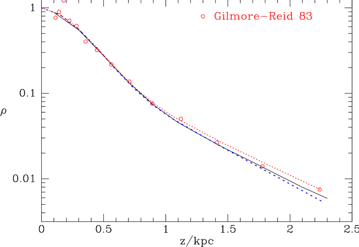
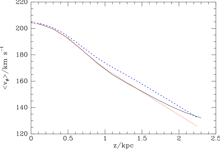
Figure 3: Top: density as a function of distance from the midplane at the solar radius. Bottom: mean streaming velocity as a function of distance from the midplane. The full black curves show the predictions of the full torus model; the blue curves are obtained from the aa with $\gamma=0$; the dotted red curves show the effect of setting $\gamma=1$.

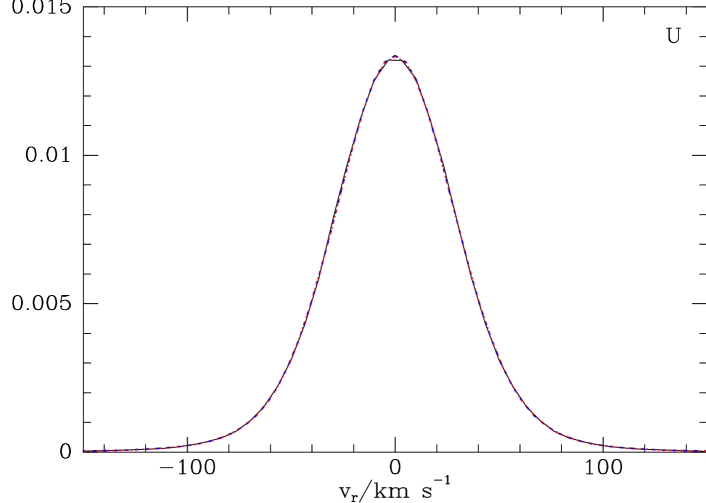
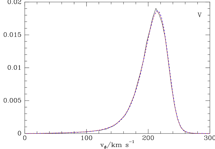
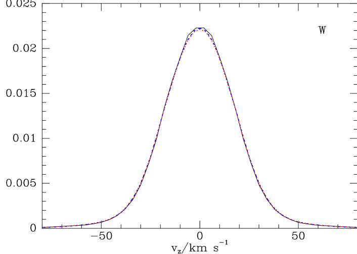
Figure 4: The distributions for local stars of the radial, azimuthal and vertical components of velocity after marginalising over the other two components. The full black curves are for the torus-based model while the broken curves are obtained using the aa with $\gamma=0$ (dashed blue) and $\gamma=1$ (dotted red). The curves overlie one another too closely to be clearly distinguishable.

• Evaluate the vertical and radial energies

  $$E_{z} = {\textstyle{1\over 2}}v_{z}^{2}+\Psi_{z}(z)$$

  $$E_{R} = {\textstyle{1\over 2}}v_{R}^{2}+\Psi_{R}(R),$$ (8)

  where $\Psi_{z}$ and $\Psi_{R}$ are defined by equations (1) and (2).

• Evaluate the actions from

  $$J_{z}={2\over\pi}\int_{0}^{z_{\rm max}}{\rm d}z\,v_{z}(E_{z},z)$$

  $$J_{r}={1\over\pi}\int_{R_{\rm p}}^{R_{\rm a}}{\rm d}R\,v_{R}(E_{R},R),$$ (9)

  where $z_{\rm max}$ is defined by $\Psi_{z}(z_{\rm max})=E_{z}$ and $R_{\rm a}$ and $R_{\rm p}$ are defined by $\Psi_{R}(R_{i})=E_{R}$.

These steps make it straightforward to evaluate the df at an arbitrary point $({\bf x},{\bf v})$, and thus derive the model’s physical properties by numerically integrating the df, times any power of $v_{i}$, over velocity space. The quantities such as stellar number density $\nu({\bf x})$ and velocity dispersion $\langle v_{z}\rangle^{1/2}({\bf x})$ are then continuous functions of their arguments. In the absence of the aa, an iterative procedure such as that described by McMillan & Binney (2008) is required to determine ${\bf J}({\bf x},{\bf v})$, and the torus-modeeling procedure avoids this procedure by choosing ${\bf J}$ not $({\bf x},{\bf v})$. The price we pay for starting with ${\bf J}$ is discreteness, and the necessity of estimating $\nu({\bf x})$, etc, by binning stars.

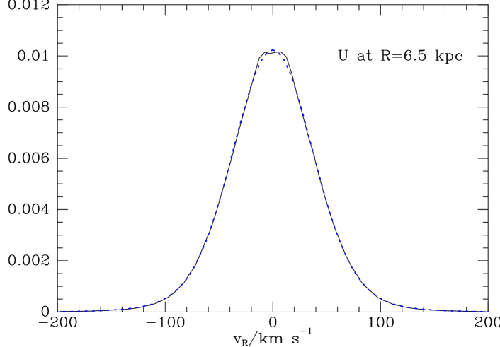
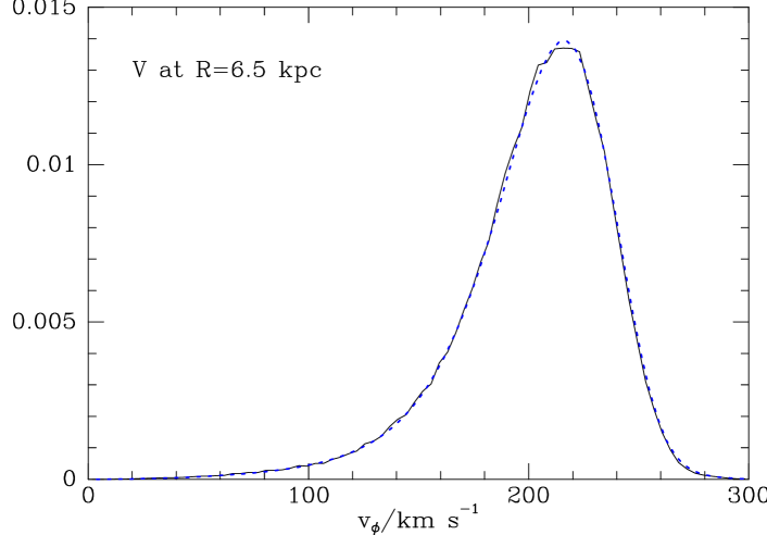
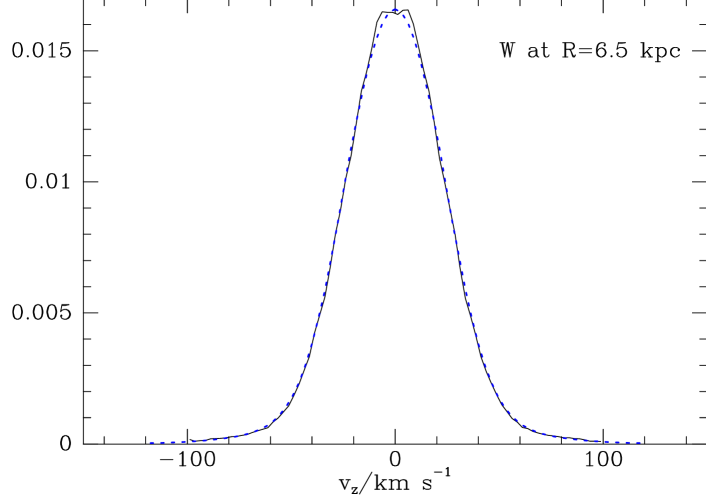
Figure 5: As Fig. 4 except for a volume that lies in the plane at $R=6.5\,{\rm kpc}$.

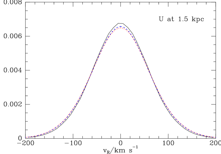
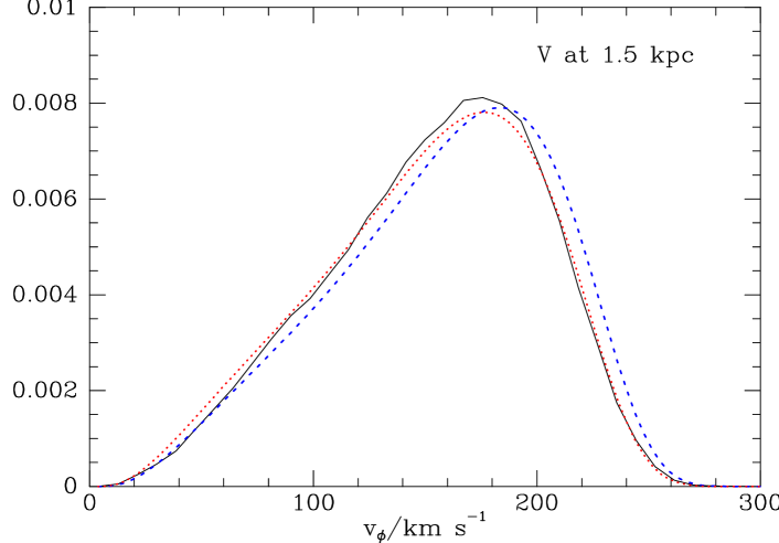
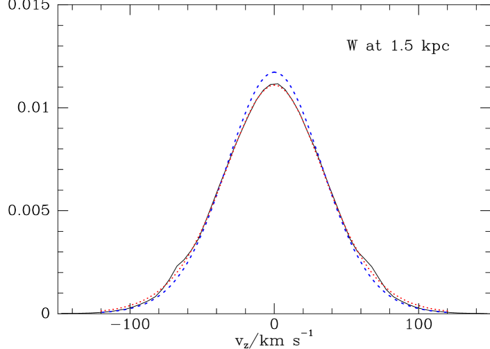
Figure 6: As Fig. 4 except for a volume that is $1.5\,{\rm kpc}$ from the plane. The dotted red curves are for the aa with $\gamma=1$ rather than 0, shown by the broken blue curves.

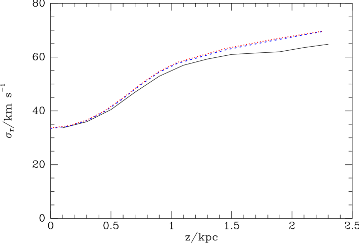
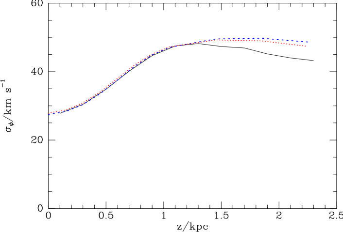
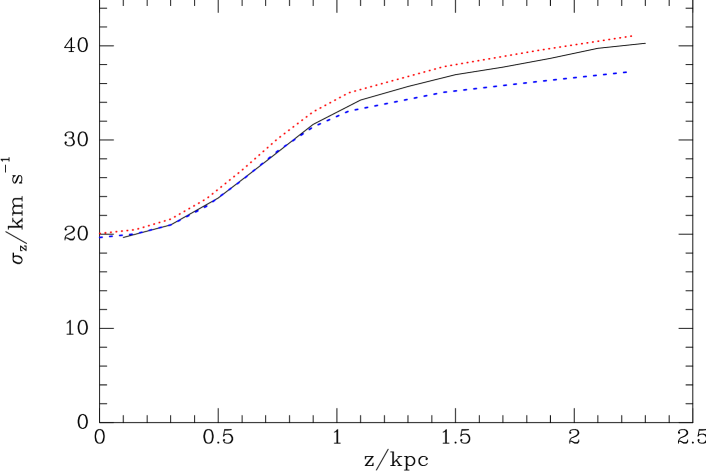
Figure 7: The radial, azimuthal and vertical velocity dispersions as functions of distance from the midplane. The full black curve shows results from the torus model, while the dashed blue line is obtained using the aa with $\gamma=0$; the dotted red curves show the effect of setting $\gamma=1$.

4 Comparisons

Fig. 3 shows the density of stars (upper panel) and the mean-streaming velocity (lower panel) as functions of $|z|$ at the solar radius. The full curves show results from the torus model, while the dashed and dotted curves show results obtained from the aa using two values of the parameter $\gamma$ defined by eq. (3): $\gamma=0$ (dotted red) and $\gamma=1$ (dashed blue). Also shown in the upper panel are the seminal data points of Gilmore & Reid (1983), which led to the identification of the thick disc. Since our df provides a reasonable fit to these points, it may be close to the actual df for turnoff stars. The aa recovers the density profile of the torus model to good accuracy for either value of $\gamma$.

The lower panel in Fig. 3 shows how the mean streaming speed $\left\langle v_{\phi}\right\rangle$ is predicted to fall with $|z|$. The agreement between the torus model and the model based on the aa with $\gamma=1$ (dotted red) is excellent for $|z|\la 1.6\,{\rm kpc}$ but at larger heights the aa has a systematic tendency to under-estimate $\left\langle v_{\phi}\right\rangle$. On account of the problem discussed in Section 2 apropos Fig. 1, the aa with $\gamma=0$ over-estimates the mean-streaming speed by a few $\!\,{\rm km}\,{\rm s}^{-1}$ for $|z|{\,\mathrel{\mathchoice{\lower 2.9pt\vbox{\halign{$\m@th\displaystyle\hfil#\hfil$\cr>\crcr\sim\crcr}}}{\lower 2.9pt\vbox{\halign{$\m@th\textstyle\hfil#\hfil$\cr>\crcr\sim\crcr}}}{\lower 2.9pt\vbox{\halign{$\m@th\scriptstyle\hfil#\hfil$\cr>\crcr\sim\crcr}}}{\lower 2.9pt\vbox{\halign{$\m@th\scriptscriptstyle\hfil#\hfil$\cr>\crcr\sim\crcr}}}\,}}0.7\,{\rm kpc}$.

Fig. 4 shows the distributions of the radial ($U$), tangential ($V$) and vertical ($W$) components of velocity in a small volume akin to the solar neighbourhood. Since the full black curves from the torus model coincide with the dashed blue curves from the aa with $\gamma=0$, the aa reproduces the torus results to high precision. The results obtained on setting $\gamma=1$ are plotted as a dotted red curve but overlie the other curves too closely to be clearly distinguishable. Fig. 5 shows that the aa is equally successful in recovering the distributions of $U$, $V$ and $W$ at a smaller Galactocentric radius, $6.5\,{\rm kpc}$. The insensitivity to $\gamma$ of the velocity distribution in the plane arises because these distributions are dominated by rather nearly circular orbits, and for these orbits $J_{z}$ is so much smaller than $L_{z}$ that adding $J_{z}$ to $L_{z}$ barely changes the numerical value.

Fig. 6 shows the $U$, $V$ and $W$ distributions at $R=8\,{\rm kpc}$ and $1.5\,{\rm kpc}$ away from the midplane. Systematic differences between the predictions of the aa and the results of the full torus model are now evident. For either value of $\gamma$, the aa yields a distribution of $U$ that is slightly too broad. When $\gamma=0$, the aa gives a distribution in $W$ (dashed blue curve) that is too sharply peaked, but this fault is nicely corrected by setting $\gamma=1$ (dotted red curve) because increasing $\gamma$ moves orbits of given $L_{z}$ outwards, and by virtue of equation (3.2), the smaller an orbit’s value of $L_{z}$, the faster it is likely to move vertically. As expected, with $\gamma=0$ the aa yields a distribution in $V$ that is offset from that of the full torus model by $\sim 8\,{\rm km}\,{\rm s}^{-1}$ towards higher velocities (dashed blue curve). This offset is largely cured by setting $\gamma=1$ (dotted red curve).

Fig. 7 shows the variation with $|z|$ of the radial, tangential and vertical velocity dispersions. The two planar velocity dispersions are accurately reproduced for $|z|\la 1.3\,{\rm kpc}$. At greater heights the aa over-estimates the dispersions, most strikingly so in the case of $\sigma_{\phi}$. The excessive value of $\sigma_{\phi}$ is clearly associated with the tendency of the red curve in the middle panel of Fig. 6 to lie above the black one at $v_{\phi}\sim 50\,{\rm km}\,{\rm s}^{-1}$. As the top and middle panels of Fig. 6 suggest, $\langle v_{R}^{2}\rangle^{1/2}$ and $\langle(v_{\phi}-\langle v_{\phi}\rangle)^{2}\rangle^{1/2}$ are at any height remarkably insensitive to the value of $\gamma$.

From the bottom panel of Fig. 6 we anticipate that increasing $\gamma$ will increase $\langle v_{z}^{2}\rangle$ at large $|z|$ and indeed the bottom panel of Fig. 7 shows that increasing $\gamma$ from zero to unity increases $\sigma_{z}$ at all $z$, but particularly at large $z$. This result arises because increasing $\gamma$ shifts orbits with large $J_{z}$ outwards, and since $f({\bf J})$ is a strongly decreasing function of $|{\bf J}|$, this outwards shift raises the density of stars with large $J_{z}$ at a given location. At $|z|\ga 1\,{\rm kpc}$ setting $\gamma=1$ increases the accuracy of $\sigma_{z}$, while at smaller values of $|z|$, a slight deterioration in accuracy results. The bottom panel of Fig. 6 hints that the full curve in Fig. 7 may lie slightly too low as a result of poor sampling by the torus model of orbits with large $|v_{z}|$, so the results from the aa with $\gamma=1$ may be more accurate than appears to be the case.

Figure 8: Three effective potentials for the orbit in the Galaxy model that has actions $(J_{r},L_{z},J_{z})=(0.05,1,0.05)$ times the angular momentum of the circular orbit at $R_{0}$. This orbit extends to $3\,{\rm kpc}$ above the plane. The dotted and dashed curves show the naive effective potential (2) with $L_{z}$ replaced by $|L_{z}|+\gamma J_{z}$ and $\gamma=0$ in the dotted case and $\gamma=1$ in the dashed case. The full curve shows the effective potential derived from a time-average of the radial force.

The dotted and dashed curves in Fig. 8 show the effective potential (2) for a typical solar-neighbourhood orbit when $\gamma=0$ and $\gamma=1$, respectively. The full curve shows an effective potential for this orbit that was obtained by first evaluating the time-average of $\partial\Phi/\partial R-L_{z}^{2}/R^{3}$ at each value of $R$ visited by the orbit, and then integrating the resulting function of $R$. We see that with $L_{z}$ replaced by $|L_{z}|+J_{z}$ the simple effective potential (2) provides a good fit to the effective potential obtained by time-averaging the radial force as a function of $R$.

Figure 9: The variation of the angle of tilt of the velocity ellipsoid with respect to the plane versus the angle $\arctan(|z|/R)$ between the plane and the line of sight from ($R,z$) to the Galactic centre. Since the full curve tracks the dotted line, the long velocity ellipsoid points almost straight at the Galactic centre.

Figure 10: The distribution of the ratio $u_{z}/u_{R}$ that gives the direction of a principal axis of the contribution of each torus to the velocity ellipsoid at the point $(R,z)=(R_{0},1.5\,{\rm kpc})$. The full histogram weights each torus equally, while the dotted one weights them in proportion to their contributions to the density at the given point. Even the latter distribution is wide, so the orientation of the velocity ellipsoid depends quite sensitively on the weights assigned to orbits by the df.

5 Tilt of the velocity ellipsoid

A popular diagnostic of the Galaxy’s gravitational potential is the way in which the principal axes of the velocity ellipsoid tilt as one moves away from the plane (Siebert et al., 2008; Smith et al., 2009). As stated above, this phenomenon lies beyond the scope of the aa, but it can be determined from the torus model. Fig. 9 shows that this angle is nearly equal to the angle $\arctan(|z|/R)$ between the plane and the line of sight from ($R,z$) to the Galactic centre. That is, in the vicinity of the Sun, the longest axis of the velocity ellipsoid is almost parallel to the radial vector ${\bf r}$.

This behaviour is that expected in a spherical potential, and Smith et al. (2009) argue that alignment of the velocity ellipsoid with spherical coordinates implies that the potential is spherically symmetric. Our assumed gravitational potential is far from spherical because roughly half the radial force at the Sun is contributed by the disc, and the dark halo is itself flattened (axis ratio $0.8$). The aspherical nature of the potential is reflected in the fact that the distribution of frequency ratios $\Omega_{z}/\Omega_{\phi}$ of the model’s tori, has a median close to 2, while in a spherical potential this ratio is inevitably unity.

Although our model is not strictly speaking a counter example to the assertion of Smith et al. (2009) because we have established only that the velocity ellipsoid is approximately aligned with spherical coordinates in the region around the Sun, it does suggest that one should examine more closely the reasoning in that paper.

A key step in its argument is the assertion that if the df is an even function of $v_{r}^{2}$, then the isolating integrals that constrain individual orbits are also. If the isolating integrals have this property, then the velocity ellipsoid provided by any df will be aligned with spherical coordinates. In particular the df $f({\bf J})=\delta({\bf J}-{\bf J}_{0})$ corresponding to a single orbit will be radially aligned, so the matrix $\langle v_{i}v_{j}\rangle_{\bf x}$ will be diagonal in spherical coordinates, where $\langle.\rangle_{\bf x}$ implies the time average over instants when the star lies in some small volume around ${\bf x}$.

As Fig. 1 illustrates, for stars on standard orbits in the meridional plane, four velocities are possible at a given point. Let these velocities be $\pm{\bf v}_{1}$ and $\pm{\bf v}_{2}$. By time-reversal symmetry, the probability that ${\bf v}_{1}$ occurs is inevitably equal to the probability that $-{\bf v}_{1}$ occurs, and similarly for $\pm{\bf v}_{2}$. However, it turns out that $\pm{\bf v}_{1}$ may occur more or less often than $\pm{\bf v}_{2}$. In fact the probability of occurrence of ${\bf v}_{i}$ is proportional to the Jacobian $\partial({\mathchoice{\hbox{{\gkvecten\char 18\relax}}}{\hbox{{\gkvecten\char 18\relax}}}{\hbox{{\gkvecseven\char 18\relax}}}{\hbox{{\gkvecseven\char 18\relax}}}})/\partial({\bf x})$, which is a non-trivial function of `, but one that can be determined for a numerically constructed torus (see Appendix A). The four possible velocities at ${\bf x}$ correspond to the four values of ` that bring the star to the given point ${\bf x}$, and the values $p_{1}$ and $p_{2}$ taken by $\partial({\mathchoice{\hbox{{\gkvecten\char 18\relax}}}{\hbox{{\gkvecten\char 18\relax}}}{\hbox{{\gkvecseven\char 18\relax}}}{\hbox{{\gkvecseven\char 18\relax}}}})/\partial({\bf x})$ at these values of ` depend on whether ${\bf v}$ is $\pm{\bf v}_{1}$ or $\pm{\bf v}_{2}$. Clearly we have

$$\langle v_{i}v_{j}\rangle_{\bf x}={p_{1}v_{1i}v_{1j}+p_{2}v_{2i}v_{2j}\over p_{1}+p_{2}}.$$ (10)

Let ${\bf u}$ be the eigenvector of this matrix that lies closest to the ${\bf r}$ direction. Fig. 10 shows for the point $(R,z)=(8,1.5)\,{\rm kpc}$ the distribution of the ratio $u_{z}/u_{R}$. The full histogram shows the distribution when each torus is given equal weight, while the dotted histogram shows the distribution when tori are correctly weighted by the contributions that they make to the stellar density at the given point. (Although the density of sampling in action space ensures that all tori make equal contributions to the stellar mass of the entire Galaxy, every torus has its own way of spreading its mass in space.) We see that the distribution of orientations of individual contributions to the velocity ellipsoid is quite broad, even when the tori are correctly weighted. An examination of the dependence of $u_{z}/u_{R}$ on $J_{z}$ reveals that orbits with larger values of $J_{z}$ make contributions that are aligned with ${\bf r}$, while it is orbits with small $J_{z}$ that sometimes make contributions that are aligned nearly parallel to the plane. Since the df specifies the relative weight of these variously oriented contributions, it controls the orientation of the final velocity ellipsoid at least as much as does the gravitational potential. Consequently, only limited inferences about the nature of the potential can be drawn from observations of the velocity ellipsoid yielded by the df that the Galaxy happens to have.

The widespread belief that the shape of the potential can be inferred from the orientation of the velocity ellipsoid probably arises from studies of models that have Stäckel potentials. For these potentials the Hamilton-Jacobi equation separates in an appropriate coordinate system $(u,v)$, and the canonically conjugate momenta are functions of one coordinate only: $p_{u}(u)$, $p_{v}(v)$ (e.g. BT08 §3.5.3). Consequently, the coordinate directions are bisectors of the angles between ${\bf v}_{1}$ and ${\bf v}_{2}$. Moreover, it turns out that for these potentials, $\partial({\mathchoice{\hbox{{\gkvecten\char 18\relax}}}{\hbox{{\gkvecten\char 18\relax}}}{\hbox{{\gkvecseven\char 18\relax}}}{\hbox{{\gkvecseven\char 18\relax}}}})/\partial({\bf x})$ is the same for all four values of ` so the coordinate directions are the eigenvectors of $\langle v_{i}v_{j}\rangle_{\bf x}$ for every orbit that reaches ${\bf x}$. Consequently, the velocity ellipsoid has to be oriented with the coordinate directions regardless of how orbits are weighted. In a general potential, there is no universal coordinate system that describes the alignment of the egenvectors of $\langle v_{i}v_{j}\rangle_{\bf x}$, and the orientation of the final velocity ellipsoid very much depends on how orbits are weighted.

6 conclusions

Dynamical models of the Milky Way will play an key role in the scientific exploitation of data from large surveys that are currently being undertaken. Models that are based on Jeans’ theorem should be the most powerful tools for extracting science from data, and amongst such models those that express the df as a function of the actions enjoy some very important advantages.

The major obstacle to the use of Jeans’ theorem in the context of the Galaxy is the lack of analytic expressions for three independent isolating integrals. Paper I presented models that use approximate expressions for the actions that rely on the adiabatic invariance of the vertical action $J_{z}$. In Section 2 we tested the validity of this adiabatic approximation (aa) by numerically integrating typical orbits. We found that the orbits’ vertical dynamics is reproduced by the aa to remarkably good accuracy, but the motion in the plane is less accurately recovered because the naive aa under-estimates the strength of the centrifugal potential. This defect leads to the radial action derived for a given phase-space point $({\bf x},{\bf v})$ being over-estimated when the point lies near apocentre, and under-estimated when it lies near pericentre. Since $v_{\phi}$ is small at apocentre and large near pericentre and the df is a declining function of $J_{r}$, the defect leads to the mean-streaming velocity $\langle v_{\phi}\rangle$ being over-estimated. The problem can be largely resolved by replacing $L_{z}$ in the centrifugal potential by $|L_{z}|+\gamma J_{z}$ with $\gamma$ a number of order unity.

The more strongly flattened the potential is, the more accurate the aa becomes and the larger the value of $\gamma$ needs to be. For example, in the extreme case of vanishing dark halo $\gamma=1.9$ works well.

In Section 3 we explained how to build a model Galaxy using orbital tori. Torus modelling is best considered an extension of Schwarzschild modelling, which has long been a standard tool for the interpretation of data for external galaxies, both in connection with searches for massive black holes and attempts to understand how early-type galaxies were assembled. Torus modelling is a more powerful technique principally because (i) it enables us to quantify orbits by the values taken on them of essentially unique and physically easily understood isolating integrals, and (ii) it makes it easy to determine at what velocities a star will pass through any spatial point. We presented a df of exceptional simplicity, which generates a reasonably realistic model of the Galaxy’s discs.

In Section 4 we examined in some detail observable quantities in this model when they are calculated from either the full torus machinery, or from the aa. We showed that in the plane, at both $R_{0}$ and $R=6.5\,{\rm kpc}$, the distributions of all three components of velocity are reproduced to high accuracy by the aa, regardless of whether $\gamma$ is set to zero or unity. Away from the plane the velocity distribution is sensitive to the weights of orbits that have relatively large values of $J_{z}$, with the consequence that it matters whether the centrifugal potential contains $L_{z}$ or $|L_{z}|+\gamma J_{z}$, and we find materially better fits to the distributions of both $v_{\phi}$ and $v_{z}$ when $\gamma=1$ rather than zero.

Regardless of the value of $\gamma$, the aa predicts a value for $\langle v_{R}\rangle^{1/2}$ that exceeds the true value by an amount that grows with $|z|$, being $\sim 3.4$ per cent at $|z|=1.5\,{\rm kpc}$. The aa yields a value of $\sigma_{\phi}$ that lies very close to the true value for $|z|<1.3\,{\rm kpc}$, but exceeds the true value by $\sim 10$ percent at $|z|=2\,{\rm kpc}$ because the true value declines with $|z|$ at $|z|>1.3\,{\rm kpc}$, whereas that obtained from the aa does not. With $\gamma=1$ the aa yields a value for $\langle v_{z}\rangle^{1/2}$ that lies within 3 percent of the true value right up to $|z|=2.3\,{\rm kpc}$.

The aa inevitably predicts that the velocity ellipsoid has two axes parallel to the plane, so we must turn to the full torus model to discover how the velocity ellipsoid tilts as one moves away from the plane. We find that its longest axis points quite close to the Galactic centre. This result emerges through averaging the quite disparate contributions of individual tori. Consequently it reflects the structure of the df as much as the gravitational potential.

From a computational perspective, the aa is extremely convenient, both because it does not require specialised torus-generating code, and because it yields ${\bf J}$ from $({\bf x},{\bf v})$ rather than $({\bf x},{\bf v})$ from ${\bf J}$. Consequently, a model’s observables can be obtained by integrating over velocity space, just as traditionally we have obtained the observables of models with dfs of the form $f(E)$ and $f(E,L)$. While McMillan & Binney (2008) showed that it is possible to determine ${\bf J}$ from $({\bf x},{\bf v})$, the procedure used is iterative and time-consuming, so for this paper observables were estimated by binning the particles of a discrete realisation obtained by Monte-Carlo sampling the df. Even this procedure is computationally expensive when enough samples are drawn to make Poisson noise negligible, so it is very useful to be able to obtain good approximations to ${\bf J}({\bf x},{\bf v})$ from the aa, and we anticipate that the aa will be widely used in the interpretation of observations of the Galaxy.

Paper I and the present paper represent two small steps towards the kind of Galaxy modelling apparatus that should available before a preliminary Gaia Catalogue appears in the second half of this decade. The next big step is to carry the predictions of models into the space of observables – such as apparent magnitudes, parallaxes and proper motions – and then to explore how tightly the df of stars can be constrained by data of varying extent and precision. This step is crucial because distance uncertainties propagate from observables such as magnitudes and proper motions to correlated errors in physical quantities such as stellar masses and velocities. We hope to report on this work soon.

Appendix A: Evaluating Jacobians

The observables of individual orbits can be obtained from the df $f({\bf J})=\delta({\bf J}-{\bf J}_{0})$, where ${\bf J}_{0}$ gives the orbits actions. Then

$$\langle v_{i}v_{j}\rangle_{\bf x} = \int{\rm d}^{3}{\bf v}\,v_{i}v_{j}f({\bf J})=\int{\rm d}^{3}{\bf J}\,\left.{\partial({\bf v})\over\partial({\bf J})}\right|_{\bf x}v_{i}v_{j}\delta({\bf J}-{\bf J}_{0})$$ (11)

$$= \sum_{i}\left(\left.{\partial({\bf v})\over\partial({\bf J})}\right|_{\bf x}v_{i}v_{j}\right)_{{\mathchoice{\hbox{{\gkvecten\char 18\relax}}}{\hbox{{\gkvecten\char 18\relax}}}{\hbox{{\gkvecseven\char 18\relax}}}{\hbox{{\gkvecseven\char 18\relax}}}}_{i}},$$

where ${\mathchoice{\hbox{{\gkvecten\char 18\relax}}}{\hbox{{\gkvecten\char 18\relax}}}{\hbox{{\gkvecseven\char 18\relax}}}{\hbox{{\gkvecseven\char 18\relax}}}}_{i}$ are the phases that bring the star to ${\bf x}$.

Since both the $({\bf x},{\bf v})$ and $({\mathchoice{\hbox{{\gkvecten\char 18\relax}}}{\hbox{{\gkvecten\char 18\relax}}}{\hbox{{\gkvecseven\char 18\relax}}}{\hbox{{\gkvecseven\char 18\relax}}}},{\bf J})$ systems are canonical, there exists a generating function $G({\bf J},{\bf x})$ for the transformation $({\bf x},{\bf v})\leftrightarrow({\bf J},{\mathchoice{\hbox{{\gkvecten\char 18\relax}}}{\hbox{{\gkvecten\char 18\relax}}}{\hbox{{\gkvecseven\char 18\relax}}}{\hbox{{\gkvecseven\char 18\relax}}}})$. So

$$\theta_{i}={\partial G\over\partial J_{i}}\quad;\quad v_{j}={\partial G\over\partial x_{j}}$$ (12)

Differentiating again

$$\left({\partial\theta_{i}\over\partial x_{j}}\right)_{\bf J}={\partial^{2}G\over\partial x_{j}\partial J_{i}}=\left({\partial v_{j}\over\partial J_{i}}\right)_{\bf x}.$$ (13)

Taking determinants

$$\left.{\partial({\mathchoice{\hbox{{\gkvecten\char 18\relax}}}{\hbox{{\gkvecten\char 18\relax}}}{\hbox{{\gkvecseven\char 18\relax}}}{\hbox{{\gkvecseven\char 18\relax}}}})\over\partial({\bf x})}\right|_{\bf J}=\left.{\partial({\bf v})\over\partial({\bf J})}\right|_{\bf x}.$$ (14)

The Jacobian on the left is the orbit’s probability density in real space because the amount of time a star spends in a region of angle space is proportional to its volume, ${\rm d}^{3}{\mathchoice{\hbox{{\gkvecten\char 18\relax}}}{\hbox{{\gkvecten\char 18\relax}}}{\hbox{{\gkvecseven\char 18\relax}}}{\hbox{{\gkvecseven\char 18\relax}}}}$. It makes good physical sense that the Jacobian in equation (11) is the orbit’s probability density.

With toy variables distinguished from true ones by a superscript T, the generating function of the transformation $({\mathchoice{\hbox{{\gkvecten\char 18\relax}}}{\hbox{{\gkvecten\char 18\relax}}}{\hbox{{\gkvecseven\char 18\relax}}}{\hbox{{\gkvecseven\char 18\relax}}}},{\bf J})\leftrightarrow({\mathchoice{\hbox{{\gkvecten\char 18\relax}}}{\hbox{{\gkvecten\char 18\relax}}}{\hbox{{\gkvecseven\char 18\relax}}}{\hbox{{\gkvecseven\char 18\relax}}}}^{(\rm T)},{\bf J}^{(\rm T)})$ between true and toy angle-action variables is

$$S({\bf J},{\mathchoice{\hbox{{\gkvecten\char 18\relax}}}{\hbox{{\gkvecten\char 18\relax}}}{\hbox{{\gkvecseven\char 18\relax}}}{\hbox{{\gkvecseven\char 18\relax}}}}^{(\rm T)})={\bf J}\cdot{\mathchoice{\hbox{{\gkvecten\char 18\relax}}}{\hbox{{\gkvecten\char 18\relax}}}{\hbox{{\gkvecseven\char 18\relax}}}{\hbox{{\gkvecseven\char 18\relax}}}}^{(\rm T)}+\sum_{\bf n}s_{\bf n}({\bf J})\sin({\bf n}\cdot{\mathchoice{\hbox{{\gkvecten\char 18\relax}}}{\hbox{{\gkvecten\char 18\relax}}}{\hbox{{\gkvecseven\char 18\relax}}}{\hbox{{\gkvecseven\char 18\relax}}}}^{(\rm T)}),$$ (15)

where ${\bf n}$ is a vector with integer components, so

$${\bf J}^{(\rm T)} = {\bf J}+\sum_{\bf n}s_{\bf n}{\bf n}\cos({\bf n}\cdot{\mathchoice{\hbox{{\gkvecten\char 18\relax}}}{\hbox{{\gkvecten\char 18\relax}}}{\hbox{{\gkvecseven\char 18\relax}}}{\hbox{{\gkvecseven\char 18\relax}}}}^{(\rm T)})$$

` $$= {\mathchoice{\hbox{{\gkvecten\char 18\relax}}}{\hbox{{\gkvecten\char 18\relax}}}{\hbox{{\gkvecseven\char 18\relax}}}{\hbox{{\gkvecseven\char 18\relax}}}}^{(\rm T)}+\sum{\partial s_{\bf n}\over\partial{\bf J}}\sin({\bf n}\cdot{\mathchoice{\hbox{{\gkvecten\char 18\relax}}}{\hbox{{\gkvecten\char 18\relax}}}{\hbox{{\gkvecseven\char 18\relax}}}{\hbox{{\gkvecseven\char 18\relax}}}}^{(\rm T)}).$$ (16)

The torus machine delivers the numerical values of both $s_{\bf n}$ and $\partial s_{\bf n}/\partial{\bf J}$. We need

$$\left({\partial({\bf x})\over\partial({\mathchoice{\hbox{{\gkvecten\char 18\relax}}}{\hbox{{\gkvecten\char 18\relax}}}{\hbox{{\gkvecseven\char 18\relax}}}{\hbox{{\gkvecseven\char 18\relax}}}})}\right)_{{\bf J}}=\left({\partial({\bf x})\over\partial({\mathchoice{\hbox{{\gkvecten\char 18\relax}}}{\hbox{{\gkvecten\char 18\relax}}}{\hbox{{\gkvecseven\char 18\relax}}}{\hbox{{\gkvecseven\char 18\relax}}}}^{(\rm T)})}\right)_{{\bf J}}\left({\partial({\mathchoice{\hbox{{\gkvecten\char 18\relax}}}{\hbox{{\gkvecten\char 18\relax}}}{\hbox{{\gkvecseven\char 18\relax}}}{\hbox{{\gkvecseven\char 18\relax}}}}^{(\rm T)})\over\partial({\mathchoice{\hbox{{\gkvecten\char 18\relax}}}{\hbox{{\gkvecten\char 18\relax}}}{\hbox{{\gkvecseven\char 18\relax}}}{\hbox{{\gkvecseven\char 18\relax}}}})}\right)_{{\bf J}}.$$ (17)

The inverse of the second Jacobian on the right follows trivially from equation (Appendix A: Evaluating Jacobians), and for the first Jacobian we can write

$${\rm d}{\bf x}=\left({\partial{\bf x}\over\partial{\mathchoice{\hbox{{\gkvecten\char 18\relax}}}{\hbox{{\gkvecten\char 18\relax}}}{\hbox{{\gkvecseven\char 18\relax}}}{\hbox{{\gkvecseven\char 18\relax}}}}^{(\rm T)}}\right)_{{\bf J}^{(\rm T)}}{\rm d}{\mathchoice{\hbox{{\gkvecten\char 18\relax}}}{\hbox{{\gkvecten\char 18\relax}}}{\hbox{{\gkvecseven\char 18\relax}}}{\hbox{{\gkvecseven\char 18\relax}}}}^{(\rm T)}+\left({\partial{\bf x}\over\partial{\bf J}^{(\rm T)}}\right)_{{\mathchoice{\hbox{{\gkvecten\char 18\relax}}}{\hbox{{\gkvecten\char 18\relax}}}{\hbox{{\gkvecseven\char 18\relax}}}{\hbox{{\gkvecseven\char 18\relax}}}}^{(\rm T)}}{\rm d}{\bf J}^{(\rm T)}.$$ (18)

Dividing through by ${\rm d}{\mathchoice{\hbox{{\gkvecten\char 18\relax}}}{\hbox{{\gkvecten\char 18\relax}}}{\hbox{{\gkvecseven\char 18\relax}}}{\hbox{{\gkvecseven\char 18\relax}}}}^{(\rm T)}$ and holding ${\bf J}$ constant we find

$$\left({\partial({\bf x})\over\partial({\mathchoice{\hbox{{\gkvecten\char 18\relax}}}{\hbox{{\gkvecten\char 18\relax}}}{\hbox{{\gkvecseven\char 18\relax}}}{\hbox{{\gkvecseven\char 18\relax}}}}^{(\rm T)})}\right)_{{\bf J}}=\left|\left({\partial{\bf x}\over\partial{\mathchoice{\hbox{{\gkvecten\char 18\relax}}}{\hbox{{\gkvecten\char 18\relax}}}{\hbox{{\gkvecseven\char 18\relax}}}{\hbox{{\gkvecseven\char 18\relax}}}}^{(\rm T)}}\right)_{{\bf J}^{(\rm T)}}+\left({\partial{\bf x}\over\partial{\bf J}^{(\rm T)}}\right)_{{\mathchoice{\hbox{{\gkvecten\char 18\relax}}}{\hbox{{\gkvecten\char 18\relax}}}{\hbox{{\gkvecseven\char 18\relax}}}{\hbox{{\gkvecseven\char 18\relax}}}}^{(\rm T)}}\cdot\left({\partial{\bf J}^{(\rm T)}\over\partial{\mathchoice{\hbox{{\gkvecten\char 18\relax}}}{\hbox{{\gkvecten\char 18\relax}}}{\hbox{{\gkvecseven\char 18\relax}}}{\hbox{{\gkvecseven\char 18\relax}}}}^{(\rm T)}}\right)_{{\bf J}}\right|.$$ (19)

The first two matrices on the right involve only toy variables so they are available analytically, and the third matrix can be obtained from equations (Appendix A: Evaluating Jacobians).

References

- Aumer & Binney (2009) Aumer M. & Binney J.J., 2009, MNRAS, 397, 1286
- Bahcall & Soneira (1984) Bahcall J.N., Soneira R.M., 1984, ApJS, 55, 67
- Binney (2010) Binney J., 2010, MNRAS, 401, 2318 (Paper I)
- Binney & Spergel (1984) Binney J., Spergel D.N., 1984, MNRAS, 206, 159
- Binney & Tremaine (2008) Binney J., Tremaine S., 2008, “Galactic Dynamics”, Princeton University Press, Princeton (BT08)
- Dehnen & Binney (1998) Dehnen W., Binney J., 1998, MNRAS, 294, 429
- Dehnen & Gerhard (1993) Dehnen W., Gerhard O.E., 1993, MNRAS, 261, 311
- Gebhardt et al. (2003) Gebhardt, K. et al (15 authors), 2003, ApJ, 583, 92
- Gerhard & Saha (1991) Gerhard O.E., Saha P., 1991, MNRAS, 251, 449
- Gilmore & Reid (1983) Gilmore G., Reid N., 1983, MNRAS, 202, 1025
- Häfner et al. (2000) H fner R., Evans N.W., Dehnen W., Binney J., 2000, MNRAS, 314, 433
- Kaasalainen (1995) Kaasalainen M., 1995, MNRAS, 275, 162
- Kalnajs (1977) Kalnajs A., 1977, ApJ, 212, 637
- Krajnović et al. (2005) Krajnović D., Cappellari M., Emsellem E., McDermid R.M., de Zeeuw P.T., 2005, MNRAS, 357, 1113
- Malin & Carter (1980) Malin D.F., Carter D., 1980, Nature, 285, 643
- McMillan & Binney (2008) McMillan, P., Binney J., 2008, MNRAS, 390, 429
- Miyamoto & Nagai (1975) Miyamoto M., Nagai R., 1975, PASJ, 27, 533
- Quinn (1984) Quinn P., 1984, ApJ, 279, 596
- Robin et al. (2003) Robin A.C., Reylé C., Derriére S., Picaud, S., 2003, A&A, 409, 523
- Rowley (1988) Rowley G., 1988, ApJ, 331, 124
- Schönrich & Binney (2009) Schönrich R., Binney J., 2009, MNRAS, 396, 203
- Shu (1969) Shu F.H., 1969, ApJ, 158, 505
- Skrutskie et al. (2006) Skrutskie M.F., et al., 2006, AJ, 131, 1163
- Schwarzschild (1979) Schwarzschild M., 1979, ApJ, 232, 236
- Schweizer & Seitzer (1992) Schweizer F., Seitzer P., 1992, AJ, 104, 1039
- Sharma et al. (2010) Sharma, S., Bland-Hawthorn J., Johnston K.V., Binney J., 2010, ApJ xxx
- Siebert et al. (2008) Siebert, A. et al. (19 authors) 2008, MNRAS, 391, 793
- Smith et al. (2009) Smith M.C., Evans N.W., An J.H., 2009, ApJ, 698, 1110
- Thomas et al. (2005) Thomas J., Saglia R.P., Bender R., Thomas D., Gebhardt K., Magorrian J., Corsini E.M., Wegner G., 2005, MNRAS, 360, 1355
- Weinberg (1994) Weinberg, M., 1994, ApJ, 421, 481