Tree-valued Fleming–Viot dynamics with mutation and selection

Abstract

The Fleming–Viot measure-valued diffusion is a Markov process describing the evolution of (allelic) types under mutation, selection and random reproduction. We enrich this process by genealogical relations of individuals so that the random type distribution as well as the genealogical distances in the population evolve stochastically. The state space of this tree-valued enrichment of the Fleming–Viot dynamics with mutation and selection (TFVMS) consists of marked ultrametric measure spaces, equipped with the marked Gromov-weak topology and a suitable notion of polynomials as a separating algebra of test functions.

The construction and study of the TFVMS is based on a well-posed martingale problem. For existence, we use approximating finite population models, the tree-valued Moran models, while uniqueness follows from duality to a function-valued process. Path properties of the resulting process carry over from the neutral case due to absolute continuity, given by a new Girsanov-type theorem on marked metric measure spaces.

To study the long-time behavior of the process, we use a duality based on ideas from Dawson and Greven [On the effects of migration in spatial Fleming–Viot models with selection and mutation (2011c) Unpublished manuscript] and prove ergodicity of the TFVMS if the Fleming–Viot measure-valued diffusion is ergodic. As a further application, we consider the case of two allelic types and additive selection. For small selection strength, we give an expansion of the Laplace transform of genealogical distances in equilibrium, which is a first step in showing that distances are shorter in the selective case.

abstractwidth285pt

,
and

t1Supported by the Federal Ministry of Education and Research, Germany (BMBF) through FRISYS (Kennzeichen 0313921).

t2Supported by the Hausdorff Center in Bonn.

t3Supported by DFG Grant Gr 876/14-1-2.

1 Introduction

Genealogies are fundamental in studying population models. In this paper, we focus on the large population limit of constant size populations evolving under resampling, selection and mutation in a stochastic fashion. The type distribution of this limit is modeled by the Fleming–Viot measure-valued diffusion. Here, resampling is the random reproduction of individuals, mutation is the random change of (allelic) types of individuals and selection is the dependence of offspring numbers on the types. By defining random reproduction we obtain ancestral relations between individuals described by a randomly evolving genealogy. In our approach, we model both the genealogical and the type structure in the population.

Populations under selection are modeled either by finitely or by infinitely many individuals (diffusion). An analysis of the former was carried out using the biased voter model by Neuhauser and Krone (1997) and Krone and Neuhauser (1997). The large-population limit of the type frequencies leads to the measure-valued Fleming–Viot dynamics; see, for example, Fleming and Viot (1978), Dawson (1993), Ethier and Kurtz (1993), Donnelly and Kurtz (1996, 1999), Dawson and Greven (1999, 2011, 2012a, 2012b). A main tool in the mathematical analysis of these models is historical information about the population in the form of genealogical relations of individuals.

In applications, genealogies of a population sample are most important. In particular, mutation rate estimators are based on the average genealogical distance or the tree length of the genealogical tree spanned by a sample of individuals [Watterson (1975), Tajima (1983)]. Moreover, the enrichment of population models by information on ancestral lines has become common [e.g., Kaplan, Darden and Hudson (1988), Kaplan, Hudson and Langley (1989)]. To cope with the modeling needs in population genetics, many extensions and generalizations of the Fleming–Viot dynamics have been given, for example, the evolution under recombination [see, e.g., Dawson (1993), Ethier and Kurtz (1993), Donnelly and Kurtz (1996, 1999)], as well as the evolution of a spatially distributed population [Dawson, Greven and Vaillancourt (1995), Dawson and Greven (1999, 2011, 2012a, 2012b)] and general exchangeable modes of exchange of types [Bertoin and Le Gall (2003, 2005, 2006)].

In order to understand the genealogical structure of population models, consider the neutral case (i.e., no selection) and a fixed time $t$ first. Since the resampling mechanism is completely independent of allelic types, the genealogy can be constructed from the present to the past using common ancestors of ancestral lines. In the case of finite variance offspring distributions [and a weak assumption on their third moments, Möhle and Sagitov (2001)], the result is Kingman’s coalescent [Kingman (1982)].

As populations evolve, the underlying genealogies evolve as well. Consequently, the resampling mechanism allows one to describe genealogical information of individuals at all times. The main purpose of the present paper is to give a new approach to studying ancestral relationships under selection via evolving genealogies. In particular, we extend the construction of the tree-valued Fleming–Viot dynamics under neutrality carried out in Greven, Pfaffelhuber and Winter (2012). Note that the resulting processes are among the first tree-valued stochastic processes in the literature [but see also Zambotti (2001, 2002, 2003), Evans, Pitman and Winter (2006), Evans and Winter (2006), Evans and Lidman (2007)].

The difficulty in understanding the genealogical structure of a population under selection already arises for fixed time genealogies. Most importantly, types and offspring distributions of individuals are not independent in the selective case. To deal with this dependence, three different approaches have been used.

First, Kaplan, Darden and Hudson (1988), Kaplan, Hudson and Langley (1989) condition the construction of the genealogy on the allelic frequency path; see also Kaj and Krone (2003), Barton, Etheridge and Sturm (2004), Etheridge, Pfaffelhuber and Wakolbinger (2006). If the allelic frequency path is known, and an allelic type is present with frequency $x\in[0,1]$ at time $t$, the rate of coalescence of two lines of this type is proportional to $1/x$. This construction leads to valuable insights, for example, into the allelic types of ancestors of the population [Taylor (2007)].

Second, the ancestral selection graph from Neuhauser and Krone (1997) and Krone and Neuhauser (1997) gives a two-step procedure to derive the genealogy of a population sample. This construction can, for example, be used to see that any ancestor has a higher fitness than a randomly chosen individual [Fearnhead (2002)]. [Other results derived from the ancestral selection graph are, e.g., given in Fearnhead (2001), Slade (2000a, 2000b) and Etheridge and Griffiths (2009).] An important property of this second approach is that the process generating the genealogy arises as a dual process of the measure-valued Fleming–Viot process [Mano (2009)]. A connection between the first two approaches has recently been found in the case of strong balancing selection [Wakeley and Sargsyan (2009)].

Third, the lookdown construction of Donnelly and Kurtz (1996) and Donnelly and Kurtz (1999) establishes a particle representation of the Fleming–Viot process with and without selection. Genealogies can as well be read off from the lookdown process. In the neutral case, the lookdown construction has, for example, been used to study the evolution of the time to the most recent common ancestor of the population [Pfaffelhuber and Wakolbinger (2006), Delmas, Dhersin and Siri-Jegousse (2010)]. In the selective case, hardly any properties of the genealogies have been read off from the lookdown process.

In the present paper, we extend the analysis of the neutral tree-valued Fleming–Viot process from Greven, Pfaffelhuber and Winter (2012) to include mutation and selection. This leads to new tree-valued processes describing the joint evolution of the allelic type-frequencies and the underlying genealogy. We encode random genealogies (trees) as random metric spaces; see Evans (2000) for the first paper in this direction. In our construction, the genealogies evolve forward in time, but contain historical information about the population. Allelic types are encoded by marks attached to elements of the metric space.

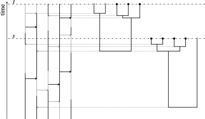
Figure 1: Graphical construction of a tree-valued Moran model with two types with mutation and selection. The fitter type is drawn by the black line and the weaker type by the gray line. In the left part of the figure the gray arrows are used independently of color of the involved lines whereas the black arrows are only used if they start from a black line. Changes of color along a single line are due to mutations. The right part shows how the percolation structure on $S_{N}$ gives rise to a genealogical tree, that is, a (pseudo-)metric space on the set of leaves. The leaves of the tree are marked by the types of the corresponding individuals.

The starting point of our investigation is the continuous-time Moran model with mutation and selection. This is a model of a population of finitely many (distinct) individuals evolving under resampling, mutation and selection and is best studied by its graphical representation. At any fixed time, this representation generates a genealogical tree marked with types; see also Figure 1. In a straightforward way, this allows us to introduce dynamics of genealogies with marks (types) as piecewise deterministic Markov process with jumps. We show that the large population limit of this collection of tree-valued Markov processes exists and is the unique solution of a martingale problem (Theorems 1 and 3). The resulting process is an enrichment of the measure-valued process and we call it the tree-valued Fleming–Viot process with mutation and selection (TFVMS). On the way, we develop the stochastic analysis for tree-valued processes. In particular, we give a Girsanov-transform for our processes and show that genealogies with and without selection can be studied using a change of measure (Theorem 2).

We continue by showing that the function-valued dual for the Fleming–Viot process [see, e.g., Dawson (1993)] works in the tree-valued setting. Using this duality and ideas from Dawson and Greven (2011, 2012a, 2012b), we obtain a stochastic representation for the expectation of functionals of sampled finite marked subtrees. As an application we establish the long-time behavior and the ergodicity of the TFVMS (Theorem 4), if the measure-valued Fleming–Viot process is ergodic. We use this equilibrium to study an important quantity in empirical population genetics in the case of two allelic types and additive selection: the genealogical distance of two randomly sampled individuals of the population. We compute the Laplace transform of the genealogical distance of two sampled individuals in the case where the selection coefficient is small (Theorem 5). This result suggests that tree-lengths are shorter under additive selection. This assertion is widely believed to be true among biologists, but has never been proved.

Our construction gives a process on the space of marked trees, which we can treat as marked metric measure spaces. For convenience, we choose the space of types to be a compact metric space. For the construction, we require knowledge of fundamental topological properties of the marked metric measure spaces. While the case without marks is treated in Greven, Pfaffelhuber and Winter (2009), topological properties for the case with marks are developed in Depperschmidt, Greven and Pfaffelhuber (2011).

2 Moran models with mutation and selection

In this section, we first describe a version of the Moran model with mutation and selection (Section 2.1), its graphical construction (Section 2.2) and then extend the description to the tree-valued case (Section 2.3). Finally, we discuss various aspects of models including selection (Section 2.4).

2.1 The dynamics of the Moran model

Fix $N\in\mathbb{N}$, the population size of the Moran model. Every individual carries an (allelic) type, element of a set $I$, and we assume that

$$I\mbox{ is a compact metric space}$$ (1)

for convenience. The individuals of the population are denoted by $k,l,\ldots\in\{1,\ldots,N\}$. The initial configuration is $(u_{1}(0),\ldots,u_{N}(0))$, where $u_{k}(0)\in I$ denotes the initial type of individual $k$. The population evolves as a pure jump Markov process, and the dynamics are given through the following mechanisms.

[$\blacktriangleright$]

Resampling (also known as pure genetic drift): every (unordered) pair $k\neq l$ is replaced at the resampling rate

$$\gamma>0.$$ (2)

Upon such a resampling event, $l$ is replaced by an offspring of $k$, or $k$ is replaced by an offspring of $l$, each with probability $\frac{1}{2}$. In other words, for every ordered pair $k\neq l$, individual $l$ is replaced by an offspring of $k$ at rate $\frac{\gamma}{2}$.

Mutation: the type of every individual changes from $u$ to $v$ at rate

$$\vartheta\cdot\beta(u,dv),$$ (3)

where $\vartheta\geq 0$ (the mutation rate) and $\beta(\cdot,\cdot)$ is a stochastic kernel on $I$. For selection, we have two different cases. (See also the discussion in Section 2.4 on other forms of selection.) Individuals are either haploid or diploid.

[$\blacktriangleright$]

Haploid selection: every (ordered) pair $k\neq l$ is involved in a selection event at rate

$$\frac{\alpha}{N}\cdot\chi(u_{k})$$ (4)

for $\alpha\geq 0$ (the selection coefficient) and measurable fitness function $\chi\dvtx I\to[0,1]$. Upon a selective event, individual $l$ is replaced by an offspring of individual $k$.

Diploid selection: every (ordered) triple of pairwise distinct $k,l,m$ is involved in a selection event at rate

$$\frac{\alpha}{N^{2}}\cdot\chi^{\prime}(u_{k},u_{m})$$ (5)

for $\alpha\geq 0$ and a symmetric $[0,1]$-valued function $\chi^{\prime}$ with $\chi^{\prime}(u,v)=\chi^{\prime}(v,u)$, which denotes the fitness of the diploid $\{u,v\}$. Again, individual $l$ is replaced by an offspring of individual $k$.

Remark 2.1 ((Diploid selection)).

While the mechanism for haploid selection is intuitively clear, the diploid case requires some explanation. Here, $N$ is the number of haploid individuals, which are arranged in pairs to form diploids. Since the formation of diploids according to the type frequencies of the haploids acts on a fast timescale, we can assume that the population is in Hardy–Weinberg equilibrium at all times, meaning that the diploid individuals are random pairs of haploids, and this formation is independent for all times.

Actually, to model diploid selection, we would have to say that every quadruple $k,l,m,n$ of pairwise distinct individuals is involved in a selective event at rate $\alpha\cdot\chi^{\prime}(u_{k},u_{m})/N^{3}$ in which the haploid $l$ from the diploid individual $\{l,n\}$ is replaced by an offspring of haploid $k$ from the diploid individual $\{k,m\}$. However, as the haploid individual $n$ is not affected by such events, our definition above is appropriate.

Haploid and diploid selection leads to the same dynamics in special cases. In the large population limit, we see that diploid selection reduces to the haploid case for additive fitness, that is, if $\chi^{\prime}$ is of the form $\chi^{\prime}(u,v)=\chi(u)+\chi(v)$ for some function $\chi$; see (34) and (37).

2.2 The graphical construction

A useful construction of the Moran model is by means of a random graph whose main benefit is to automatically generate ancestral lines explicitly. For instance, we use these ancestral lines in order to bound the number of ancestors of the whole population (Proposition 6.9) and show tightness of a sequence of tree-valued Moran models (see the proof of Theorem 3).

Definition 2.2 ((Graphical construction of the Moran model)).

For fixed $N\in\mathbb{N}$, set

$$U_{N}=\{1,\ldots,N\},$$

and consider the following families of independent Poisson point processes:

$$\eta_{\mathrm{res}} := \{\eta_{\mathrm{res}}^{k,l}\dvtx k,l\in U_{N}\}\qquad\mbox{each $\eta_{\mathrm{res}}^{k,l}$ with rate }\frac{\gamma}{2},$$

$$\eta_{\mathrm{mut}} := \{\eta_{\mathrm{mut}}^{k}\dvtx k\in U_{N}\}\qquad\mbox{each $\eta_{\mathrm{mut}}^{k}$ with rate }\vartheta$$

and

$$\mbox{haploid selection: }\eta_{\mathrm{sel}} := \{\eta_{\mathrm{sel}}^{k,l}\dvtx k,l\in U_{N}\}\qquad\mbox{each $\eta_{\mathrm{sel}}^{k,l}$ with rate }\frac{\alpha}{N},$$

$$\mbox{diploid selection: }\eta_{\mathrm{sel}} := \{\eta_{\mathrm{sel}}^{k,l,m}\dvtx k,l,m\in U_{N}\}\qquad\mbox{each $\eta_{\mathrm{sel}}^{k,l,m}$ with rate }\frac{\alpha}{N^{2}}.$$

The graphical construction of the particle system defines a percolation structure on the set $S_{N}:=U_{N}\times[0,\infty)$. If $t\in\eta_{\mathrm{res}}^{k,l}$, we draw an arrow from $(k,t)$ to $(l,t)$. If $t\in\eta_{\mathrm{sel}}^{k,l}$ in the haploid case, or $t\in\eta_{\mathrm{sel}}^{k,l,m}$ in the diploid case, draw a selective arrow from $(k,t)$ to $(l,t)$ in the haploid case and two different selective arrows from $(k,t)$ to $(l,t)$ and from $(m,t)$ to $(l,t)$.

Finally, consider the type process $(u_{k}(t))_{k\in U_{N},t\geq 0}$, starting in $u_{1}(0),\ldots,\break u_{N}(0)$. Upon a resampling event $t\in\eta_{\mathrm{res}}^{k,l}$, set $u_{l}(t)=u_{k}(t-)$. In addition, we say that $(k,t-)$ is the ancestor of $(l,t)$ at time $t-$. For $t\in\eta_{\mathrm{sel}}^{k,l}$, a selective event takes place with probability $\chi(u_{k}(t-))$ in the haploid case. In this case we set $u_{l}(t)=u_{k}(t-)$ and say that $(k,t-)$ is the ancestor of $(l,t)$ at time $t-$. In the diploid case a selective event $t\in\eta_{\mathrm{sel}}^{k,l,m}$ takes place with probability $\chi^{\prime}(u_{k}(t-),u_{m}(t-))$, and we set $u_{l}(t)=u_{k}(t-)$. In this case $(k,t-)$ is ancestor of $(l,t)$ at time $t-$. Mutation events take place at times $t\in\eta_{\mathrm{mut}}^{k}$ where we set $u_{k}(t)=v$ with probability $\beta(u_{k}(t-),dv)$.

Example 2.3 ((Example with haploid selection and two types)).

The left part of Figure 1 illustrates the graphical construction of the Moran model in the special case $N=5$, haploid selection, $I=\{\bullet,{\mbox{ \includegraphics{831i01.eps} }}\}$ and $\chi=\mathbh{1}_{\{\bullet\}}$; that is, $\bullet$ is fit and is unfit. Mutation from to $\bullet$ and vice versa occurs at two possibly different rates, denoted $\vartheta_{\mbox{ \includegraphics{831i02.eps} }}$ and $\vartheta_{\bullet}$. Resampling arrows in $\eta_{\mathrm{res}}$ are drawn in gray, while selective arrows in $\eta_{\mathrm{sel}}$ are black. Thus, the gray arrows are always used, whereas the black arrows are only used if they start from black lines.

Remark 2.4 ((Convergence to the Fleming–Viot process)).

Consider the graphical construction of a Moran model of size $N$ with mutation and selection from Definition 2.2. For any $t$, the types $u_{1}(t),\ldots,u_{N}(t)\in I$ of individuals $1,\ldots,N$ at time $t$ can be read off. We define the $N$th empirical type distribution process $\zeta^{N}=(\zeta^{N}_{t})_{t\geq 0}$ by

$$\zeta^{N}_{t}:=\frac{1}{N}\sum_{k=1}^{N}\delta_{u_{k}(t)}.$$ (6)

It is well known that $\zeta^{N}\stackrel{{\scriptstyle N\to\infty}}{{\Longrightarrow}}\zeta$, where $\zeta=(\zeta_{t})_{t\geq 0}$ is the measure-valued Fleming–Viot process with mutation and selection; see, for example, Dawson (1993), Ethier and Kurtz (1993), Etheridge (2001). In Example 3.9, we recall its definition via a martingale problem.

2.3 The tree-valued Moran model

We are now prepared to define the tree-valued stochastic process arising from the Moran model with mutation and selection, in terms of the graphical construction from Definition 2.2. For this purpose we will need the notion of ancestors. From Figure 1 it is clear that every $l\in U_{N}$ at time $t$ has an ancestor $A_{s}(l,t)\in U_{N}$ at time $s<t$.

Definition 2.5 ((Tree-valued Moran model with mutation and selection)).

We use the same notation as in Definition 2.2. For every $(l,t)\in S_{N}$, define the $U_{N}$-valued, piecewise constant process $(A_{s}(l,t))_{0\leq s\leq t}$ that jumps from $k$ at time $s$ to $j$ at time $s-$, if $(j,s-)$ is an ancestor of $(k,s)$ at time $s-$. We then say that $A_{s}(l,t)$ is the ancestor of $(l,t)$ at time $s$.

The tree-valued Moran model of size $N$ with mutation and selection takes values in triples $(U_{N},r^{N},\mu^{N})$, where $r^{N}$ is a pseudo-metric on $U_{N}$ [i.e., $r^{N}(k,l)=0$ is allowed for $k\neq l$] and $\mu^{N}$ is a probability measure on $U_{N}\times I$.

Starting in a pseudo-metric $r_{0}^{N}$ on $U_{N}$, we define for $k,l\in U_{N}$ and $t\geq 0$

$$\quad r^{N}_{t}(k,l):=\cases{2\bigl{(}t-\sup\{s\dvtx A_{s}(k,t)=A_{s}(l,t)\}\bigr{)},\vspace*{2pt}\cr\hskip 122.7pt\qquad\mbox{if $A_{0}(k,t)=A_{0}(l,t)$},\vspace*{2pt}\cr 2t+r_{0}^{N}(A_{0}(k,t),A_{0}(l,t)),\qquad\mbox{else},}$$

a pseudo-metric $r^{N}_{t}$ on $U_{N}$, such that $r^{N}_{t}(k,l)$ is twice the time to the most recent common ancestor of $k$ and $l$. Finally, we define the sampling measure as

$$\mu^{N}_{t}:=\frac{1}{N}\sum_{k=1}^{N}\delta_{(k,u_{k}(t))}.$$ (7)

Then the tree-valued Moran model with mutation and selection is given by

$$((U_{N},r^{N}_{t},\mu^{N}_{t}))_{t\geq 0}.$$ (8)

Example 2.6 ((Example with two types)).

Let us again consider Example 2.3 and Figure 1. For any time $t$, a genealogical tree can be read off for the individuals $(1,t),\ldots,(5,t)$, giving rise to a (pseudo-)metric on $U_{5}$ based on genealogical distances. In addition, the types $u_{1}(t),\ldots,u_{5}(t)$ are encoded in the graphical representation as well and give rise to the empirical measure $\zeta_{t}^{5}$.

Remark 2.7 ((Trees as marked metric measure spaces, mark functions)).

(1) Recall that an ultrametric space can be mapped isometrically in a unique way onto the set of leaves of a rooted $\mathbb{R}$-tree, justifying the name tree-valued; see also Remark 2.2 in Greven, Pfaffelhuber and Winter (2012).

(2) We call the states $(U_{N},r^{N}_{t},\mu^{N}_{t})$ marked metric measure spaces (or mmm-spaces); see also Definition 3.2. To define an appropriate notion of convergence, we will have to pass from $(U_{N},r^{N}_{t},\mu^{N}_{t})$ to equivalence classes (also defined in detail in Definition 3.2). Roughly speaking, $(U_{N},r^{N},\mu^{N})$ and $(U_{N},{r^{\prime}}^{N},{\mu^{\prime}}^{N})$ are equivalent, if there is a bijection $\sigma$ on $U_{N}$ with $r^{N}(\sigma(i),\sigma(j))={r^{\prime}}^{N}(i,j)$, and ${\mu^{\prime}}^{N}$ is the image of $\mu^{N}$ under the reordering $\sigma$. We will write

$$\mathcal{U}^{N}_{t}=\overline{(U_{N},r^{N}_{t},\mu^{N}_{t})}$$ (9)

for the equivalence class of $(U_{N},r^{N}_{t},\mu^{N}_{t})$, and call $\mathcal{U}^{N}=(\mathcal{U}_{t}^{N})_{t\geq 0}$ the tree-valued Moran model with mutation and selection (TMMMS).

(3) For the tree-valued Moran model, $((U_{N},r_{t}^{N},\mu^{N}_{t}))_{t\geq 0}$, we can define a mark function, $\kappa_{t}(k):=u_{k}(t)$. Moreover, resampling/selection and mutation occur at different time points, which implies that $\kappa_{t}$ is measurable with respect to the Borel-$\sigma$-algebra of $(U_{N},r^{N}_{t})$ for all $t\geq 0$, almost surely. In particular, $\mu^{N}_{t}$ has the special form

$$\mu^{N}_{t}(dx,du)=\Biggl{(}\frac{1}{N}\sum_{k=1}^{N}\delta_{k}(dx)\Biggr{)}\cdot\delta_{\kappa_{t}(x)}(du).$$ (10)

See Remark 3.11 for more on mark functions in the large population limit.

2.4 Background on selection

Since fitness is the fundamental concept in Darwin’s Origin of Species, selection is the most important feature of population models in biology. A vast amount of literature is devoted to this topic. We briefly discuss aspects related to the tree-valued processes.

Fertility, viability and state-dependent selection

In a selective event of the Moran model described in Section 2.1, an individual replaces a randomly drawn individual, independent of the fitness of the replaced individual. Thus, we take the special form of fertility selection here; that is, individuals might have a fitness bonus which determines their chances to produce a higher number of offspring. Sometimes, this is also called positive selection.

In the case of viability or negative selection, individuals have a fitness malus, which determines their chances to die and be replaced by the offspring of a randomly drawn individual. In the case of viability selection acting on haploids, we would have a fitness function $\widetilde{\chi}\dvtx I\to[0,1]$, and every ordered pair $k\neq l$ is involved in a selective event at rate $\alpha\cdot\widetilde{\chi}(u_{l})/N$. Upon such an event, individual $l$ is replaced by an offspring of individual $k$. Our main results, Theorems 1–5, carry over to the situation of viability selection.

Also the state-dependent selection can be incorporated in our model. For this, recall the empirical type distribution $\zeta^{N}$ of the Moran model of size $N$ from Remark 2.4. Consider the fitness function $\chi^{\prime\prime}\dvtx I\times\mathcal{M}_{1}(I)\to[0,1]$, that is, $\chi^{\prime\prime}(u,\zeta)$ is the fitness of type $u$ if the type distribution of the total population is $\zeta$. An offspring of individual $k$ replaces the individual $l$ at rate $\frac{\alpha}{N}\cdot\chi^{\prime\prime}(u_{k},\zeta)$. However, if

$$\chi^{\prime\prime}(u,\zeta)=\int\chi^{\prime}(u,v)\zeta(dv)$$ (11)

for some $\chi^{\prime}\dvtx I\times I\to[0,1]$ we find that an offspring of individual $k$ replaces individual $l$ at selective events occurring at rate

$$\frac{\alpha}{N}\cdot\chi^{\prime\prime}(u_{k},\zeta)=\frac{\alpha}{N}\cdot\int\chi^{\prime}(u_{k},v)\zeta(dv)=\frac{\alpha}{N^{2}}\sum_{m=1}^{N}\chi^{\prime}(u_{k},u_{m}).$$ (12)

So, if (11) holds, (5) shows that state-dependent selection is the same as diploid selection. Compare also Section 7.6 in Etheridge (2001).

Kin selection

For measure-valued processes, selection is modeled by a symmetric function $\widehat{\chi}^{\prime}\dvtx I\times I\to\mathbb{R}$; see Definition 2.2. In the TMMMS we encode both, the type distribution and the genealogical tree in the process. This allows us to treat diploid selection depending also on genealogical distance; that is, we can deal with fitness functions of the form

$$\chi\dvtx I\times I\times\mathbb{R}_{+}\longrightarrow[0,1].$$ (13)

Here, $\chi(u,v,r)$ is the fitness of a diploid individual with genotype $\{u,v\}$ if the genealogical distance of the two haploids forming the diploid individual is $r$. Equivalently, if $\mathpzc{u}=\overline{(U_{N},r^{N},\mu^{N})}$ is the current state of the TMMMS, then the offspring of the haploid individual $k\in U_{N}$ replaces individual $l\in U_{N}$ at a selective event taking place at rate

$$\frac{\alpha}{N}\cdot\sum_{m=1}^{N}\chi(u_{k},u_{m},r^{N}(k,m)).$$ (14)

A special case of selection depending on genealogical distance is kin selection [e.g., Uyenoyama, Feldman and Mueller (1981)], leading to the concept of inclusive fitness [Hamilton (1964a, 1964b)]. The idea is that the fitness of an individual is higher if close relatives are around who can help to raise offspring. Such an altruistic behavior can evolve since it might also be beneficial for the helpers, because offspring of close relatives is likely to carry similar genetic material. Such a scenario can be modeled using a fitness function of the form (14) that is decreasing in its third coordinate, that is, in the genealogical distance.

The ancestral selection graph of Krone and Neuhauser

Genealogies under selection were studied in Neuhauser and Krone (1997) and Krone and Neuhauser (1997) by introducing the ancestral selection graph (ASG). The construction can easily be explained using Figure 1. Suppose that we are interested in the genealogy at time $t$. The ASG produces the genealogy in a three-step procedure from present to the past. Most importantly, when working backward in time, it is not known in advance if a selective arrow is used or not. [(2)]

Going from the top downward through the graphical representation, consider first the resampling and selective arrows. Two lines coalesce when a resampling event occurs between them. If a line hits the tip of a selective arrow, a branching event occurs. One line, the continuing line, is followed in order to get information on the ancestral line if the selective arrow is not used, and the other line, the incoming line, is followed if the selective arrow is used. Wait until time 0 and stop the process.

At time $0$, mark all individuals according to the initial distribution, and superimpose the mutation process along the graph, from time $0$ to time $t$.

Go through all selective arrows between times $0$ and $t$. Follow the continuing line if the arrow does not go from a black line to a gray line, because in this case, the selection event is not realized. In the other cases, take the incoming branch. As a result, one obtains genealogical distances of the time $t$ population, together with their types. The main difference between the ASG and our construction is that the ASG gives the genealogy only at a single time, while we describe evolving genealogies. However, our dual process in Section 5 is reminiscent of the ASG.

Outline: The paper is organized as follows. In Section 3, we state our main results on the TFVMS process. In Sections 4 and 5 we develop some tools which are not only needed in the proofs of the main results, but are also of interest in their own right. The techniques we use are a detailed analysis of the generator of TFVMS (Section 4) and duality of Markov processes (Section 5). In Section 6 we state and prove important facts concerning the Moran model. For instance, we give the generator characterization of the finite population model (TMMMS) and discuss properties of numbers of ancestors and descendants. Finally, the proofs of our main results are given in Sections 7 and 8.

We collect the most important notation needed in the paper in the Appendix.

3 Results

In this section we formulate our main results in the set-up of and under assumptions listed in Sections 2.1 and 2.3. Our main point is to establish that the weak limit of the process $((U_{N},r^{N}_{t},\mu^{N}_{t}))_{t\geq 0}$ from Definition 2.5 as $N\to\infty$ exists, characterize it intrinsically and to study its properties. The result is the generalization of the convergence of the measure-valued Moran models to the Fleming–Viot diffusion (see Remark 2.4) to the level of marked genealogical trees.

Before we formulate the results, we have to specify the state space and give a summary of its properties in Section 3.1. Afterward, in Section 3.2, we give in Theorem 1 the construction of the TFVMS via a well-posed martingale problem. Theorem 2 in Section 3.3 gives a Girsanov transformation between the neutral and the selective tree-valued processes, and Theorem 3 from Section 3.4 shows that the TFVMS arises as weak limit of TMMMS. The long-time behavior of TFVMS is studied in Theorem 4 of Section 3.5. Finally, an application to genealogical distances of sampled individuals in equilibrium is considered in Section 3.6, in Theorem 5.

Remark 3.1 ((Notation)).

For product spaces $X\times Y\times\cdots,$ we denote by $\pi_{X},\pi_{Y},\ldots$ the projection operators. For a Polish space $E$, the function spaces $\mathcal{B}(E)$ and $\overline{\mathcal{C}}(E)$ denote the bounded measurable and bounded continuous, real-valued functions on $E$, respectively. We denote by $\mathcal{M}_{1}(E)$ the space of probability measures on (the Borel sets of) $E$, equipped with the topology of weak convergence, abbreviated by $\Rightarrow$. For $\mu\in\mathcal{M}_{1}(E)$ and $\phi\in\mathcal{B}(E)$, we set $\langle\mu,\phi\rangle:=\int\phi(x)\mu(dx)$. Moreover, for $\varphi\dvtx E\to E^{\prime}$ (for some other Polish space $E^{\prime}$), the image measure of $\mu$ under $\varphi$ is denoted by $\varphi_{\ast}\mu$. For $A\subseteq\mathbb{R}$, equipped with the Euclidean topology, we denote by $\mathcal{C}_{E}(A)$ ($\mathcal{D}_{E}(A)$) the set of continuous (càdlàg) functions $A\to E$, equipped with the topology of uniform convergence on compact sets (the Skorohod topology).

3.1 State space

Here we introduce the set of isometry classes of marked ultrametric measure spaces (denoted by $\mathbb{U}^{I}$) that will be the state space of both, the TMMMS and the TFVMS. The starting point of our definition are results from Greven, Pfaffelhuber and Winter (2009) that are extended in Depperschmidt, Greven and Pfaffelhuber (2011). While $I$ is a compact metric space in all applications, the notions introduced in this subsection are valid for any Polish space $I$.

Definition 3.2 ((mmm-spaces)).

(1) An $I$-marked metric measure space, $I$-mmm-space or mmm-space, for short, is a triple $(X,r,\mu)$ such that $(X,r)$ is a complete and separable metric space and $\mu\in\mathcal{M}_{1}(X\times I)$. Without loss of generality we assume that $X\subseteq\mathbb{R}$.

(2) An mmm-space $(X,r,\mu)$ is called compact if $(\operatorname{supp}((\pi_{X})_{\ast}\mu),r)$ is compact. It is called ultrametric if $(\operatorname{supp}((\pi_{X})_{\ast}\mu),r)$ is ultrametric.

(3) Two mmm-spaces $(X,r_{X},\mu_{X})$ and $(Y,r_{Y},\mu_{Y})$ are measure-preserving isometric and $I$-preserving (or equivalent), if there exists a measurable map $\varphi\dvtx X\to Y$ such that $r_{X}(x,x^{\prime})=r_{Y}(\varphi(x),\varphi(x^{\prime}))$ for all $x,x^{\prime}\in\operatorname{supp}((\pi_{X})_{\ast}\mu_{X})$ and $\widetilde{\varphi}_{\ast}\mu_{X}=\mu_{Y}$ for $\widetilde{\varphi}(x,u)=(\varphi(x),u)$. The equivalence class of an mmm-space $(X,r,\mu)$ is denoted by $\overline{(X,r,\mu)}$.

(4) We define

$$\mathbb{M}^{I}:=\{\overline{(X,r,\mu)}\dvtx(X,r,\mu)\mbox{ mmm-space}\}.$$ (15)

Moreover,

$$\mathbb{M}^{I}_{c} := \{\overline{(X,r,\mu)}\dvtx(X,r,\mu)\mbox{ compact mmm-space}\},$$

$$\mathbb{U}^{I} := \{\overline{(X,r,\mu)}\dvtx(X,r,\mu)\mbox{ ultrametric mmm-space}\},$$ (16)

$$\mathbb{U}^{I}_{c} := \mathbb{M}^{I}_{c}\cap\mathbb{U}^{I}.$$

Generic elements of $\mathbb{M}^{I}$ ($\mathbb{U}^{I}$) are denoted by $\mathpzc{x},\mathpzc{y},\ldots(\mathpzc{u},\ldots)$.

Remark 3.3 ((Pseudo-metrics)).

Occasionally, we will encounter pseudo-metric spaces $(X,r)$ [i.e., $r(x_{1},x_{2})=0$ for $x_{1}\neq x_{2}$ is possible]. The notion of the equivalence class from Definition 3.2 carries over to marked pseudo-metric measure spaces. Moreover, in the equivalence class $\overline{(X,r,\mu)}$ of a marked pseudo-metric measure space $(X,r,\mu)$, we always find an mmm-space $(X^{\prime},r^{\prime},\mu^{\prime})$, such that the topology on $X$ generated by $r$ is in 1–1 correspondence to the topology on $X^{\prime}$ generated by $r^{\prime}$. That is, the open subsets of $X$ can be mapped onto the open subsets of $X^{\prime}$ and vice versa. In particular, it is no restriction to use marked metric measure spaces instead of marked pseudo-metric measure spaces.

In order to define an appropriate topology on $\mathbb{M}^{I}$, we introduce the notion of the marked distance matrix distribution.

Definition 3.4 ((Marked distance matrix distribution)).

Let $(X,r,\mu)$ be an mmm-space, $\mathpzc{x}:=\overline{(X,r,\mu)}\in\mathbb{M}^{I}$ and

$$R^{(X,r)}\dvtx\cases{(X\times I)^{\mathbb{N}}\to\mathbb{R}_{+}^{{\mathbb{N}\choose 2}}\times I^{\mathbb{N}},\cr((x_{i},u_{i})_{i\geq 1})\mapsto((r(x_{i},x_{j}))_{1\leq i<j},(u_{k})_{k\geq 1}).}$$ (17)

The marked distance matrix distribution of $\mathpzc{x}=\overline{(X,r,\mu)}$ is given by

$$\nu^{\mathpzc{x}}:=\bigl{(}R^{(X,r)}\bigr{)}_{\ast}\mu^{\mathbb{N}}\in\mathcal{M}_{1}\bigl{(}\mathbb{R}^{{\mathbb{N}\choose 2}}\times I^{\mathbb{N}}\bigr{)}.$$ (18)

Remark 3.5 ((Distance matrix distribution is exchangeable)).

(1) Note that $(R^{(X,r)})_{\ast}\mu^{\mathbb{N}}$ in the above definition does not depend on the particular element $(X,r,\mu)$ of $\mathpzc{x}=\overline{(X,r,\mu)}$. In particular, $\nu{x}$ is well defined. Moreover, by Theorem 1 in Depperschmidt, Greven and Pfaffelhuber (2011), we have $\mathpzc{x}=\mathpzc{y}$ if and only if $\nu{x}=\nu{y}$.

(2) Let

$$\Sigma:=\{\sigma\dvtx\mathbb{N}\to\mathbb{N}|\mbox{$\sigma$ is injective}\}$$ (19)

be the set of injective maps on $\mathbb{N}$. For $\sigma\in\Sigma$, set

$$R_{\sigma}\dvtx\cases{\mathbb{R}_{+}^{{\mathbb{N}\choose 2}}\times I^{\mathbb{N}}\to\mathbb{R}_{+}^{{\mathbb{N}\choose 2}}\times I^{\mathbb{N}},\vspace*{2pt}\cr((r_{ij})_{1\leq i<j},(u_{k})_{k\geq 1})\mapsto\bigl{(}\bigl{(}r_{\sigma(i)\wedge\sigma(j),\sigma(i)\vee\sigma(j)}\bigr{)},\bigl{(}u_{\sigma(k)}\bigr{)}_{k\geq 1}\bigr{)}.}$$ (20)

Then, for $\mathpzc{x}\in\mathbb{M}^{I}$, the measure $\nu{x}$ is exchangeable in the sense that

$$(R_{\sigma})_{\ast}\nu{x}=\nu{x}.$$ (21)

Definition 3.6 ((Marked Gromov-weak topology)).

Let $\mathpzc{x},\mathpzc{x}_{1},\mathpzc{x}_{2},\ldots\in\mathbb{M}^{I}$. We say that $\mathpzc{x}_{n}\to\mathpzc{x}$ as $n\to\infty$ in the marked Gromov-weak topology if

$$\nu^{\mathpzc{x}_{n}}\stackrel{{\scriptstyle n\to\infty}}{{\Longrightarrow}}\nu{x}$$ (22)

in the weak topology on $\mathcal{M}_{1}(\mathbb{R}_{+}^{{\mathbb{N}\choose 2}}\times I^{\mathbb{N}})$, where, as usual, ${\mathbb{R}}_{+}^{{\mathbb{N}\choose 2}}\times I^{\mathbb{N}}$ is equipped with the product topology of ${\mathbb{R}}_{+}$ and $I$, respectively.

Several topological facts on the marked Gromov-weak topology were established in Depperschmidt, Greven and Pfaffelhuber (2011). One of the most important, showing that $\mathbb{M}^{I}$ is a space suitable for probability theory, is that the space $\mathbb{M}^{I}$ is Polish [Theorem 2 in Depperschmidt, Greven and Pfaffelhuber (2011)]. Before we state our results, we need to introduce several function spaces on $\mathbb{M}^{I}$.

Definition 3.7 ((Polynomials)).

(1) We denote by

$$\mathcal{B}_{n} := \mathcal{B}_{n}\bigl{(}\mathbb{R}_{+}^{{\mathbb{N}\choose 2}}\times I^{\mathbb{N}}\bigr{)},\qquad\overline{\mathcal{C}}_{n}:=\overline{\mathcal{C}}_{n}\bigl{(}\mathbb{R}_{+}^{{\mathbb{N}\choose 2}}\times I^{\mathbb{N}}\bigr{)},$$

$$\overline{\mathcal{C}}{}^{1}_{n} := \overline{\mathcal{C}}{}^{1}_{n}\bigl{(}\mathbb{R}_{+}^{{\mathbb{N}\choose 2}}\times I^{\mathbb{N}}\bigr{)},$$

the sets of bounded measurable (continuous, continuous and continuously differentiable with respect to all variables in $\mathbb{R}_{+}^{{\mathbb{N}\choose 2}}$) functions $\phi$ on $\mathbb{R}_{+}^{{\mathbb{N}\choose 2}}\times I^{\mathbb{N}}$, such that $(\underline{\underline{r}},\underline{u})\mapsto\phi(\underline{\underline{r}},\underline{u})$ depends on the first ${n\choose 2}$ variables in $\underline{\underline{r}}$ and the first $n$ in $\underline{u}$ only. (If $n=0$, the spaces consist of constant functions.)

(2) A function $\Phi\dvtx\mathbb{M}^{I}\to\mathbb{R}$ is a polynomial if, for some $n\in\mathbb{N}$, there exists $\phi\in\mathcal{B}_{n}$, such that for all $\mathpzc{x}\in\mathbb{M}^{I}$,

$$\Phi(\mathpzc{x}):=\Phi^{n,\phi}=\langle\nu{x},\phi\rangle=\int\phi(\underline{\underline{r}},\underline{u})\nu{x}(d\underline{\underline{r}},d\underline{u}).$$ (24)

(3) The degree of a polynomial $\Phi$ is the smallest number $n$ for which there exists $\phi\in\mathcal{B}_{n}$ such that (24) holds.

(4) Writing $\overline{\mathcal{C}}{}^{0}_{n}:=\overline{\mathcal{C}}_{n}$, we set

$$\Pi := \bigcup_{n=0}^{\infty}\Pi_{n},\qquad\Pi_{n}:=\{\Phi^{n,\phi}\dvtx\phi\in\mathcal{B}_{n}\},$$

$$\Pi^{k} := \bigcup_{n=0}^{\infty}\Pi^{k}_{n},\qquad\Pi_{n}^{k}:=\{\Phi^{n,\phi}\dvtx\phi\in\overline{\mathcal{C}}{}^{k}_{n}\},\qquad k=0,1.$$

We use the sets of polynomials as domains for the generator of the TFVMS process. In this context, we require that $\Pi^{1}$ is an algebra that separates points, a result proved in Proposition 4.1 in Depperschmidt, Greven and Pfaffelhuber (2011).

3.2 Martingale problem

In this subsection, we define the TFVMS dynamics by a well-posed martingale problem. First we recall the notion of martingale problems that we use here; see Ethier and Kurtz (1986). Throughout the following, $I$ is assumed to be a compact metric space (and hence Polish).

Definition 3.8 ((Martingale problem)).

Let $E$ be a Polish space, $\mathbf{P}_{0}\in\mathcal{M}_{1}(E)$, $\mathcal{F}\subseteq{\mathcal{B}}(E)$ and $\Omega$ a linear operator on ${\mathcal{B}}(E)$ with domain $\mathcal{F}$. The law $\mathbf{P}$ of an $E$-valued stochastic process $\mathcal{X}=(X_{t})_{t\geq 0}$ is called a solution of the $(\mathbf{P}_{0},\Omega,\mathcal{F})$-martingale problem if $X_{0}$ has distribution $\mathbf{P}_{0}$, $\mathcal{X}$ has paths in the space ${\mathcal{D}}_{E}([0,\infty))$, almost surely, and for all $F\in\mathcal{F}$,

$$\biggl{(}F(X_{t})-\int_{0}^{t}\Omega F(X_{s})\,ds\biggr{)}_{t\geq 0}$$ (26)

is a $\mathbf{P}$-martingale with respect to the canonical filtration. Moreover, the $(\mathbf{P}_{0},\Omega,\mathcal{F})$-martingale problem is said to be well-posed if there is a unique solution $\mathbf{P}$.

As an example we now give the martingale problem characterization of the classical Fleming–Viot diffusion to prepare for the tree-valued process.

Example 3.9 ((The measure-valued Fleming–Viot process)).

We recall the classical Fleming–Viot measure-valued diffusion $\zeta=(\zeta_{t})_{t\geq 0}$ with mutation and selection. It arises as the large population limit of the process describing the evolution of type frequencies $\zeta^{N}=(\zeta^{N}_{t})_{t\geq 0}$ in the Moran models introduced in Section 2. The state space is $\mathcal{M}_{1}(I)$, and $\zeta_{t}$ describes the distribution of allelic types in the population at time $t$.

The process can be characterized in various ways by a martingale problem, for example, by a second order differential operator on $\overline{\mathcal{C}}(\mathcal{M}_{1}(I))$ with domain $\overline{\mathcal{C}}{}^{2}(\mathcal{M}_{1}(I))$, with an appropriate definition of the derivative. However, our choice of an operator on polynomials reveals best the connection to the tree-valued process.

Define the set of polynomials $\mathcal{F}$ on $\mathcal{M}_{1}(I)$ by letting $\mathcal{F}=\bigcup_{n=0}^{\infty}\mathcal{F}_{n}$, where $\mathcal{F}_{n}$ is the set of functions $\widehat{\Phi}\dvtx\mathcal{M}_{1}(I)\to\mathbb{R}$ with $\widehat{\Phi}(\zeta)=\langle\zeta^{\otimes\mathbb{N}},\widehat{\phi}\rangle$ for some $\widehat{\phi}\in\overline{\mathcal{C}}(I^{\mathbb{N}})$, depending only on the first $n$ variables. Define the linear operator on $\overline{\mathcal{C}}(\mathcal{M}_{1}(I))$ with domain $\mathcal{F}$

$$\widehat{\Omega}=\widehat{\Omega}^{\mathrm{res}}+\widehat{\Omega}^{\mathrm{mut}}+\widehat{\Omega}^{\mathrm{sel}}.$$ (27)

Here, for $\widehat{\Phi}\in\mathcal{F}_{n}$ with $\widehat{\Phi}(\zeta)=\langle\zeta^{\otimes\mathbb{N}},\widehat{\phi}\rangle$, the different terms are given as follows: [(2)]

For resampling rate $\gamma>0$, the resampling operator is defined by

$$\widehat{\Omega}^{\mathrm{res}}\widehat{\Phi}(\zeta)=\frac{\gamma}{2}\sum_{k,l=1}^{n}\langle\zeta^{\otimes\mathbb{N}},\widehat{\phi}\circ\widehat{\theta}_{k,l}-\widehat{\phi}\rangle,$$ (28)

where the replacement operator $\widehat{\theta}_{k,l}$ is the map which replaces the $l$th component of an infinite sequence by the $k$th; that is, for $\underline{u}=(u_{1},u_{2},\ldots)$,

$$\widehat{\theta}_{k,l}(\underline{u}) := \underline{u}_{l}^{u_{k}},$$

$$\underline{u}_{l}^{v} := (u_{1},\ldots,u_{l-1},v,u_{l+1},\ldots).$$

For mutation rate $\vartheta\geq 0$, the mutation operator is defined by

$$\widehat{\Omega}^{\mathrm{mut}}\widehat{\Phi}(\zeta)=\vartheta\sum_{k\geq 1}\langle\zeta^{\otimes\mathbb{N}},\widehat{B}_{k}\widehat{\phi}\rangle,$$ (30)

where, for some stochastic kernel $\beta(\cdot,\cdot)$ on $I$,

$$\widehat{B}_{k}\widehat{\phi} := \widehat{\beta}_{k}\widehat{\phi}-\widehat{\phi},$$

$$(\widehat{\beta}_{k}\widehat{\phi})(\underline{u}) := \int\widehat{\phi}(\underline{u}_{k}^{v})\beta(u_{k},dv).$$

That is, $\widehat{B}$ is the bounded generator of a Markov jump process on $I$ with càdlàg paths. It is always possible to write

$$\beta(u,dv)=z\overline{\beta}(dv)+(1-z)\widetilde{\beta}(u,dv)$$ (32)

for some $z\in[0,1]$, $\overline{\beta}\in\mathcal{M}_{1}(I)$ and a stochastic kernel $\widetilde{\beta}(\cdot,\cdot)$ on $I$. We refer to the case $z=1$ as parent-independent mutation or the house-of-cards model. The latter was introduced in Kingman (1978) who argued that mutations might destroy the fragile fitness advantage, which was built up during evolution, and lead to a replacement with an independent type. In this case,

$$\beta(u,dv)=\overline{\beta}(dv)\qquad\mbox{does not depend on }u\in I.$$ (33)

For $z\in(0,1]$, we say that mutation has a parent-independent component.

For selection intensity $\alpha\geq 0$, the selection operator is given by

$$\widehat{\Omega}^{\mathrm{sel}}\widehat{\Phi}(\zeta)=\alpha\sum_{k\geq 1}\langle\zeta^{\otimes\mathbb{N}},\widehat{\phi}\cdot{\widehat{\chi}}^{\prime}_{k,n+1}-\widehat{\phi}\cdot{\widehat{\chi}}^{\prime}_{n+1,n+2}\rangle.$$ (34)

Here, the fitness function

$$\widehat{\chi}^{\prime}\dvtx I\times I\to[0,1]$$ (35)

is measurable and symmetric in both coordinates, and ${\widehat{\chi}^{\prime}}_{k,l}$ acts on the $k$th and $l$th coordinate. The special case for $\chi^{\prime}$, when there exists a function

$$\widehat{\chi}\dvtx I\to[0,1]\qquad\mbox{with }\widehat{\chi}^{\prime}(u,v)=\widehat{\chi}(u)+\widehat{\chi}(v)$$ (36)

is called additive selection or haploid selection. In this case,

$$\widehat{\Omega}^{\mathrm{sel}}\widehat{\Phi}(\zeta)=\alpha\sum_{k\geq 1}\langle\zeta^{\otimes\mathbb{N}},\widehat{\phi}\cdot\widehat{\chi}_{k}-\widehat{\phi}\cdot\widehat{\chi}_{n+1}\rangle,$$ (37)

where $\widehat{\chi}_{k}$ acts on the $k$th coordinate. Note that selective events lead to replacements of individuals similar to resampling events [see also (117) and (118) in the case of Moran models]. However, the replacement operator $\widehat{\theta}_{k,l}$ does not appear in (34) and (37). The reason (in the haploid case) is that the chance that the $k$th individual reproduces through a resampling event depends only on the fitness difference to a randomly chosen individual from the population. See also (6.2), (6.2) and (6.2).

Given $\mathbf{P}_{0}\in\mathcal{M}_{1}(\mathcal{M}_{1}(I))$, it was shown in Ethier and Kurtz (1993) [see also Dawson (1993)] that the $(\mathbf{P}_{0},\widehat{\Omega},\mathcal{F})$-martingale problem is well-posed. We refer to the solution as the (measure-valued) Fleming–Viot process with mutation and selection, FVMS. This is a strong Markov process with continuous paths and hence a diffusion.

More general generators were considered in Dawson and March (1995), where state-dependent resampling and mutation rates were allowed. Selection intensities depending on the state of the FVMS were considered in Donnelly and Kurtz (1999) and unbounded selection operators are studied in Ethier and Shiga (2000). In all these cases well-posedness of the corresponding martingale problem was shown.

Definition 3.10 ((Generator of TFVMS)).

We use the same notation as in Example 3.9. The generator of TFVMS is the linear operator on $\Pi$ with domain $\Pi^{1}$, given by

$$\Omega:=\Omega^{\mathrm{grow}}+\Omega^{\mathrm{res}}+\Omega^{\mathrm{mut}}+\Omega^{\mathrm{sel}}.$$ (38)

Here, for $\Phi^{n,\phi}\in\Pi^{1}_{n}$ the different terms are given as follows: [(2)]

We define the growth operator by

$$\Omega^{\mathrm{grow}}\Phi(\mathpzc{u}):=\langle\nu^{\mathpzc{u}},\langle\nabla_{\underline{\underline{r}}}\phi,\underline{\underline{2}}\rangle\rangle$$ (39)

with

$$\langle\nabla_{\underline{\underline{r}}}\phi,\underline{2}\rangle=2\sum_{1\leq i<j}\frac{\partial\phi}{\partial r_{ij}}(\underline{\underline{r}},\underline{u}).$$ (40)

We define the resampling operator by

$$\Omega^{\mathrm{res}}\Phi(\mathpzc{u}):=\frac{\gamma}{2}\sum_{k,l=1}^{n}\langle\nu{u},\phi\circ\theta_{k,l}-\phi\rangle$$ (41)

with $\theta_{k,l}(\underline{\underline{r}},\underline{u})=(\underline{\underline{\widetilde{r}}},\widehat{\theta}_{k,l}(\underline{u}))$ [recall $\widehat{\theta}_{k,l}$ from (3.9)] and

$$\widetilde{r}_{ij}:=\cases{r_{ij},&\quad if $i,j\neq l$,\cr r_{i\wedge k,i\vee k},&\quad if $j=l$,\cr r_{j\wedge k,j\vee k},&\quad if $i=l$.}$$ (42)

As an example,

$${{\theta_{1,3}(\underline{\underline{r}},\underline{u})=\left(\pmatrix{0&r_{12}&0&r_{14}&r_{15}&\cdots\cr&0&r_{12}&r_{24}&r_{25}&\cdots\cr&&0&r_{14}&r_{15}&\cdots\cr&&&0&r_{45}&\cdots\cr&&&&\cdots&\cdots},(u_{1},u_{2},u_{1},u_{4},u_{5},\ldots)\right).}}$$ (43)

For the mutation operator, let $\vartheta,\beta(\cdot,\cdot)$ be as in Example 3.9, and set

$$\Omega^{\mathrm{mut}}\Phi(\mathpzc{u}):=\vartheta\sum_{k=1}^{n}\langle\nu{u},B_{k}\phi\rangle,$$ (44)

such that

$$B_{k}\phi := \beta_{k}\phi-\phi,$$

$$(\beta_{k}\phi)(\underline{\underline{r}},\underline{u}) := \int\phi(\underline{\underline{r}},\underline{u}_{k}^{v})\beta(u_{k},dv).$$

For selection, consider

$$\chi^{\prime}\dvtx I\times I\times\mathbb{R}_{+}\to[0,1]$$ (46)

with $\chi^{\prime}(u,v,r)=\chi^{\prime}(v,u,r)$ for all $u,v\in I,r\in\mathbb{R}_{+}$; recall (13). In our main results, we require that $\chi^{\prime}\in\overline{\mathcal{C}}{}^{0,0,1}(I\times I\times\mathbb{R}_{+})$; that is, $\chi^{\prime}$ is continuous and continuously differentiable with respect to its third coordinate. Then with

$$\chi^{\prime}_{k,l}(\underline{\underline{r}},\underline{u}):=\chi^{\prime}(u_{k},u_{l},r_{k\wedge l,k\vee l}),$$ (47)

we set

$$\Omega^{\mathrm{sel}}\Phi(\mathpzc{u}):=\alpha\sum_{k=1}^{n}\langle\nu{u},\phi\cdot\chi^{\prime}_{k,n+1}-\phi\cdot\chi^{\prime}_{n+1,n+2}\rangle.$$ (48)

If $\chi^{\prime}(u,v,r)$ does not depend on $r$, and if there is $\chi\dvtx I\to[0,1]$ such that

$$\chi^{\prime}(u,v,r)=\chi(u)+\chi(v)$$ (49)

[compare (36)], we say that selection is additive and conclude that with

$$\chi_{k}(\underline{\underline{r}},\underline{u})=\chi(u_{k}).$$ (50)

We obtain

$$\Omega^{\mathrm{sel}}\Phi(\mathpzc{u}):=\alpha\cdot\sum_{k=1}^{n}\langle\nu{u},\phi\cdot\chi_{k}-\phi\cdot\chi_{n+1}\rangle.$$ (51)

Now, we are ready to give our first main result.

Theorem 1 ((Martingale problem is well posed))

Let $\mathbf{P}_{0}\in\mathcal{M}_{1}(\mathbb{U}^{I})$, $\Pi^{1}$ be as in (3.7) and $\Omega$ as in (38).

1. [(2)]

2. The $(\mathbf{P}_{0},\Omega,\Pi^{1})$-martingale is well posed. The unique solution $\mathcal{U}:=(\mathcal{U}_{t})_{t\geq 0}$ is called the tree-valued Fleming–Viot dynamics with mutation and selection (TFVMS).

3. The process $\mathcal{U}$ has the following properties:

   1. [(a)]

   2. $\mathbf{P}(t\mapsto\mathcal{U}_{t}\mbox{ is continuous})=1$;

   3. $\mathbf{P}(\mathcal{U}_{t}\in\mathbb{U}^{I}_{c}\mbox{ for all }t>0)=1$;

   4. $\mathpzc{u}\mapsto\mathbf{E}[f(\mathcal{U}_{t})|\mathcal{U}_{0}=\mathpzc{u}]$ is continuous for all $f\in\overline{\mathcal{C}}(\mathbb{U}^{I})$, that is, $\mathcal{U}$ has the Feller property;

   5. $\mathcal{U}$ is strong Markov;

   6. for $\Phi=\Phi^{n,\phi}\in\Pi^{1}$, the quadratic variation of the process $\Phi(\mathcal{U})=(\Phi(\mathcal{U}_{t}))_{t\geq 0}$ is given by

      $$[\Phi(\mathcal{U})]_{t}=\gamma\sum_{k,l=1}^{n}\int_{0}^{t}\langle\nu^{\mathcal{U}_{s}},\phi\cdot(\phi\circ\rho_{1}^{n})\cdot\theta_{k,n+l}-\phi\cdot(\phi\circ\rho_{1}^{n})\rangle\,ds,$$ (52)

      where

      $$\rho_{1}^{n}(\underline{\underline{r}},\underline{u})=((r_{i+n,j+n})_{1\leq i<j},(u_{i+n})_{i\geq 1})$$ (53)

      denotes the $n$-shift of the sample sequence.

Remark 3.11 ((Mark function)).

We will show in forthcoming work that states of the TFVMS only take special forms: [(2)]

Consider an mmm-space $\mathpzc{u}=\overline{(U,r,\mu)}\in\mathbb{U}^{I}$. We say that $\mathpzc{u}$ has a mark function if there is an $U$-valued random variable $X$ and $\kappa\dvtx U\to I$ [both measurable with respect to the Borel-$\sigma$-algebra of $(U,r)$] such that $(X,\kappa(X))$ has the distribution $\mu$. In other words, $\mathpzc{u}$ has a mark function if there is a measurable function $\kappa\dvtx U\to I$ with

$$\mu(dx,du)=((\pi_{U})_{\ast}\mu)(dx)\cdot\delta_{\kappa(x)}(du).$$ (54)

As argued in Remark 2.7, the TMMMS always admits states in $\mathbb{U}^{I}$ which have a mark function. It turns out that the same holds for the TFVMS as well.

Another path property we will address are atoms of the measure $\mu$. Consider the TFVMS $\mathcal{U}=(\mathcal{U}_{t})_{t\geq 0}$ with $\mathcal{U}_{t}=\overline{(U,r,\mu)}$. Then, $(\pi_{U})_{\ast}\mu$ has an atom if and only if $\mu^{\otimes 2}\{(x,y)\dvtx r(x,y)=0\}>0$. We shall show that $\mathcal{U}$ only takes values in the space of mmm-spaces $\mathpzc{x}=\overline{(X,r,\mu)}$ with the property that $(\pi_{U})_{\ast}\mu$ has no atoms. Note that only the projection $(\pi_{U})_{\ast}\mu$ can be free of atoms since it is well known that $(\pi_{I})_{\ast}\mu$ is atomic for all $t\geq 0$, almost surely; see, for example, Theorem 10.4.5 in Ethier and Kurtz (1986).

3.3 Girsanov theorem for the TFVMS

One possibility to establish the existence and uniqueness of martingale problems and to analyze its properties is to show that solutions of different martingale problems are absolutely continuous to each other for finite time horizons. Uniqueness as well as several other properties (e.g., path properties) then carry over from one martingale problem to the other. The densities of the solutions of the martingale problems are calculated by the Cameron–Martin–Girsanov theorem for real-valued semimartingales [see Theorem 16.19 in Kallenberg (2002)] and Dawson’s Girsanov theorem for measure-valued processes [Dawson (1993), Section 7.2]. Here, we carry out the corresponding program for TFVMS by considering two martingale problems with different selection strength.

Remark 3.12 ((Notation)).

For $\alpha\in\mathbb{R}_{+}$, we write $\Omega_{\alpha}$ and $\Omega_{\alpha}^{\mathrm{sel}}$ for the operators defined in (38) and (48), respectively, when we want to stress the value of the selection coefficient $\alpha$.

Theorem 2 ((Girsanov Transform for the TFVMS processes))

Let $\alpha,\alpha^{\prime}\in\mathbb{R}_{+}$, $\mathbf{P}_{0}\in\mathcal{M}_{1}(\mathbb{U}^{I})$, and using $\chi^{\prime}_{1,2}$ from (47) define $\Psi\in\Pi^{1}$ by

$$\Psi(\mathpzc{u}):=\frac{\alpha^{\prime}-\alpha}{\gamma}\cdot\langle\nu^{\mathpzc{u}},\chi^{\prime}_{1,2}\rangle.$$ (55)

Let $\mathbf{P}\in\mathcal{M}_{1}(\mathcal{C}_{\mathbb{U}^{I}}(\mathbb{R}_{+}))$ be a solution of the $(\mathbf{P}_{0},\Omega_{\alpha},\Pi^{1})$-martingale problem, $\mathcal{U}=(\mathcal{U}_{t})_{t\geq 0}$ the canonical process with respect to $\mathbf{P}$, $(\mathcal{F}_{t})_{t\geq 0}$ its canonical filtration and

$$\mathcal{M}=(M_{t})_{t\geq 0}=\biggl{(}\Psi(\mathcal{U}_{t})-\Psi(\mathcal{U}_{0})-\int_{0}^{t}\Omega_{\alpha}\Psi(\mathcal{U}_{s})\,ds\biggr{)}_{t\geq 0}.$$ (56)

Then, $\mathcal{M}$ is a $\mathbf{P}$-martingale and the probability measure $\mathbf{Q}$, defined by

$$\frac{d\mathbf{Q}}{d\mathbf{P}}\bigg{|}_{\mathcal{F}_{t}}=e^{M_{t}-(1/2)[\mathcal{M}]_{t}}$$ (57)

solves the $(\mathbf{P}_{0},\Omega_{\alpha^{\prime}},\Pi^{1})$-martingale problem.

3.4 Convergence of Moran models

Our next task is to relate the Fleming–Viot process to the finite population models and their evolving genealogies on the level of trees, that is, mmm-spaces.

Definition 3.13 ((TMMMS)).

Recall the process $(U_{N},r^{N}_{t},\mu^{N}_{t})_{t\geq 0}$ from Definition 2.5, started in a random mmm-space $(U_{N},r^{N}_{0},\mu^{N}_{0})$. The fitness function is either given as in Definition 2.2 or by (13). The tree-valued Moran model with mutation and selection (TMMMS) is given by

$$\mathcal{U}^{N}=(\mathcal{U}_{t}^{N})_{t\geq 0},\qquad\mathcal{U}_{t}^{N}=\overline{(U_{N},r^{N}_{t},\mu^{N}_{t})}.$$ (58)

Theorem 3 ((Convergence to TFVMS))

Let $\mathcal{U}^{N}$ be the TMMMS, started in $\mathcal{U}_{0}^{N}$, and $\mathcal{U}$ be the TFVMS, started in $\mathcal{U}_{0}$. If $\mathcal{U}^{N}_{0}\stackrel{{\scriptstyle N\to\infty}}{{\Longrightarrow}}\mathcal{U}_{0}$, weakly with respect to the Gromov-weak topology, then

$$\mathcal{U}^{N}\stackrel{{\scriptstyle N\to\infty}}{{\Longrightarrow}}\mathcal{U},$$ (59)

weakly with respect to the Skorohod topology on ${\mathcal{D}}_{\mathbb{U}^{I}}([0,\infty))$.

3.5 Long-time behavior

We now determine under which conditions the TFVMS has a unique invariant measure and is ergodic. This is not always the case, since already for the measure-valued process there are examples where the process is nonergodic. (A trivial example is $\vartheta=0$, but cases when mutation has several invariant distributions are also possible.)

Recall the measure-valued Fleming–Viot process $\zeta=(\zeta_{t})_{t\geq 0}$ from Example 3.9 and the projection $\pi_{I}$ on $I$ from Remark 3.1. Given $\mathcal{U}_{t}=\overline{(U_{t},r_{t},\mu_{t})}$, $t\geq 0$, define the process

$$\widetilde{\zeta}:=(\widetilde{\zeta}_{t})_{t\geq 0}:=((\pi_{I})_{\ast}\mu_{t})_{t\geq 0},$$ (60)

and note that $(\widetilde{\zeta}_{t})_{t\geq 0}\stackrel{{\scriptstyle d}}{{=}}(\zeta_{t})_{t\geq 0}$ if $\chi^{\prime}(u,v,r)=\widehat{\chi}^{\prime}(u,v)$, that is, if the fitness is independent of the genealogical distance. Hence, existence of a unique equilibrium for $\widetilde{\zeta}$ is always implied by existence of a unique equilibrium for $\mathcal{U}$. Theorem 4 shows that the opposite is also true. The proof of Theorem 4 is based on duality, introduced in Section 5.

Theorem 4 ((Long-time behavior))

(a) Let $\mathcal{U}=(\mathcal{U}_{t})_{t\geq 0}$ be the TFVMS with $\mathcal{U}_{0}=\mathpzc{u}$ and $\widetilde{\zeta}$ be as above. Then there exists an $\mathbb{U}_{c}^{I}$-valued random variable $\mathcal{U}_{\infty}$ with

$$\mathcal{U}_{t}\stackrel{{\scriptstyle t\to\infty}}{{\Longrightarrow}}\mathcal{U}_{\infty},$$ (61)

if and only if $\widetilde{\zeta}$ has a unique equilibrium distribution.

The law of $\mathcal{U}_{\infty}$ is the unique invariant distribution of $\mathcal{U}$. It depends on all the model parameters but is independent of the initial state.

In particular, if mutation and selection are present, $\vartheta>0$, $\alpha>0$ and mutation has a parent-independent component (i.e., (32) holds for some $z\in(0;1]$), then (61) holds.

Remark 3.14 ((Conditions for ergodicity of $\zeta$)).

Various results about ergodicity of the measure-valued Fleming–Viot process have been obtained, which carry over to the TFVMS by Theorem 4. For example, under neutral evolution, $\alpha=0$ (or $\chi^{\prime}=0$), ergodicity has been shown if the Markov pure jump process on $I$ with generator (3.9) has a unique equilibrium distribution [Dawson (1993)]. In the case $\alpha>0$ and $\chi^{\prime}\neq 0$, ergodicity of $\zeta$ in the case of no parent-independent component in the mutation operator [i.e., $z=0$ in (32)] have been shown in Ethier and Kurtz (1998) using coupling techniques. Using different techniques, Ethier and Kurtz (1998) also prove an ergodic theorem for a version of the infinitely-many-alleles model with symmetric overdominance. In Itatsu (2002) a perturbative approach is used to prove ergodicity of measure-valued Fleming–Viot processes with weak selection under ergodicity assumption on the mutation process. In Dawson and Greven (2012b) a set-valued dual [see also Dawson and Greven (2011)] allows one to prove ergodic theorems, even if the population is distributed on geographic sites if mutation has a parent-independent part.

3.6 Application: Distance between two individuals

It is widely believed that genealogical distances under additive selection are smaller than under neutrality. The heuristics are that beneficial alleles spread quicker through the population than neutral ones by their fitness advantage. Hence, after the allele has spread, randomly chosen individuals have a more recent last common ancestor than under neutrality. In other words, genealogical distances are shorter. However, shorter distances under selection are actually difficult to ascertain, because there is no monotonicity of genealogical distances in the selection coefficient $\alpha$ since the state of the process is due to an intricate interaction between the mutation and the selection. (Note that, as $\alpha\to\infty$ the genealogies look essentially neutral since fixation on the fittest types takes place.) We cannot prove that genealogical distances are shorter under additive selection yet, but we make a first step in that direction.

Namely, we apply our machinery to the comparison of pairwise genealogical distances in the selective and in the neutral case. We give a concrete example how genealogical distances change under selection in the case of two alleles and if the selection coefficient is small.

In order to make the comparison of distances precise, we proceed as follows. Let $\mathcal{U}_{\infty}^{\alpha}$ be the unique invariant $\mathbb{U}^{I}$-valued random variable from Theorem 4 (if it exists). Let $R^{\alpha}_{12}$ denote the distance of two randomly chosen points from $\mathcal{U}_{\infty}^{\alpha}$. Hence,

$$R^{\alpha}_{12}\mbox{ has distribution }A\mapsto\mathbf{E}[(r_{12})_{\ast}\nu^{\mathcal{U}_{\infty}^{\alpha}}(A)]$$ (62)

for Borel-sets $A\subseteq\mathbb{R}_{+}$, and $r_{12}$ denotes the function $\underline{\underline{r}}\mapsto r_{12}$. In other words, the distribution of $R_{12}$ is the first moment measure of the random probability distribution $(r_{12})_{\ast}\nu^{\mathcal{U}_{\infty}^{\alpha}}$. For $\alpha>0$, the issue is now to decide whether $R^{\alpha}_{1,2}<R^{0}_{1,2}$ in stochastic order.

Remark 3.15 ((Laplace-transform order and Landau symbol)).

(1) For two random variables $X,Y$, we say that $X\leq Y$ in the Laplace-transform order if $\mathbf{E}[e^{-\lambda X}]\geq\mathbf{E}[e^{-\lambda Y}]$ for all $\lambda>0$. Note that this does not necessarily imply that $X\leq Y$ stochastically.

(2) In the next theorem, we use the Landau symbol $\mathcal{O}(\cdot)$. In particular, for functions $g$ and $h$, both depending on $\alpha$, we write $g(\alpha)=h(\alpha)+\mathcal{O}(\alpha^{3})$ as $\alpha\to 0$ if $\limsup_{\alpha\to 0}|(g(\alpha)-h(\alpha))/\alpha^{3}|<\infty$.

The following theorem is dealing with the same case as Example 2.3.

Theorem 5 ((Distance of two randomly sampled individuals))

Let $I=\{\bullet,{{\mbox{ \includegraphics{831i01.eps} }}}\}$, $\chi(u)=1_{\{u=\bullet\}}$. Assume that the mutation rate is $\overline{\vartheta}/2$ and for the mutation stochastic kernel $\beta(\cdot,\cdot)$,

$$\frac{\overline{\vartheta}}{2}\cdot\beta(u,dv)=\frac{\vartheta_{\bullet}}{2}\mathbh{1}_{\{v={\mbox{ \includegraphics{831i01.eps} }}\}}+\frac{\vartheta_{{\mbox{ \includegraphics{831i02.eps} }}}}{2}\mathbh{1}_{\{v={\bullet}\}}$$ (63)

for some $\vartheta_{\bullet},\vartheta_{\mbox{ \includegraphics{831i02.eps} }}>0$ with $\overline{\vartheta}=\vartheta_{\bullet}+\vartheta_{\mbox{ \includegraphics{831i02.eps} }}$, that is, $\bullet$ mutates to at rate $\vartheta_{\bullet}/2$ and from to $\bullet$ at rate $\vartheta_{{\mbox{ \includegraphics{831i02.eps} }}}/2$. In addition, selection is additive, that is, (51) holds for some $\alpha>0$ and $\mathcal{U}^{\alpha}_{\infty}:=\mathcal{U}_{\infty}$ is as in Theorem 4. [Note that $\beta(u,dv)$ does not depend on $u$, and therefore (32) holds with $z=1$.] Let $R_{12}^{\alpha}$ be as in (62).

Then as $\alpha\to 0$, for $\lambda>0$,

$$\mathbf{E}[e^{-\lambda R^{\alpha}_{12}}]=\frac{\gamma}{\gamma+2\lambda}+f\alpha^{2}+\mathcal{O}(\alpha^{3}),$$ (64)

where $f:=f(\gamma,\vartheta_{\bullet},\vartheta_{\mbox{ \includegraphics{831i02.eps} }},\lambda)$ is given by

$$f=\frac{8\gamma\vartheta_{\bullet}\vartheta_{{\mbox{ \includegraphics{831i02.eps} }}}(2\gamma+2\lambda+\overline{\vartheta})\lambda}{\overline{\vartheta}(\gamma+\overline{\vartheta})(\gamma+2\lambda+\overline{\vartheta})(6\gamma+2\lambda+\overline{\vartheta})(\gamma+2\lambda)^{2}(6\gamma+4\lambda+\overline{\vartheta})}.$$

In particular, $R_{12}^{\alpha}\leq R_{12}^{0}$ in the Laplace-transform order for small $\alpha$ and

$$\mathbf{E}[R^{\alpha}_{12}]=\frac{1}{\gamma}\biggl{(}2-\frac{8\vartheta_{\bullet}\vartheta_{\mbox{ \includegraphics{831i02.eps} }}(2\gamma+\overline{\vartheta})}{\overline{\vartheta}(\gamma+\overline{\vartheta})^{2}(6\gamma+\overline{\vartheta})^{2}}\alpha^{2}\biggr{)}+\mathcal{O}(\alpha^{3}).$$ (65)

Remark 3.16 ([Distances under selection and connection to Krone and Neuhauser (1997)]).

(1) Under neutrality, $R_{12}^{0}$ is exponentially distributed with rate $\gamma/2$, thus $\mathbf{E}[e^{-\lambda R^{0}_{12}}]=\frac{\gamma}{\gamma+2\lambda}$. Note that for small $\alpha$, the Laplace transform differs from the neutral case only in second order in $\alpha$. The fact that the first order is the same as under neutrality was already obtained by Krone and Neuhauser (1997) for a finite Moran model. Our proof in Section 7.3 can be extended to obtain higher order terms. However, it is an open problem to show $R_{12}^{\alpha}<R_{12}^{0}$ stochastically for small $\alpha$ since the Laplace-transform order is weaker than the stochastic order.

(2) The order $R^{\alpha_{2}}_{12}<R^{\alpha_{1}}_{12}$ cannot be expected to hold for all values $\alpha_{1}<\alpha_{2}$. The reason is that for large values of $\alpha$, most individuals in the population carry the fit type $\bullet$ and therefore, the genealogy is close to the Kingman coalescent with pair-coalescence-rate $\gamma$.

Outline of the proof section: before we come to the proofs of the Theorems 1–5, we develop three main technical tools. These are an analysis of the generator for the TFVMS (Section 4), duality (Section 5) and an investigation of the tree-valued Moran model with mutation and selection (Section 6). The proofs of Theorems 1–4 are given in Section 7 and the application, Theorem 5, is proved in Section 8.

4 Infinitesimal characteristics

The TFVMS is a strong Markov process with continuous paths, and therefore may be called a tree-valued diffusion. Since generators of diffusions are typically second order differential operators, it is natural to ask in which sense the same is true for the TFVMS with the generator $\Omega$ from (38). Here it is useful to work with an abstract concept of order of linear operators. The distinction of first and second order terms is also the key to the proof of the Girsanov-type result, Theorem 2.

4.1 First and second order operators

We recall some basic facts about linear operators, which are related to differential operators. For their connection to Markov processes see Fukushima and Stroock (1986) and Section VIII.3 of Revuz and Yor (1999).

Definition 4.1 ((First and second order operators)).

Let $\Omega$ be a linear operator with domain $\mathcal{D}$ and $\Pi\subseteq\mathcal{D}$ an algebra. We say that $\Omega$ is first order (with respect to $\Pi$) if for all $\Phi\in\Pi$,

$$\Omega\Phi^{2}-2\Phi\cdot\Omega\Phi=0.$$ (66)

We say that $\Omega$ is second order if it is not first order, and for all $\Phi\in\Pi$

$$\Omega\Phi^{3}+3\Phi^{2}\cdot\Omega\Phi-3\Phi\cdot\Omega\Phi^{2}=0.$$ (67)

Remark 4.2 ((Diffusions in $\mathbb{R}^{d}$ and higher order operators)).

(1) A diffusion process on $\mathbb{R}^{d}$ has a generator

$$\qquad\Omega=\Omega_{1}+\Omega_{2},\qquad\Omega_{1}:=\sum_{i=1}^{d}\mu_{i}(\underline{x})\,\frac{\partial}{\partial x_{i}},\qquad\Omega_{2}=\sum_{i,j=1}^{d}\sigma^{2}_{ij}(\underline{x})\,\frac{\partial^{2}}{\partial x_{i}\,\partial x_{j}}$$ (68)

with domain $\mathcal{D}=\mathcal{C}^{2}_{b}(\mathbb{R}^{d})$, for a vector $(\mu_{i})_{i=1,\ldots,d}$ and a positive definite matrix $(\sigma_{ij})_{1\leq i,j\leq d}$, which are continuous functions on $\mathbb{R}^{d}$. It can be easily checked that $\Omega_{1}$ is a first order operator, and $\Omega_{2}$ is a second order operator with respect to $\mathcal{D}$, according to Definition 4.1. Hence, the above definitions of first and second order operators extend the usual notions for differential operators.

[(2)]

The operator defined through the left-hand side of (66) is connected to the square field operator, also called opérateur carré du champ, which is given by

$$\Gamma(\Phi,\Psi):=\Omega\Phi\Psi-\Phi\Omega\Psi-\Psi\Omega\Phi.$$ (69)

In particular, a straightforward calculation (similar to the proof of Lemma 4.4 below) shows that $\Omega$ is second order if and only if $\Gamma$ is a derivation [in the sense of Bakry and Émery (1985), i.e., $\Gamma(\Phi\Psi,\Lambda)=\Phi\Gamma(\Psi,\Lambda)+\Psi\Gamma(\Phi,\Lambda)$ for all $\Phi,\Psi,\Lambda\in\Pi$].

Typically, higher order operators do not arise if $\mathcal{D}$ is a subset of continuous functions, and $\Omega$ is the generator of a Markov process $(X_{t})_{t\geq 0}$ with continuous paths. The reason is that $(\Phi(X_{t})-\int_{0}^{t}\Omega\Phi(X_{s})\,ds)_{t\geq 0}$ is a continuous martingale and therefore $(\Phi(X_{t}))_{t\geq 0}$ can only have quadratic variation, which means that $\Omega$ is at most second order; see Proposition 4.5 below.

First and second order operators satisfy some further relations when applied to products or powers, which we derive next.

Lemma 4.3 ((First order operators))

If a linear operator $\Omega$ is first order with respect to the algebra $\Pi$, then

$$\Omega(\Phi\cdot\Psi)-\Phi\cdot\Omega\Psi-\Psi\cdot\Omega\Phi=0.$$ (70)

In particular, (67) holds.

Equation (70) follows immediately once we compute $\Omega(\Phi+\Psi)^{2}$ and use linearity of $\Omega$. Furthermore, (67) follows by using $\Psi=\Phi^{2}$ and (66) in (70).

Lemma 4.4 ((Second order operators))

If a linear operator $\Omega$ is first or second order with respect to the algebra $\Pi$, then for all $\Phi,\Psi\in\Pi$

$$\Omega\Psi\Phi^{2}+2\Psi\Phi\cdot\Omega\Phi+\Phi^{2}\cdot\Omega\Psi-\Psi\cdot\Omega\Phi^{2}-2\Phi\cdot\Omega\Psi\Phi=0.$$ (71)

In particular, for any $\Phi\in\Pi$,

$$\Omega\Phi^{4}+8\Phi^{3}\cdot\Omega\Phi-6\Phi^{2}\cdot\Omega\Phi^{2}=0.$$ (72)

Applying (67) to $(\Psi+\Phi)^{3}$ and $(\Psi-\Phi)^{3}$, and summing up, gives

$$\quad 0 = 2\Omega\Psi^{3}+6\Omega\Psi\Phi^{2}+6\Psi^{2}\cdot\Omega\Psi+12\Psi\Phi\cdot\Omega\Phi+6\Phi^{2}\cdot\Omega\Psi$$

$${}-6\Psi\cdot\Omega\Psi^{2}-6\Psi\cdot\Omega\Phi^{2}-12\Phi\cdot\Omega\Psi\Phi$$

$$= 6\Omega\Psi\Phi^{2}+12\Psi\Phi\cdot\Omega\Phi+6\Phi^{2}\cdot\Omega\Psi-6\Psi\cdot\Omega\Phi^{2}-12\Phi\cdot\Omega\Psi\Phi,$$

which implies (71). To show (72), we use (71) with $\Psi=\Phi^{2}$ and obtain

$$\quad 0 = \Omega\Phi^{4}+2\Phi^{3}\cdot\Omega\Phi+\Phi^{2}\cdot\Omega\Phi^{2}-\Phi^{2}\cdot\Omega\Phi^{2}-2\Phi\cdot\Omega\Phi^{3}$$

$$= \Omega\Phi^{4}+8\Phi^{3}\cdot\Omega\Phi-6\Phi^{2}\cdot\Omega\Phi^{2},$$

since $\Omega$ is at most second order.

4.2 Order of operators: Application to Markov processes

In this subsection we use the concepts of the last subsection to compute processes of quadratic variation and covariation for functionals of a Markov process.

Proposition 4.5 ((Path continuity of second order martingale problems))

Let $E$ be a Polish space, $\Omega=\Omega^{(1)}+\Omega^{(2)}$ be a linear operator on $\mathcal{B}(E)$ with domain $\mathcal{D}\subseteq\overline{\mathcal{C}}(E)$, where $\Omega^{(1)}$ is a first order operator, and $\Omega^{(2)}$ is a second order operator. Assume that $\mathcal{D}$ contains a countable algebra $\Pi$ that separates points in $E$.

Assume that $\mathcal{X}=(X_{t})_{t\geq 0}$ is a solution of the $(\mathbf{P}_{0},\Omega,\mathcal{D})$-martingale problem for $\mathbf{P}_{0}\in\mathcal{M}_{1}(E)$ (with paths in $\mathcal{D}_{E}([0,\infty))$). Then, $\mathcal{X}$ has the following path properties: [(2)]

$\mathcal{X}$ has paths in $\mathcal{C}_{E}([0,\infty))$, almost surely;

for $\Phi\in\Pi$, the process $\Phi(\mathcal{X})=(\Phi(X_{t}))_{t\geq 0}$ is a continuous semimartingale with quadratic variation given by

$$[\Phi(\mathcal{X})]_{t}=\int_{0}^{t}\Omega^{(2)}\Phi^{2}(X_{s})-2\Phi(X_{s})\cdot\Omega^{(2)}\Phi(X_{s})\,ds.$$ (75)

Corollary 4.6 ((Covariation))

Under the assumptions of Proposition 4.5, let $\Phi,\Psi\in\Pi$. The covariation of the processes $\Phi(\mathcal{X})=(\Phi(X_{t}))_{t\geq 0}$ and $\Psi(\mathcal{X})=(\Psi(X_{t}))_{t\geq 0}$ is given by

$$[\Phi(\mathcal{X}),\Psi(\mathcal{X})]_{t} = \int_{0}^{t}\Omega^{(2)}(\Phi\Psi)(X_{s})-\Phi(X_{s})\Omega^{(2)}\Psi(X_{s})$$

$$\hskip 12.5pt{}-\Psi(X_{s})\Omega^{(2)}\Phi(X_{s})\,ds.$$

This is a simple consequence of (75) and polarization.

Remark 4.7 ([Connection to Bakry and Émery (1985)]).

The path continuity of functionals of $\mathcal{X}$ was already studied by Bakry and Émery (1985) using similar techniques. They show that $(\Phi(X_{t}))_{t\geq 0}$ is continuous for all $\Phi\in\Pi$ if and only if the square field operator is a derivative [or if and only if $\Omega$ is a second order operator; see Remark 4.2, item (2)]. We extend their result, since Proposition 4.5 gives a sufficient condition for path continuity of the process $\mathcal{X}$ (rather than of functionals of $\mathcal{X}$). In order to show continuity of $\mathcal{X}$, we must require that the domain of $\Omega$ contains a countable algebra that separates points.

Remark 4.8 ((Usual assumption on $\mathcal{D}$)).

Usually, in order to guarantee that a solution of a martingale problem has paths in $\mathcal{D}_{E}([0,\infty))$, one requires that $\mathcal{D}(\Omega)$ is separating and contains a countable subset that separates points; see Ethier and Kurtz (1986), Theorem 4.3.6.

Proof of Proposition 4.5 The proof consists of three steps. First, we show that $\Phi(\mathcal{X})$ is continuous, almost surely, for all $\Phi\in\Pi$. To have a self-contained proof, we give the full argument here. However, note that continuity of $\Phi(\mathcal{X})$ follows from Proposition 2 in Bakry and Émery (1985). Second, we establish that $t\mapsto X_{t}$ is almost surely continuous. Third, we prove (75).

Step 1: $\Phi(\mathcal{X})$ has continuous paths: we use similar arguments as in the proof of Theorem 1.1 and Corollary 1.2 in Fukushima and Stroock (1986) as well as Kolmogorov’s criterion [e.g., Proposition 3.10.3 in Ethier and Kurtz (1986)]. Setting $\Psi_{y}(x):=\Phi(x)-\Phi(y)$ and using that $\mathcal{X}$ solves the martingale problem for $\Omega$, we see that

$$\mathbf{E}\bigl{[}\bigl{(}\Phi(X_{t})-\Phi(X_{s})\bigr{)}^{2}\bigr{]}=\mathbf{E}[\Psi^{2}_{X_{s}}(X_{t})]=\int_{s}^{t}\mathbf{E}[\Omega\Psi^{2}_{X_{s}}(X_{r})]\,dr\leq C(t-s)$$ (76)

for some $C<\infty$ by the boundedness of $\Omega\Psi^{2}$. Moreover, by Lemma 4.4, (72), using (76) and some $C^{\prime}<\infty$,

$$\mathbf{E}\bigl{[}\bigl{(}\Phi(X_{t})-\Phi(X_{s})\bigr{)}^{4}\bigr{]}$$

$$\qquad=\mathbf{E}[\Psi^{4}_{X_{s}}(X_{t})]$$

$$\qquad=\int_{s}^{t}\mathbf{E}\bigl{[}\Psi^{2}_{X_{s}}(X_{r})\bigl{(}6\Omega\Psi^{2}_{X_{s}}(X_{r})-8\Psi_{X_{s}}(X_{r})\cdot\Omega\Psi_{X_{s}}(X_{r})\bigr{)}\bigr{]}\,dr$$ (77)

$$\qquad\leq C^{\prime}\int_{s}^{t}\mathbf{E}\bigl{[}\bigl{(}\Phi(X_{r})-\Phi(X_{s})\bigr{)}^{2}\bigr{]}\,dr\leq C^{\prime}\int_{s}^{t}(r-s)\,dr$$

$$\qquad\leq C^{\prime}(t-s)^{2},$$

and continuity of $\Phi(\mathcal{X})$ follows.

Before we carry the continuity of $t\mapsto\Phi(X_{t})$ for all $\Phi\in\Pi$ over to continuity of $t\mapsto X_{t}$, we recall a basic topological fact:

Remark 4.9.

If $\Pi\subseteq\mathcal{C}(E)$ separates points and $x,x_{1},x_{2},\ldots\in K$, where $K\subseteq E$ is compact. Then, $x_{n}\stackrel{{\scriptstyle n\to\infty}}{{\longrightarrow}}x$ in $E$ if and only if $\Phi(x_{n})\stackrel{{\scriptstyle n\to\infty}}{{\longrightarrow}}\Phi(x)$ for all $\Phi\in\Pi$.

The direction “$\Rightarrow$” is trivial, since all $\Phi$’s are continuous. For “$\Leftarrow$,” note that $\{x_{1},x_{2},\ldots\}$ is relatively compact by assumption. Take any convergent subsequence $x_{n_{k}}\stackrel{{\scriptstyle k\to\infty}}{{\longrightarrow}}y$. Clearly, for all $\Phi\in\Pi$, we have $\Phi(y)=\break\lim_{k\to\infty}\Phi(x_{n_{k}})=\lim_{n\to\infty}\Phi(x_{n})=\Phi(x)$ and hence, $x=y$ since $\Pi$ separates points.

Step 2: $\mathcal{X}$ has continuous paths: next we show that $t\mapsto X_{t}$ is continuous as a function on $[0,T]\cap\mathbb{Q}$ for all $T>0$. Since $E$ is Polish, $\mathbf{P}$ is regular and we can choose an increasing sequence of compact subsets of $K_{1},K_{2},\ldots\subseteq E$ with

$$\mathbf{P}(X_{t}\in K_{n}\mbox{ for all }0\leq t\leq T)>1-\frac{1}{n}.$$ (78)

Then set

$$\Omega_{n}:=\{\omega\dvtx X_{t}(\omega)\in K_{n}\mbox{ for all }0\leq t\leq T\}.$$ (79)

Moreover, take $\Omega^{\prime}$ with $\mathbf{P}(\Omega^{\prime})=1$ and $\Phi(\mathcal{X})$ is continuous on $\Omega^{\prime}$ for all $\Phi\in\Pi$. Set $\widetilde{\Omega}:=\Omega^{\prime}\cap\bigcup_{n=1}^{\infty}\Omega_{n}$, and note that this set has probability $1$.

Let $\omega\in\Omega^{\prime}\cap\Omega_{n}$ for some $n$ and $t\in\mathbb{Q}\cap[0,T]$. Then, for any $t_{1},t_{2},\ldots$ with $t_{k}\stackrel{{\scriptstyle k\to\infty}}{{\longrightarrow}}t$, $X_{t_{1}}(\omega),X_{t_{2}}(\omega),\ldots\in K_{n}$ we have $\Phi(X_{t_{k}}(\omega))\stackrel{{\scriptstyle k\to\infty}}{{\longrightarrow}}\Phi(X_{t}(\omega))$ for all $\Phi\in\Pi$, and $X_{t_{k}}(\omega)\stackrel{{\scriptstyle k\to\infty}}{{\longrightarrow}}X_{t}(\omega)$ follows as in Remark 4.9. Consequently, $t\mapsto X_{t}(\omega)$ is continuous for all $t\in\mathbb{Q}\cap[0,T]$ and hence is continuous for all $t\in[0,T]$, because $\mathcal{X}$ has sample paths in $\mathcal{D}_{E}([0,\infty))$ by assumption. Since $T$ was arbitrary, continuity of sample paths $t\mapsto X_{t}$ follows.

Step 3: proof of (75). Now, we show that the right-hand side of (75) is the conditional quadratic variation of $\Phi(\mathcal{X})$. First note that since $\Omega^{(1)}$ is first order,

$$\Omega\Phi^{2}-2\Phi\cdot\Omega\Phi=\Omega^{(2)}\Phi^{2}-2\Phi\cdot\Omega^{(2)}\Phi.$$ (80)

We use martingales $(M_{\Phi}(t))_{t\geq 0}$ with

$$M_{\Phi}(t):=\Phi(X_{t})-\int_{0}^{t}\Omega\Phi(X_{s})\,ds.$$ (81)

Now we decompose the square of the martingale

$$\quad(M_{\Phi}(t))^{2}=\Phi^{2}(X_{t})-2M_{\Phi}(t)\cdot\int_{0}^{t}\Omega\Phi(X_{s})\,ds-\biggl{(}\int_{0}^{t}\Omega\Phi(X_{s})\,ds\biggr{)}^{2}.$$ (82)

Next using partial integration we have

$$\quad(M_{\Phi}(t))^{2} = M_{\Phi^{2}}(t)+\int_{0}^{t}\Omega\Phi^{2}(X_{s})\,ds-2\int_{0}^{t}M_{\Phi}(s)\cdot\Omega\Phi(X_{s})\,ds$$

$${}-2\int_{0}^{t}\Omega\Phi(X_{s})\,dM_{\Phi}(s)\,ds-\biggl{(}\int_{0}^{t}\Omega\Phi(X_{s})\,ds\biggr{)}^{2}.$$

With (80) we get finally

$$(M_{\Phi}(t))^{2} = \biggl{(}M_{\Phi^{2}}(t)-2\int_{0}^{t}\Omega\Phi(X_{s})\,dM_{\Phi}(s)\,ds\biggr{)}$$

$${}+\int_{0}^{t}\Omega^{(2)}\Phi^{2}(X_{s})-2\Phi(X_{s})\cdot\Omega^{(2)}\Phi(X_{s})\,ds.$$

Clearly, this is the decomposition of the submartingale $M_{\Phi}^{2}$ into its martingale part and its predictable part of finite variation, and (75) follows.

4.3 Operators for the tree-valued FV process

We apply the concepts of the last subsection to the different components of the generator for the TFVMS process.

Proposition 4.10 ((Order of generator terms of the TFVMS process))

(1) The operators $\Omega^{\mathrm{grow}}$, $\Omega^{\mathrm{sel}}$ and $\Omega^{\mathrm{mut}}$ are first-order operators with respect to $\Pi^{1}$.

(2) The operator $\Omega^{\mathrm{res}}$ is a second-order operator with respect to $\Pi^{0}$. Moreover, for $\Phi=\Phi^{n,\phi}\in\Pi^{0}_{n}$ and with $\rho_{1}^{n}$ from (53),

$$\Omega^{\mathrm{res}}\Phi^{2}(\mathpzc{u})-2\Phi(\mathpzc{u})\cdot\Omega^{\mathrm{res}}\Phi(\mathpzc{u})$$

(85)

$$\qquad=\gamma\sum_{k,l=1}^{n}\langle\nu{u},\phi\cdot(\phi\circ\rho_{1}^{n})\cdot\theta_{k,n+l}-\phi\cdot(\phi\circ\rho_{1}^{n})\rangle.$$

Let $\Phi^{\phi}\in\Pi^{1}_{n}$. Then, using $\rho_{1}^{n}$ from (53), we show that $\Omega^{\mathrm{grow}},\Omega^{\mathrm{sel}}$ and $\Omega^{\mathrm{mut}}$ are first-order operators by calculating

$$\Omega^{\mathrm{grow}}\Phi^{2}(\mathpzc{u}) = \bigl{\langle}\nu{u},\langle\nabla_{\underline{\underline{r}}}\phi\cdot(\phi\circ\rho_{1}^{n}),\underline{2}\rangle\bigr{\rangle}$$

$$= \bigl{\langle}\nu{u},\langle\nabla_{\underline{\underline{r}}}\phi,\underline{\underline{2}}\rangle\cdot\phi\circ\rho_{1}^{n}\bigr{\rangle}+\bigl{\langle}\nu{u},\phi\cdot\langle\nabla_{\underline{\underline{r}}}(\phi\circ\rho_{1}^{n}),\underline{\underline{2}}\rangle\bigr{\rangle}$$

$$= 2\Phi(\mathpzc{u})\cdot\Omega^{\mathrm{grow}}\Phi(\mathpzc{u}),$$

$$\Omega^{\mathrm{sel}}\Phi^{2}(\mathpzc{u}) = \alpha\sum_{k=1}^{2n}\langle\nu^{\mathpzc{u}},\phi\cdot(\phi\circ\rho_{1}^{n})\cdot\chi^{\prime}_{k,2n+1}-\phi\cdot(\phi\circ\rho_{1}^{n})\cdot\chi^{\prime}_{2n+1,2n+2}\rangle$$

$$= 2\alpha\sum_{k=1}^{n}\langle\nu^{\mathpzc{u}},\phi\cdot\chi^{\prime}_{k,n+1}\cdot(\phi\circ\rho_{1}^{n+1})-\phi\cdot\chi^{\prime}_{n+1,n+2}\cdot(\phi\circ\rho_{1}^{n+2})\rangle$$

$$= 2\alpha\langle\nu^{\mathpzc{u}},\phi\rangle\cdot\sum_{k=1}^{n}\langle\nu^{\mathpzc{u}},\phi\cdot\chi^{\prime}_{k,n+1}-\phi\cdot\chi^{\prime}_{n+1,n+2}\rangle$$

$$= 2\Phi(\mathpzc{u})\cdot\Omega^{\mathrm{sel}}\Phi(\mathpzc{u}),$$

$$\Omega^{\mathrm{mut}}\Phi^{2}(\mathpzc{u}) = \sum_{k=1}^{2n}\bigl{\langle}\nu{u},B_{k}\bigl{(}\phi\cdot(\phi\circ\rho_{1}^{n})\bigr{)}\bigr{\rangle}=2\sum_{k=1}^{n}\langle\nu{u},(B_{k}\phi)\cdot(\phi\circ\rho_{1}^{n})\rangle$$

$$= 2\langle\nu{u},\phi\rangle\cdot\sum_{k=1}^{n}\langle\nu{u},B_{k}\phi\rangle=2\Phi(\mathpzc{u})\cdot\Omega^{\mathrm{mut}}\Phi(\mathpzc{u}).$$

For $\Omega^{\mathrm{res}}$, Corollary 2.15 in Greven, Pfaffelhuber and Winter (2012) shows (4.10). Informally, the second-order term, as given in (4.10), arises by interactions between two samples, drawn independently from $\mathpzc{u}$.

In order to establish $\Omega^{\mathrm{res}}$ as a second-order operator, observe that all interactions between three independently drawn samples are due to interactions between pairs of samples. A formal calculation showing that $\Omega^{\mathrm{res}}$ is second order is as follows:

$$-3\Phi(\mathpzc{u})\Omega^{\mathrm{res}}\Phi^{2}(\mathpzc{u})+3\Phi^{2}(\mathpzc{u})\Omega^{\mathrm{res}}\Phi(\mathpzc{u})$$

$$\qquad=-3\Phi(\mathpzc{u})\bigl{(}\Omega^{\mathrm{res}}\Phi^{2}(\mathpzc{u})-2\Phi(\mathpzc{u})\Omega^{\mathrm{res}}\Phi(\mathpzc{u})\bigr{)}-3\Phi^{2}(\mathpzc{u})\Omega^{\mathrm{res}}\Phi(\mathpzc{u})$$

$$\qquad=-3\Phi(\mathpzc{u})\gamma\sum_{k,l=1}^{n}\langle\nu{u},\phi\cdot(\phi\circ\rho_{1}^{n})\cdot\theta_{k,n+l}-\phi\cdot(\phi\circ\rho_{1}^{n})\rangle$$

$$\qquad\quad{}-3\Phi^{2}(\mathpzc{u})\Omega^{\mathrm{res}}\Phi(\mathpzc{u}),$$

where we used (4.10) in the last step. Furthermore,

$$\Omega^{\mathrm{res}}\Phi^{3}(\mathpzc{u}) = \frac{\gamma}{2}\sum_{k,l=1}^{3n}\bigl{\langle}\nu{u},\bigl{(}\phi\cdot(\phi\circ\rho_{1}^{n})\cdot(\phi\circ\rho_{1}^{2n})\bigr{)}\circ\theta_{k,l}$$

$$\hskip 70.5pt{}-\phi\cdot(\phi\circ\rho_{1}^{n})\cdot(\phi\circ\rho_{1}^{2n})\bigr{\rangle}$$

$$= \frac{3\gamma}{2}\sum_{k,l=1}^{n}\langle\nu{u},(\phi\circ\theta_{k,l})\cdot(\phi\circ\rho_{1}^{n})\cdot(\phi\circ\rho_{1}^{2n})$$

$$\hskip 78.6pt{}-\phi\cdot(\phi\circ\rho_{1}^{n})\cdot(\phi\circ\rho_{1}^{2n})\rangle$$

$${}+\frac{6\gamma}{2}\sum_{k,l=1}^{n}\bigl{\langle}\nu{u},\bigl{(}\bigl{(}\phi\cdot(\phi\circ\rho_{1}^{n})\bigr{)}\circ\theta_{k,n+l}\bigr{)}\cdot(\phi\circ\rho_{1}^{2n})$$

$$\hskip 100.4pt{}-\bigl{(}\phi\cdot(\phi\circ\rho_{1}^{n})\cdot(\phi\circ\rho_{1}^{2n})\bigr{)}\bigr{\rangle}$$

$$= 3\Phi^{2}(\mathpzc{u})\Omega^{\mathrm{res}}\Phi(\mathpzc{u})$$

$${}+3\Phi(\mathpzc{u})\gamma\cdot\sum_{k,l=1}^{n}\bigl{\langle}\nu{u},\bigl{(}\phi\cdot(\phi\circ\rho_{1}^{n})\bigr{)}\cdot\theta_{k,n+l}-\phi\cdot(\phi\circ\rho_{1}^{n})\bigr{\rangle}.$$

Summing the last two displays, we see that $\Omega^{\mathrm{res}}$ is second order with respect to $\Pi^{0}$, according to Definition 4.1.

5 Duality

One of the main tools in studying the long-time behavior of a Markov process is to construct and to study a dual process $\Xi$ in the limit $t\to\infty$. In this section, we define a dual process of the TFVMS process, which takes values in functions. Its state space is the following separable metric space [recall (3.7)]:

$$\Upsilon:=\bigcup_{n=0}^{\infty}\overline{\mathcal{C}}{}^{1}_{n},$$ (86)

and the duality function $H(\cdot,\cdot)$ is

$$H\dvtx\cases{\mathbb{M}_{I}\times\Upsilon\to\mathbb{R},\cr(\mathpzc{u},\xi)\mapsto H(\mathpzc{u},\xi):=\langle\nu{u},\xi\rangle.}$$ (87)

We next define the Markov process $\Xi$. The formal duality result is given in Proposition 5.3.

Definition 5.1 ((The function-valued dual process $\Xi$)).

The process $\Xi=(\Xi_{t})_{t\geq 0}$ is a piecewise deterministic jump process with state space $\Upsilon$. Recall that the mutation transition kernel has the form (32) for some $z\in[0,1]$. Here are the evolution rules:

[(2)]

Between jumps the process evolves according to the semigroup

$$(S_{t}\xi)(\underline{\underline{r}},\underline{u})=\xi(s_{t}\underline{\underline{r}},\underline{u})$$ (88)

with

$$(s_{t}(r_{ij}))_{1\leq i<j}:=(r_{ij}+2t)_{1\leq i<j}.$$ (89)

To describe the resampling transition, we define

$$(\overline{\sigma}_{l}((\underline{\underline{r}},\underline{u})))=\bigl{(}\bigl{(}r_{i-\mathbh{1}_{\{i>l\}},j-\mathbh{1}_{\{j>l\}}},u_{i-\mathbh{1}_{\{i>l\}}}\bigr{)}\bigr{)}.$$ (90)

Then for $n\geq 1$, the process jumps from the state $\xi\in\overline{\mathcal{C}}{}^{1}_{n}(\mathbb{R}_{+}^{{\mathbb{N}\choose 2}}\times I^{\mathbb{N}})$ to

$$\displaystyle\Theta_{kl}\xi:=\xi\circ\theta_{kl}\circ\overline{\sigma}_{l}\qquad\mbox{at rate }\frac{\gamma}{2},k,l=1,\ldots,n,$$ (91)

$$\displaystyle\widetilde{\beta}_{k}\xi\qquad\mbox{at rate }\vartheta(1-z),k=1,\ldots,n,$$ (92)

$$\displaystyle\overline{\beta}_{k}\xi\circ\overline{\sigma}_{k}\qquad\mbox{at rate }\vartheta z,k=1,\ldots,n,$$ (93)

with $\theta_{kl}$ from before (42), $\widetilde{\beta}_{k}\xi$ and $\overline{\beta}_{k}\xi$ as in (32). Since $\overline{\beta}_{k}\xi$ does not depend on the $k$th variable, we note that $\langle\nu{u},\overline{\beta}_{k}\xi\circ\overline{\sigma}_{k}\rangle=\langle\nu{u},\overline{\beta}_{k}\xi\rangle$ for $\mathpzc{u}\in\mathbb{U}$; see also (32), (3.10) and Remark 5.2 [item (3)].

For haploid and diploid selection, (51) and (46), respectively, we use an operation

$$(\sigma_{k}((\underline{\underline{r}},\underline{u})))=\bigl{(}\bigl{(}r_{i+\mathbh{1}_{\{i\geq k\}},j+\mathbh{1}_{\{j\geq k\}}},u_{i+\mathbh{1}_{\{i\geq k\}}}\bigr{)}\bigr{)},$$ (94)

which arises by deleting the $k$th column and line from $\underline{\underline{r}}$ and the $k$th entry from $\underline{u}$. Then we introduce jumps from $\xi$ to (in the haploid and diploid case, resp.)

$$\xi\cdot\chi_{k}+(\xi\circ\sigma_{k})\cdot(1-\chi_{k})\qquad\mbox{at rate }\alpha,k=1,\ldots,n,$$ (95)

$$\xi\cdot\chi^{\prime}_{k,n+2}+(\xi\circ\sigma_{k})\cdot(1-\chi^{\prime}_{k,n+2})\qquad\mbox{at rate }\alpha,k=1,\ldots,n,$$ (96)

with $\chi_{k}$ as in (50), $\chi^{\prime}_{k,n+2}$ as in (47). (These transitions are reminiscent of the dual process $(\eta_{t},\mathcal{G}_{t}^{++})_{t\geq 0}$ from Dawson and Greven (2011). In particular, they differ from the construction given in Dawson and Greven (1999). See Remark 5.2 [item (2)] for the advantage of our construction.)

If $\xi\in\overline{\mathcal{C}}{}^{1}_{0}$ is constant, it stays in $\xi$ for all times.

Remark 5.2 ((Behavior of $\Xi$ and underlying birth and death process)).

(1) To better understand what is going on, look at the form of the function after the transition. For example, for (91),

$$\qquad(\Theta_{kl}\xi)(\underline{\underline{r}},\underline{u}) = \xi(\theta_{kl}(r_{ij})_{i,j=1,2,\ldots,l-1,l,l,l+1,\ldots},(u_{i})_{i=1,\ldots,l-1,l,l,l+1,\ldots}))$$

$$= \xi((r_{ij})_{i,j=1,2,\ldots,l-1,k,l,l+1,\ldots},(u_{i})_{i=1,\ldots,l-1,k,l,l+1,\ldots})).$$

[(2)]

In order to show that $\Xi$ is dual to the TFVMS (Proposition 5.3), we could as well have used a transition from $\xi$ to $\xi\circ\theta_{kl}$ instead of (91), to $\xi\cdot\chi_{k}+\xi\cdot(1-\chi_{n+1})$ and to $\xi\cdot(\chi^{\prime}_{k,n+1}+(1-\chi^{\prime}_{n+1,n+2}))$ instead of (95) and (96), respectively. However, the above formulation has two advantages:

• [$\blacktriangleright$]

• By (5.2), we see that $\Theta_{kl}\xi\in\overline{\mathcal{C}}{}^{1}_{n-1}$ for $\xi\in\overline{\mathcal{C}}{}^{1}_{n}$.

• We can show that $t\mapsto\|{\Xi_{t}}\|_{\infty}$ is nonincreasing (see Proposition 5.4).

For the process $\Xi$, consider the process $(N_{t})_{t\geq 0}$, where $N_{t}=n$ if $\Xi_{t}\in\overline{\mathcal{C}}{}^{1}_{n}$. In the case of selection acting on haploids, the process jumps from $n$ to

$$n-1\qquad\mbox{at rate }\gamma\pmatrix{n\cr 2}+\vartheta z\cdot n,$$

(98)

$$n+1\qquad\mbox{at rate }\alpha n.$$

Note that the additional rate $\vartheta z\cdot n$ of decrease comes from the choice of transitions $\xi\to\overline{\beta}_{k}\xi\circ\overline{\sigma}_{k}$ instead of $\xi\to\overline{\beta}_{k}\xi$. The process $(N_{t})_{t\geq 0}$ plays (for $z=0$) again an important role in Section 6.3 in estimating the numbers of ancestors of the total population.

We can now state the duality relation between $\mathcal{U}$ and $\Xi$.

Proposition 5.3 ((Duality relation))

Let $\mathcal{U}=(\mathcal{U}_{t})_{t\geq 0}$ be the tree-valued Fleming–Viot process and $\Xi=(\Xi_{t})_{t\geq 0}$ the function-valued process from Definition 5.1. [(2)]

The set of functions $\{\mathpzc{u}\mapsto H(\mathpzc{u},\xi)\dvtx\xi\in\Upsilon\}$ from (87) is separating on $\mathbb{M}^{I}$.

The processes $\mathcal{U}$, started in $\mathcal{U}=\mathpzc{u}$, and $\Xi$, started in $\Xi_{0}=\xi$, are dual to each other, that is, for $H$ from (87) and $t\geq 0$,

$$\mathbf{E}{u}[H(\mathcal{U}_{t},\xi)]=\mathbf{E}_{\xi}[H(\mathpzc{u},\Xi_{t})].\vspace*{-2pt}$$ (99)

For (1) we just note that $\{\mathpzc{u}\mapsto\langle\nu{u},\xi\rangle\dvtx\xi\in\Upsilon\}=\Pi^{1}$ which is separating by Proposition 4.1 in Depperschmidt, Greven and Pfaffelhuber (2011). For (2) we have to show that [Ethier and Kurtz (1986), Proposition 4.4.7]

$$(\Omega\langle\cdot,\xi\rangle)(\nu{u})=(\Omega_{\mathrm{dual}}\langle\nu{u},\cdot\rangle)(\xi),\qquad\mathpzc{u}\in\mathbb{U}^{I},\xi\in\Upsilon,$$ (100)

where $\Omega$ is the generator of $\mathcal{U}$, and $\Omega_{\mathrm{dual}}$ is the generator of the dual process $\Xi$. We begin by calculating the left-hand side. For $\xi\in\overline{\mathcal{C}}{}^{1}_{n}$, in the case of diploid selection (here the operators act on the first argument), we obtain

$$\qquad\Omega^{\mathrm{grow}}\langle\nu{u},\xi\rangle = \langle\nu{u},\langle\nabla_{\underline{\underline{r}}}\xi,\underline{\underline{2}}\rangle\rangle,$$

$$\Omega^{\mathrm{res}}\langle\nu{u},\xi\rangle = \frac{\gamma}{2}\sum_{k,l=1}^{n}\langle\nu{u},\xi\circ\theta_{k,l}-\xi\rangle=\frac{\gamma}{2}\sum_{k,l=1}^{n}\langle\nu{u},\xi\circ\theta_{kl}\circ\overline{\sigma}_{l}-\xi\rangle,$$

$$\Omega^{\mathrm{mut}}\langle\nu{u},\xi\rangle = \vartheta z\sum_{k=1}^{n}\langle\nu{u},\overline{\beta}_{k}\xi\circ\overline{\sigma}_{k}-\xi\rangle+\vartheta(1-z)\sum_{k=1}^{n}\langle\nu{u},\widetilde{\beta}_{k}\xi-\xi\rangle,$$ (101)

$$\Omega^{\mathrm{sel}}\langle\nu{u},\xi\rangle = \alpha\sum_{k=1}^{n}\langle\nu{u},\xi\cdot\chi^{\prime}_{k,n+1}-\xi\cdot\chi^{\prime}_{n+1,n+2}\rangle$$

$$= \alpha\sum_{k=1}^{n}\langle\nu{u},\xi\cdot\chi^{\prime}_{k,n+2}-(\xi\circ\sigma_{k})\cdot\chi^{\prime}_{k,n+2}\rangle$$

due to the exchangeability of $\nu{u}$, where we have used that $\langle\nu{u},\overline{\beta}_{k}\xi\rangle=\langle\nu{u},\overline{\beta}_{k}\xi\circ\overline{\sigma}_{k}\rangle$ in $\Omega^{\mathrm{mut}}$. Summing both sides of all terms in the last display exactly gives the left-hand side of (100). An analogous calculation shows this in case of haploid selection.

Next we calculate the righ-hand side of (100). The generator of the Markov process $\Xi$ is easy to write down for functions of the form $\overline{\mathcal{C}}{}^{1}\ni\xi\mapsto\langle\nu,\xi\rangle$ and $\nu\in\mathcal{M}_{1}(\mathbb{R}_{+}^{{\mathbb{N}\choose 2}}\times I^{\mathbb{N}})$. Let $\xi\in\overline{\mathcal{C}}{}^{1}_{n}$ for some $n=0,1,2,\ldots.$

First, consider the semigroup $(S_{t})_{t\geq 0}$. Its generator is given by

$$\langle\nu,\xi\rangle\mapsto\langle\nu,\langle\nabla_{\underline{\underline{r}}}\xi,\underline{\underline{2}}\rangle\rangle.$$ (102)

The other parts of the dynamics of $\Xi$ are pure jump. Hence, the generator of $\Xi$ acts on the above functions in the following way:

$$\Omega_{\mathrm{dual}}\langle\nu,\xi\rangle = \langle\nu,\langle\nabla_{\underline{\underline{r}}}\xi,\underline{\underline{2}}\rangle\rangle+\frac{\gamma}{2}\mathop{\sum_{{k,l=1}}}_{{k\neq l}}^{n}(\langle\nu,\Theta_{kl}\xi\rangle-\langle\nu,\xi\rangle)$$

$${}+\vartheta z\sum_{k=1}^{n}(\langle\nu,\overline{\beta}_{k}\xi\circ\overline{\sigma}_{k}\rangle-\langle\nu,\xi\rangle)+\vartheta(1-z)\sum_{k=1}^{n}(\langle\nu,\widetilde{\beta}_{k}\xi\rangle-\langle\nu,\xi\rangle)$$

$${}+\alpha\sum_{k=1}^{n}\bigl{(}\langle\nu,\xi\cdot\chi^{\prime}_{k,n+2}+(\xi\circ\sigma_{k})\cdot(1-\chi^{\prime}_{k,n+2})\rangle-\langle\nu,\xi\rangle\bigr{)}$$

in the case of diploid selection. An analogous expression holds for haploid selection. Combining the last display with (5) gives (100).

The following is fundamental in using the dual process for the analysis of the long-time behavior of $\mathcal{U}$.

Proposition 5.4 ((Long-time behavior of $\Xi$))

Let $\Xi=(\Xi_{t})_{t\geq 0}$ be the dual process from Definition 5.1. Then, the following assertions hold: [(2)]

$t\mapsto\|{\Xi_{t}}\|_{\infty}$ is a.s. nonincreasing;

if $z\in(0,1]$, then $\Xi_{t}$ converges to a random variable $\Xi_{\infty}$ which is a.s. bounded by $\|{\Xi_{0}}\|_{\infty}$;

there is an a.s. finite time $T>0$ such that $\Xi_{T}$ does not depend on $\underline{\underline{r}}$.

(1) By a restart argument and right-continuity of $(\Xi_{t})_{t\geq 0}$, it suffices to show that $\|{\Xi_{t}}\|_{\infty}\leq\|{\Xi_{0}}\|_{\infty}$, almost surely. For this, we consider all transitions of the dual process. Between jumps it evolves according to the semigroup $(S_{t})_{t\geq 0}$ and, given $\Xi_{0}=\xi$,

$$\|{S_{t}\xi}\|_{\infty}=\sup_{(\underline{\underline{r}},\underline{u})}\bigl{|}\xi\bigl{(}(r_{ij}+2t)_{1\leq i<j},\underline{u}\bigr{)}\bigr{|}\leq\|{\xi}\|_{\infty}.$$ (103)

If $\Xi_{t-}=\xi$ and a jump occurs at time $t$, we have one of the following cases:

$$\|{\Xi_{t}}\|_{\infty}=\|{\Theta_{kl}\xi}\|_{\infty}=\|{\xi\circ\theta_{kl}\circ\overline{\sigma}_{l}}\|_{\infty}\leq\|{\xi}\|_{\infty},$$

$$\|{\beta_{k}\xi}\|_{\infty}=\sup_{(\underline{\underline{r}},\underline{u})}\biggl{|}\int\xi(\underline{\underline{r}},\underline{u}_{k}^{v})\beta_{k}(\underline{u},dv)\biggr{|}\leq\|{\xi}\|_{\infty},$$

$$\|{\xi\cdot\chi_{k}+(\xi\circ\sigma_{k})\cdot(1-\chi_{k})}\|_{\infty}$$ (104)

$$\qquad\leq\|{\xi}\|_{\infty}\cdot\|{\chi_{k}+(1-\chi_{k})}\|_{\infty}=\|{\xi}\|_{\infty},$$

$$\|\xi\cdot\chi^{\prime}_{k,n+2}+(\xi\circ\sigma_{k})\cdot(1-\chi^{\prime}_{k,n+2})\|_{\infty}$$

$$\qquad\leq\|{\xi}\|_{\infty}\cdot\|{\chi^{\prime}_{k,n+2}+(1-\chi^{\prime}_{k,n+2})}\|_{\infty}=\|{\xi}\|_{\infty}.$$

Hence, all transitions of $\Xi$ do not increase $\|{\Xi_{\bullet}}\|$, and the result follows.

(2) Considering all possible transitions, it is clear that for $\xi\in\overline{\mathcal{C}}{}^{1}_{n}$ (see also Remark 5.2),

$$\displaystyle(S_{t}\xi)\in\overline{\mathcal{C}}{}^{1}_{n},\qquad(\Theta_{kl}\xi)\in\overline{\mathcal{C}}{}^{1}_{n-1},\qquad\beta_{k}\xi\in\overline{\mathcal{C}}_{n}^{1},$$

$$\displaystyle\xi\cdot\chi_{k}+(\xi\circ\sigma_{k})\cdot(1-\chi_{k})\in\overline{\mathcal{C}}{}^{1}_{n+1},$$ (105)

$$\displaystyle\xi\cdot\chi^{\prime}_{k,n+2}+(\xi\circ\sigma_{k})\cdot(1-\chi^{\prime}_{k,n+2})\in\overline{\mathcal{C}}{}^{1}_{n+2}.$$

Moreover, in the case $z>0$ and $\xi\in\overline{\mathcal{C}}_{1}$, we have $\overline{\beta}\xi\in\overline{\mathcal{C}}_{0}$. Recall from Remark 5.2 [item (3)] that the process $(N_{t})_{t\geq 0}$ with $N_{t}=n$ if $\Xi_{t}\in\overline{\mathcal{C}}{}^{1}_{n}$ decreases at a quadratic rate and increases at a linear rate. In particular, there is an almost surely finite stopping time $T$ with $\Xi_{T}\in\overline{\mathcal{C}}_{0}$; that is, $\Xi_{T}$ is constant with $|\Xi_{T}|\leq\|{\Xi_{0}}\|_{\infty}$; see (1).

(3) Note that any $\xi\in\overline{\mathcal{C}}{}^{1}_{1}$ does not depend on $\underline{\underline{r}}$. As in (2), $T=\inf\{t\geq 0\dvtx\Xi_{t}\in\overline{\mathcal{C}}{}^{1}_{1}\}$ is almost surely finite, and we are done.

6 The tree-valued Moran model with mutation and selection

In this section, we study the tree-valued process introduced in Section 2.3. In Section 6.1, we give the generator of the TMMMS from Definition 2.5, show convergence to the generator of TFVMS in Section 6.2 and obtain some characteristics of the TMMMS in Section 6.3.

6.1 The martingale problem for the TMMMS

Recall the TMMMS $\mathcal{U}^{N}=(\mathcal{U}_{t}^{N})_{t\geq 0}$ with $\mathcal{U}_{t}^{N}:=\overline{(U_{N},r^{N}_{t},\mu^{N}_{t})}$ from Definition 3.13. Its state space is

$$\mathbb{U}_{N}^{I}:=\mathbb{M}_{N}^{I}\cap\mathbb{U}^{I},\qquad\mathbb{M}_{N}^{I}:=\{\overline{(X,r,\mu)}\in\mathbb{M}^{I}\dvtx N\mu\in\mathcal{N}(X\times I)\},$$ (106)

where $\mathcal{N}(X\times I)$ is the set of counting measures on $X\times I$. Note that $\mathbb{U}_{N}^{I}$ is Polish as a closed subspace of the Polish space $\mathbb{U}^{I}$.

In order to construct the TMMMS via its generator, we need to define its domain. The construction we use here is similar to the approach taken in Sections 3.1 and 3.2, the main difference being that we have to sample individuals from finite populations without replacement. Compare analogous concepts from Definition 3.4.

Definition 6.1 ((Finite marked distance matrix distribution)).

Let $\mathpzc{x}=\overline{(X,r,\mu)}\in\mathbb{M}^{I}_{N}$. [(2)]

The sampling without replacement from $\mu$ uses the measure

$$\mu^{\otimes\downarrow N}(d\underline{x},d\underline{u}):\! = \mu(dx_{1},du_{1})\cdot\frac{\mu-(1/N)\delta_{x_{1},u_{1}}}{1-1/N}(dx_{2},du_{2})$$

$$\times{}\cdots\frac{\mu-(1/N)\sum_{i=1}^{N-1}\delta_{x_{i},u_{i}}}{1-({N-1})/{N}}(dx_{N},du_{N})$$

$$\in \mathcal{M}_{1}(X^{N}\times I^{N})$$

for $(\underline{x},\underline{u})\in X^{N}\times I^{N}$.

We define

$$R^{N,(X,r)}\dvtx\cases{(X\times I)^{N}\to\mathbb{R}_{+}^{{N\choose 2}}\times I^{N},\cr((x_{i},u_{i})_{1\leq i\leq N})\mapsto((r(x_{i},x_{j}))_{1\leq i<j\leq N},(u_{k})_{1\leq k\leq N}),}$$ (108)

and let $\nu^{N,\mathpzc{x}}$ denote the corresponding marked distance matrix distribution

$$\nu^{N,\mathpzc{x}}:=\bigl{(}R^{N,(X,r)}\bigr{)}_{\ast}\mu^{\otimes\downarrow N}\in\mathcal{M}_{1}\bigl{(}\mathbb{R}_{+}^{{N\choose 2}}\times I^{N}\bigr{)}.$$ (109)

Remark 6.2 ((Marked distance distribution is well defined on $\mathbb{U}^{I}$)).

(1) As in Remark 3.5, for $\mathpzc{x}=\overline{(X,r,\mu)}\in\mathbb{M}_{N}^{I}$, the marked distance matrix distribution $\nu^{N,\mathpzc{x}}$ does not depend on the representative $(X,r,\mu)$ and hence is well defined.

(2) Let $\mathpzc{x}=\overline{(X,r,\mu)}\in\mathbb{M}^{I}\setminus\mathbb{M}^{I}_{N}$. Then, $\mu^{\otimes\downarrow N}$ can still be defined as in (6.1), but is a signed measure. The same holds for $\nu^{N,\mathpzc{x}}$.

Now we can define the domain and range of the generator of the TMMMS.

Definition 6.3 ((Polynomials on $\mathbb{U}_{N}^{I}$)).

A function $\Phi\dvtx\mathbb{U}_{N}^{I}\to\mathbb{R}$ is a polynomial if there exists $\phi\in\mathcal{B}(\mathbb{R}_{+}^{{N\choose 2}}\times I^{N})$ such that

$$\Phi_{N}^{\phi}(\mathpzc{u})=\langle\nu^{N,\mathpzc{u}},\phi\rangle=\int_{\mathbb{R}_{+}^{{N\choose 2}}\times I^{N}}\phi(\underline{\underline{r}},\underline{u})\nu^{N,\mathpzc{u}}(d\underline{\underline{r}},d\underline{u}).$$ (110)

In this case, we set $\Phi_{N}^{\phi}:=\Phi$. As the space of all polynomials of this form is not an algebra, we define

$$\Pi_{N} := \mbox{algebra generated by }\bigl{\{}\Phi_{N}^{\phi}\dvtx\phi\in\mathcal{B}\bigl{(}\mathbb{R}_{+}^{{N\choose 2}}\times I^{N}\bigr{)}\bigr{\}},$$ (111)

$$\Pi_{N}^{1} := \mbox{algebra generated by }\bigl{\{}\Phi_{N}^{\phi}\dvtx\phi\in\mathcal{C}_{b}^{1}\bigl{(}\mathbb{R}_{+}^{{N\choose 2}}\times I^{N}\bigr{)}\bigr{\}},$$ (112)

where differentiability in $\mathcal{C}_{b}^{1}(\mathbb{R}_{+}^{{N\choose 2}}\times I^{N})$ is only required for the coordinates in $\mathcal{C}_{b}^{1}(\mathbb{R}_{+}^{{N\choose 2}})$.

For the definition of the generator of the TMMMS recall the notation introduced in Definition 3.10 and (13).

Definition 6.4 ((Generator of the TMMMS)).

The generator of the TMMMS with population size $N$ is the linear operator $\Omega^{N}$ on $\Pi_{N}$ with domain $\Pi_{N}^{1}$ given by

$$\Omega^{N}:=\Omega^{\mathrm{grow},N}+\Omega^{\mathrm{res},N}+\Omega^{\mathrm{mut},N}+\Omega^{\mathrm{sel},N}.$$ (113)

The growth and resampling operators are given by

$$\Omega^{\mathrm{grow},N}\Phi_{N}^{\phi}(\mathpzc{u}) := \langle\nu^{N,\mathpzc{u}},\langle\nabla_{\underline{\underline{r}}}\phi,\underline{\underline{2}}\rangle\rangle,$$ (114)

$$\Omega^{\mathrm{res},N}\Phi_{N}^{\phi}(\mathpzc{u}) := \frac{\gamma}{2}\sum_{k,l=1}^{N}(\langle\nu^{N,\mathpzc{u}},\phi\circ\theta_{k,l}\rangle-\langle\nu^{N,\mathpzc{u}},\phi\rangle).$$ (115)

The mutation operator is given by

$$\Omega^{\mathrm{mut},N}\Phi_{N}^{\phi}(\mathpzc{u}):=\vartheta\sum_{k=1}^{N}\langle\nu^{N,\mathpzc{u}},B_{k}\phi\rangle.$$ (116)

The selection operators in the cases of haploid and diploid selection are given by

$$\Omega^{\mathrm{sel},N}\Phi_{N}^{\phi}(\mathpzc{u}):=\frac{\alpha}{N}\sum_{k,l=1}^{N}\langle\nu^{N,\mathpzc{u}},\chi_{k}(\phi\circ\theta_{k,l}-\phi)\rangle$$ (117)

and

$$\Omega^{\mathrm{sel},N}\Phi_{N}^{\phi}(\mathpzc{u}):=\frac{\alpha}{N^{2}}\sum_{k,l,m=1}^{N}\langle\nu^{N,\mathpzc{u}},\chi_{k,m}^{\prime}(\phi\circ\theta_{k,l}-\phi)\rangle,$$ (118)

respectively.

Remark 6.5 ((Interpretation of generator terms)).

Clearly, the generator terms $\Omega^{\mathrm{grow},N}$ and $\Omega^{\mathrm{res},N}$ describe tree growth and resampling; see also Section 5.1 of Greven, Pfaffelhuber and Winter (2012) for the case without marks. The terms $\Omega^{\mathrm{res},N}$ and $\Omega^{\mathrm{mut},N}$ describe resampling and mutation arising from the Poisson processes $\eta_{\mathrm{res}}$ and $\eta_{\mathrm{mut}}$ from Definition 2.2, respectively. For selection, recall $\eta_{\mathrm{sel}}$ from that definition. In the case of haploid selection, $l$ is replaced by an offspring of $k$ at rate $\alpha\chi(u_{k})/N$, for $k,l=1,\ldots,N$, which easily translates into (117). The case of diploid selection is similar.

Proposition 6.6 ((Well-posedness of TMMMS martingale problem))

Let $N\in\mathbb{N}$, $\mathbf{P}_{0}^{N}\in\mathcal{M}_{1}(\mathbb{U}_{N}^{I})$, $\Pi_{N}^{1}$ as in (112) and $\Omega^{N}$ as in (113). Then, the $(\mathbf{P}_{0}^{N},\Omega^{N}$, $\Pi_{N}^{1})$-martingale problem has exactly one solution, the tree-valued Moran model with mutation and selection.

Existence is straight-forward from the graphical construction (see Definition 2.2 and Remark 6.5). In particular, the TMMMS solves the $(\mathbf{P}_{0}^{N},\Omega^{N}$, $\Pi_{N}^{1})$-martingale problem. To get well-posedness, note that the $(\mathbf{P}_{0}^{N},\Omega^{\mathrm{grow},N},\Pi^{1}_{N})$-martingale problem is well posed. Furthermore $B:=\Omega^{\mathrm{res},N}+\Omega^{\mathrm{mut},N}+\Omega^{\mathrm{sel},N}$ is a bounded jump operator (since the population is finite). Hence, uniqueness follows from Theorem 4.10.3 in Ethier and Kurtz (1986).

6.2 Convergence of generators

Here, we prove that the sequence of generators $\Omega^{N}$ of the TMMMS defined in (113) converges (uniformly) to the generator $\Omega$ for the TFVMS from (38).

Proposition 6.7 ((Generator convergence))

For any $\Phi\in\Pi^{1}$ there is a sequence $(\Phi_{N})_{N\in\mathbb{N}}$ such that $\Phi_{N}\in\Pi^{1}_{N}$ for all $N$ and

$$\lim_{N\to\infty}\sup_{\mathpzc{u}\in\mathbb{U}^{I}}|\Phi_{N}(\mathpzc{u})-\Phi(\mathpzc{u})| = 0,$$ (119)

$$\lim_{N\to\infty}\sup_{\mathpzc{u}\in\mathbb{U}^{I}}|\Omega^{N}\Phi_{N}(\mathpzc{u})-\Omega\Phi(\mathpzc{u})| = 0.$$ (120)

Let $\Phi\in\Pi^{1}$. Then, by definition of $\Pi^{1}$, $\Phi=\Phi^{n,\phi}$ for some $n\in\mathbb{N}$ and $\phi\in\overline{\mathcal{C}}{}^{1}$. We define $\widetilde{\nu}^{N,\mathpzc{u}}:=(\iota_{N})_{\ast}\nu^{N,\mathpzc{u}}$ for

$$\qquad\iota_{N}\dvtx\cases{\mathbb{R}^{{N\choose 2}}\times I^{N}\to\mathbb{R}^{{\mathbb{N}\choose 2}}\times I^{\mathbb{N}},\cr((r_{i,j})_{1\leq i,j\leq N},(u_{\ell})_{1\leq\ell\leq N})\mapsto((r_{i\simeq N,j\simeq N})_{1\leq i<j},(u_{\ell\simeq N})_{1\leq\ell}),}$$ (121)

where $i\simeq N:=1+((i-1)\mbox{ mod }N)$. We define $\Phi_{N}\in\Pi^{1}$ by setting

$$\Phi_{N}(\mathpzc{u})=\langle\nu^{N,\mathpzc{u}},\phi\circ\iota_{N}\rangle=\langle\widetilde{\nu}^{N,\mathpzc{u}},\phi\rangle.$$ (122)

Then there is a constant $C=C(n,\phi)>0$, such that for all $N\geq n$,

$$\sup_{\mathpzc{u}\in\mathbb{U}^{I}}|\Phi_{N}(\mathpzc{u})-\Phi(\mathpzc{u})|=\sup_{\mathpzc{u}\in\mathbb{U}^{I}}|\langle\widetilde{\nu}^{N,\mathpzc{u}}-\nu{u},\phi\rangle|\leq\frac{C}{N}.$$ (123)

To show (120) for $\Phi\in\Pi^{1}$ in the case $\alpha=0$, note that $\Omega_{0}\Phi(\mathpzc{u})=\langle\nu{u},\psi\rangle$ and $\Omega^{N}_{0}\Phi_{N}(\mathpzc{u})=\langle\widetilde{\nu}^{N,\mathpzc{u}},\psi\rangle$ for some $\psi\in\overline{\mathcal{C}}{}^{1}_{n}$. Thus, in that case, (120) follows from (123).

It remains to prove the convergence of the selection operators in haploid and diploid selection cases. We give the proof in the haploid case; the diploid case is similar. For $N\geq n$, we have

$$\Omega^{\mathrm{sel},N}\Phi_{N}(\mathpzc{u}) = \frac{\alpha}{N}\sum_{k,l=1}^{n}\langle\widetilde{\nu}^{N,\mathpzc{u}},\chi_{k}(\phi\circ\theta_{k,l}-\phi)\rangle$$

$${}+\frac{\alpha}{N}\sum_{k=1}^{N}\sum_{l=n+1}^{N}\langle\widetilde{\nu}^{N,\mathpzc{u}},\chi_{k}(\phi\circ\theta_{k,l}-\phi)\rangle$$

$${}+\frac{\alpha}{N}\sum_{k=n+1}^{N}\sum_{l=1}^{n}\langle\widetilde{\nu}^{N,\mathpzc{u}},\chi_{k}(\phi\circ\theta_{k,l}-\phi)\rangle.$$

Here the first summand on the right-hand side is of order $N^{-1}$, and the second vanishes. Thus, we need to consider only the last summand. Define the swapping operator $\tau_{k,l}$ through the permutation $\sigma_{k,l}:=(1,\ldots,k-1,l,k+1,\ldots,l-1,k,l+1,\ldots,n)$ by $\tau_{k,l}(\underline{\underline{r}},\underline{u}):=R_{\sigma_{k,l}}^{N}$ [with an obvious extension of the operator $R_{\sigma}$ from (20) to finite $N$]. Observe that for $k>n$, and $l\leq n$ by exchangeability of $\nu^{N,\mathpzc{u}}$, since $\phi$ only depends on the first $n$ indices,

$$\langle\widetilde{\nu}^{N,\mathpzc{u}},\chi_{k}(\phi\circ\theta_{k,l})\rangle = \langle\widetilde{\nu}^{N,\mathpzc{u}},(\chi_{l}\cdot\phi)\circ\theta_{k,l}\rangle$$

$$= \langle\widetilde{\nu}^{N,\mathpzc{u}},(\chi_{l}\cdot\phi)\circ\tau_{k,l}\rangle=\langle\widetilde{\nu}^{N,\mathpzc{u}},\chi_{l}\cdot\phi\rangle.$$

Hence, for constants $C=C(n,\alpha,\chi,\phi)$ not depending on $\mathpzc{u}$ and possibly changing from line to line, by exchangeability of $\nu^{N,\mathpzc{u}}$ and (6.2),

$$|\Omega^{\mathrm{sel},N}\Phi_{N}(\mathpzc{u})-\Omega^{\mathrm{sel}}\Phi(\mathpzc{u})|$$

$$\qquad\leq\Biggl{|}\frac{\alpha(N-n)}{N}\sum_{k=1}^{n}\langle\widetilde{\nu}^{N,\mathpzc{u}},\chi_{k}\phi-\chi_{n+1}\phi\rangle$$

(126)

$$\hskip 71.0pt{}-\alpha\sum_{k=1}^{n}\langle\nu^{\mathpzc{u}},\chi_{k}\phi-\chi_{n+1}\phi\rangle\Biggr{|}+\frac{C}{N}$$

$$\qquad\leq\frac{C}{N}$$

by the argument leading to (123). Since $C$ does not depend on $\mathpzc{u}$, (120) follows.

6.3 Bounds on the number of ancestors, descendants and pairwise distances

Here we provide bounds needed to prove the compact containment condition for the TMMMS. We use the notation from Definitions 2.2, 2.5 and 3.13. Most importantly, $\mathcal{U}^{N}=(\mathcal{U}_{t}^{N})_{t\geq 0}$ with $\mathcal{U}_{t}^{N}=\overline{(U_{N},r^{N}_{t},\mu^{N}_{t})}$ is the TMMMS, and we use $A_{s}(l,t)$ to denote the ancestor of $(l,t)$ at time $s$.

The key to compact containment conditions for tree-valued processes arising in the context of population models is to control the number of ancestors times $\varepsilon>0$ in the past and the number of descendants of some given subpopulation uniformly in the relevant parameter (here $N$); see Section 7.1. For both we provide the needed estimates here.

The following birth and death process, more precisely its infimum, serves as an upper bound on the number of ancestors in the Moran model with mutation and selection.

Definition 6.8 ((The processes $\mathcal{J}$ and $\mathcal{J}^{\ast}$)).

Let $\mathcal{J}=(J_{t})_{t\geq 0}$ be the homogeneous Markov jump process which jumps

$$\mbox{from $j$ to $j+1$}\qquad\mbox{at rate $j\alpha$},$$

(127)

$$\mbox{from $j$ to $j-1$}\qquad\mbox{at rate $\gamma\pmatrix{j\cr 2}$}.$$

Moreover, we define $\mathcal{J}^{\ast}=(J_{t}^{\ast})_{t\geq 0}$ by $J_{t}^{\ast}:=\inf_{0\leq s\leq t}J_{s}.$

Proposition 6.9 ((An upper bound for the number of ancestors))

Let $\mathcal{U}^{N}=(\mathcal{U}_{t}^{N})_{t\geq 0}$ be the TMMMS as well as $\mathcal{J}^{\ast}=(J_{s}^{\ast})_{s\geq 0}$ from Definition 6.8, started in $J_{0}^{\ast}=J_{0}=j\in\mathbb{N}$. For $0\leq s\leq t$ and $n_{1},\ldots,n_{j}\in U_{N}$ pairwise different, set

$$A^{j,N}_{s,t}:=\#\{A_{s}(n_{i},t)\dvtx i=1,\ldots,j\}.$$ (128)

Then

$$A^{j,N}_{s,t}\leq J_{t-s}^{\ast}\qquad\forall 0\leq s\leq t,N\in\mathbb{N}\qquad\mbox{stochastically}.$$ (129)

Look at the graphical construction of the Moran model with mutation and selection at time $t$. Following the ancestral lines of $n_{1},\ldots,n_{j}$ backward, two things might occur at some time $s$: at a resampling arrow between two ancestral lines, these ancestral lines have a common ancestor, and $A_{s,t}^{j,N}$ decreases by one. The rate of such an event is proportional to $\gamma$ and the number of pairs. If an ancestral line hits the tip of a selective arrow, there are two possible ancestors, one of which is the real one depending on the types of the two. The process $\mathcal{J}$ counts both of them which certainly gives an upper bound for the number of ancestors. This proves that $A_{s,t}^{j,N}\leq J_{t-s}$ stochastically. Moreover, the number of ancestors can never increase when going back in time, and hence, $A_{s,t}^{j,N}\leq J_{t-s}^{\ast}$ follows.

Corollary 6.10 ((The number of ancestors of the total population))

For $0\leq s<t$,

$$\mathbf{E}[A^{N,N}_{s,t}]\leq\frac{(\gamma+2\alpha)e^{(\gamma/2+\alpha)(t-s)}N}{2\alpha+\gamma+\gamma(e^{(\gamma/2+\alpha)(t-s)}-1)N}\stackrel{{\scriptstyle N\to\infty}}{{\longrightarrow}}\frac{(\gamma+2\alpha)e^{(\gamma/2+\alpha)(t-s)}}{\gamma(e^{(\gamma/2+\alpha)(t-s)}-1)}.$$

Set $J_{0}=N$. Writing $y(s)=\mathbf{E}[J_{s}]$ and using the backward equation, we have

$$\dot{y}(s)=\alpha\mathbf{E}[J_{s}]-\gamma\mathbf{E}\biggl{[}\pmatrix{J_{s}\cr 2}\biggr{]}\leq\biggl{(}\frac{1}{2}\gamma+\alpha\biggr{)}y(s)-\frac{1}{2}\gamma y(s)^{2},$$ (130)

where we used Jensen’s inequality in the last step. The solution of the initial value problem

$$\dot{z}=\bigl{(}\tfrac 12\gamma+\alpha\bigr{)}z-\tfrac 12\gamma z^{2},\qquad z(0)=N$$ (131)

is given by

$$z(s)=\frac{(\gamma+2\alpha)e^{(\gamma/2+\alpha)s}N}{2\alpha+\gamma+\gamma(e^{(\gamma/2+\alpha)s}-1)N}.$$ (132)

The last three equations together with Proposition 6.9 give the assertion.

Our next task is to bound the frequency of descendants.

Definition 6.11 ((Frequency of descendants in TMMMS and filtration)).

(1) Let $\mathcal{U}^{N}:=(\mathcal{U}^{N}_{t})_{t\geq 0}$ be the TMMMS with population size $N$ defined by the graphical construction. For $s\leq t$ and $\mathcal{V}\subseteq U_{N}$, we define

$$D_{t}^{N}(\mathcal{V},s):=\{l\in U_{N}\dvtx A_{s}(l,t)\in\mathcal{V}\},$$ (133)

the set of descendants of $\mathcal{V}$ at time $t$.

(2) For the TMMMS $\mathcal{U}^{N}=(\mathcal{U}_{t}^{N})_{t\geq 0}$, recall the Poisson processes $\eta^{\mathrm{res}},\eta^{\mathrm{mut}},\break\eta^{\mathrm{sel}}$ on $U_{N}\times\mathbb{R}_{+}$ and $S_{N}(t)=U_{N}\times(-\infty,t]$ from Definition 2.2. We define the filtration $(\mathcal{A}^{N}_{t})_{t\geq 0}$ by $\mathcal{A}_{t}^{N}=\sigma(\eta^{\mathrm{res}}|_{S_{N}(t)},\eta^{\mathrm{mut}}|_{S_{N}(t)},\eta^{\mathrm{sel}}|_{S_{N}(t)})$.

Lemma 6.12 ((Bounds on the frequency of descendants))

For $0<\varepsilon\leq T$ there is $\delta>0$ such that for $0\leq s\leq T$ and any sequence $(\mathcal{V}^{N})_{N\in\mathbb{N}}$ of $\mathcal{A}_{s}^{N}$-measurable subsets of $U_{N}$, we have

$$\limsup_{N\to\infty}\mu_{s}^{N}(\mathcal{V}^{N})\leq\delta\quad\Longrightarrow\quad\limsup_{N\to\infty}\mathbf{P}\Bigl{(}\sup_{s\leq t\leq T}\mu_{t}(D_{t}^{N}(\mathcal{V}^{N},s))>\varepsilon\Bigr{)}\leq\varepsilon.$$ (134)

By time-homogeneity of the TMMMS, it suffices to show the assertion for $s=0$. We restrict ourselves to the haploid case. The extension to the diploid case is straightforward. The proof is based on a coupling argument that we describe next.

For $N\in\mathbb{N}$, consider the graphical construction of $\mathcal{U}^{N}=(\mathcal{U}_{t}^{N})$, given by means of the Poisson processes $(\eta^{\mathrm{res}},\eta^{\mathrm{mut}},\eta^{\mathrm{sel}})$. Moreover, let $\mathcal{V}^{N}$ satisfy the assumption on the left-hand side of (134). We define a process $\overline{\mathcal{U}}^{N}=(\overline{\mathcal{U}}_{t}^{N})_{t\geq 0}$ with $\overline{\mathcal{U}}{}^{N}_{t}=\overline{(U_{N},\overline{r}^{N}_{t},\overline{\mu}^{N}_{t})}$, taking values in $\mathbb{U}^{\{\bullet,{\mbox{ \includegraphics{831i01.eps} }}\}}$ with the following features: [(iii)]

for $k\in\mathcal{V}^{N}$, set $u_{k}(0)=\bullet$, for $k\notin\mathcal{V}^{N}$, set $u_{k}(0)={\mbox{ \includegraphics{831i01.eps} }}$,

$\chi(\bullet)=1,\chi({\mbox{ \includegraphics{831i01.eps} }})=0$, that is, only $\bullet$ can use events in $\eta^{\mathrm{sel}}$,

$\vartheta=0$, that is, mutation is absent. For the dynamics of $\overline{\mathcal{U}}{}^{N}$, use the same Poisson processes $\eta^{\mathrm{res}}$ and $\eta^{\mathrm{sel}}$ as $\mathcal{U}^{N}$. Note that $(X_{t}^{N})_{t\geq 0}$, given by $X_{t}^{N}=\overline{\mu}_{t}(D_{t}(\mathcal{V}^{N},0))$ is a Markov jump process with transitions

$$\displaystyle\mbox{from }x\mbox{ to }x+\frac{1}{N}\qquad\mbox{at rate }\frac{\gamma}{2}N^{2}x(1-x)+\alpha Nx(1-x),$$

$$\displaystyle\mbox{from }x\mbox{ to }x-\frac{1}{N}\qquad\mbox{at rate }\frac{\gamma}{2}N^{2}x(1-x).$$

In particular, $(X^{N}_{t})_{t\geq 0}$ converges weakly (with respect to the Skorohod topology) to the solution $(X_{t})_{t\geq 0}$ of the SDE

$$dX=\alpha X(1-X)\,dt+\sqrt{\gamma X(1-X)}\,dW.$$ (135)

By construction of $\overline{\mathcal{U}}{}^{N}$, we find that $\mu_{t}(D_{t}(\mathcal{V}^{N},0))\leq X_{t}^{N}$, and hence, if $\limsup_{N\to\infty}\mu_{0}^{N}(\mathcal{V}^{N})\leq\delta$ for some $\delta>0$, then

$$\limsup_{N\to\infty}\mathbf{P}\Bigl{(}\sup_{0\leq t\leq T}\mu_{t}(D_{t}(\mathcal{V}^{N},0))>\varepsilon\Bigr{)} \leq \limsup_{N\to\infty}\mathbf{P}\Bigl{(}\sup_{0\leq t\leq T}X_{s}^{N}>\varepsilon\Bigr{)}$$

$$\leq \mathbf{P}\Bigl{(}\sup_{0\leq t\leq T}X_{s}>\varepsilon\big{|}X_{0}=\delta\Bigr{)}.$$

By Doob’s maximal inequality, for each $\varepsilon>0$, we find $\delta>0$ such that

$$\mathbf{P}\Bigl{(}\sup_{0\leq t\leq T}X_{s}\big{|}X_{0}=\delta\Bigr{)}\leq\varepsilon,$$ (137)

and the result follows.

The next result is a corollary of the previous lemma and Proposition 6.9.

Corollary 6.13 ((Tightness of pairwise distances))

Assume that $(\mathcal{U}^{N}_{0})_{N\in\mathbb{N}}$ is tight. Let $R_{12}^{N}(t)=\langle\nu^{N,\mathcal{U}^{N}_{t}},r_{12}\rangle$. For any $\varepsilon>0$, there is $C=C(\varepsilon)<\infty$ such that for all $t\geq 0$,

$$\limsup_{N\to\infty}\mathbf{P}\bigl{(}R_{12}^{N}(t)>C\bigr{)}\leq\varepsilon.$$ (138)

Let $\varepsilon>0$ be given. For the process $\mathcal{J}$ from Definition 6.3 with $J_{0}=2$, let $T_{1}=\inf\{t>0\dvtx J_{t}=1\}$. As a birth and death process with quadratic death and linear birth rates, $\mathcal{J}$ is recurrent and irreducible. Choose $C_{1}>0$ so that

$$\mathbf{P}\biggl{(}T_{1}>\frac{C_{1}}{2}\biggr{)}\leq\varepsilon.$$ (139)

For $C_{2}>0$ and $\mathcal{U}_{0}^{N}=\overline{(U^{N}_{0},r^{N}_{0},\mu^{N}_{0})}$, consider the family of subsets of $U_{0}^{N}$

$$\mathcal{W}_{C_{2}}^{N}:=\{W\subseteq U_{0}^{N}\dvtx r(g_{1},g_{2})\leq C_{2}\mbox{ for all }g_{1},g_{2}\in W\}.$$

Clearly, $\mathcal{W}_{C_{2}}^{N}$ contains maximal elements (with respect to “$\subseteq$”), and we denote by $W_{C_{2}}^{N}$ an arbitrary maximal element of $\mathcal{W}_{C_{2}}^{N}$. Set $V^{N}_{C_{2}}=U^{N}_{0}\setminus W^{N}_{C_{2}}$. By the tightness assumption and Lemma 6.12, we may choose $C_{2}$ and $\delta>0$ such that

$$\limsup_{N\to\infty}\mu_{s}^{N}(V^{N}_{C_{2}})\leq\delta\quad\Longrightarrow\quad\limsup_{N\to\infty}\mathbf{P}\Bigl{(}\sup_{s\leq t\leq C_{1}/2}\mu_{t}^{N}(D_{t}^{N}(V^{N}_{C_{2}}))>\varepsilon\Bigr{)}\leq\varepsilon.$$

To continue we have to distinguish whether $t\in[0,C_{1}/2]$ or not.

For $t\in[0,C_{1}/2]$ the event $\{R^{N}_{12}(t)>C_{1}+C_{2}\}$ means that the ancestral lines of a pair of individuals drawn at time $t$ did not coalesce in the time interval $[0,t]$ and that the distance of their ancestors at time $0$ is at least $C_{1}+C_{2}-2t\geq C_{2}$. By the choice of $C_{1}$ and $C_{2}$, we have

$$\limsup_{N\to\infty}\mathbf{P}\bigl{(}R_{12}^{N}(t)>C_{1}+C_{2}\bigr{)}<\varepsilon\qquad\mbox{for all $t\in[0,C_{1}/2]$}.$$ (140)

In the case $t>C_{1}/2$ the event $\{R^{N}_{12}(t)>C_{1}\}$ means that a randomly chosen pair of ancestral lines did not coalesce in the time interval $[t-C_{1}/2,t]$, that is,

$$\{R^{N}_{12}(t)>C_{1}\}=\{A^{2,N}_{t-C_{1}/2,t}=2\}.$$ (141)

By Proposition 6.9 and the choice of $C_{1}$ it follows that for $t>C_{1}/2$ (independent of $N$),

$$\mathbf{P}\bigl{(}R^{N}_{12}(t)>C_{1}\bigr{)}=\mathbf{P}(A^{2,N}_{t-C_{1}/2,t}=2)\leq\mathbf{P}\biggl{(}T_{1}>\frac{C_{1}}{2}\biggr{)}\leq\varepsilon.$$ (142)

Combining (140) and (142) we obtain (138) with $C=C_{1}+C_{2}$.

7 Proofs of Theorems 1, 3 and 4

Now we have all ingredients for the proofs of our main Theorems 1, 3 and 4.

7.1 Proof of Theorems 1 and 3

We prove Theorems 1 and 3 simultaneously. The main step in the proof is to show that the family of processes $\{\mathcal{U}^{N}\dvtx N\in\mathbb{N}\}$ is tight and that all limit points solve the $(\mathbf{P}_{0},\Omega,\Pi^{1})$-martingale problem and fulfill (b) of Theorem 1. Uniqueness of the solution of the $(\mathbf{P}_{0},\Omega,\Pi^{1})$-martingale problem is a consequence of the duality relation given by Proposition 5.3(2) [see Ethier and Kurtz (1986), Proposition 4.4.7]. Note that the set of duality functions from (87) is separating on $\mathbb{M}^{I}$ by Proposition 5.3(1). Finally, properties (a) and (e) from Theorem 1 are direct consequences of Propositions 4.5 and 4.10.

In order to establish tightness of $\{\mathcal{U}^{N}\dvtx N\in\mathbb{N}\}$ and property (b) of Theorem 1, we use Lemma 4.5.1 and Remark 4.5.2 of Ethier and Kurtz (1986), requiring us to check two conditions: a convergence relation for generators and a compact containment condition. To verify the first, recall that we showed convergence of generators of TMMMS to the generator of TFVMS in Proposition 6.7.

Hence, we have to verify the second condition amounting to show the following compact containment conditions: for all $\varepsilon,T>0$ there exist sets $\Gamma_{\varepsilon,T}\subseteq\mathbb{U}^{I}_{c}$, relatively compact in $\mathbb{U}^{I}_{c}$ and $\widetilde{\Gamma}_{\varepsilon,T}\subseteq\mathbb{U}^{I}$, relatively compact in $\mathbb{U}^{I}$, such that

$$\inf_{N\in\mathbb{N}}\mathbf{P}(\mathcal{U}_{t}^{N}\in\Gamma_{\varepsilon,T}\mbox{ for all }\varepsilon\leq t\leq T) > 1-\varepsilon,$$

$$\inf_{N\in\mathbb{N}}\mathbf{P}(\mathcal{U}_{t}^{N}\in\widetilde{\Gamma}_{\varepsilon,T}\mbox{ for all }0\leq t\leq T) > 1-\varepsilon.$$

For $\mathpzc{x}=\overline{(X,r,\mu)}$, we set $\pi_{1}(\mathpzc{x}):=\overline{(X,r,(\pi_{X})_{\ast}\mu)}$. Since $I$ is compact, it is a consequence of Theorem 3 in Depperschmidt, Greven and Pfaffelhuber (2011), that $\Gamma_{\varepsilon,T}\subseteq\mathbb{U}^{I}$ ($\widetilde{\Gamma}_{\varepsilon,T}\subseteq\mathbb{U}_{c}^{I}$) is relatively compact in $\mathbb{U}^{I}$ ($\mathbb{U}_{c}^{I}$) if and only if $\pi_{1}(\Gamma_{\varepsilon,T})$ [$\pi_{1}(\widetilde{\Gamma}_{\varepsilon,T})$] is relatively compact in $\mathbb{U}$ ($\mathbb{U}_{c}$).

In order to check existence of $\Gamma_{\varepsilon,T}$ ($\widetilde{\Gamma}_{\varepsilon,T}$) such that (7.1) holds with $\mathcal{U}_{t}^{N}$ replaced by $\pi_{1}(\mathcal{U}_{t}^{N})$ and $\Gamma_{\varepsilon,T}$ ($\widetilde{\Gamma}_{\varepsilon,T}$) replaced by $\pi_{1}(\Gamma_{\varepsilon,T})$ [$\pi_{1}(\widetilde{\Gamma}_{\varepsilon,T})$], we use Proposition 2.22 of Greven, Pfaffelhuber and Winter (2012). This result gives a condition for (7.1), based on estimates on the number of ancestors time $\varepsilon>0$ in the past and in terms of frequencies of descendants of rare ancestors. First, we note that $(\pi_{1}(\mathcal{U}_{t}^{N}))_{t\geq 0}$ fits the definition of a tree-valued version of a population model from Proposition 2.18 of Greven, Pfaffelhuber and Winter (2012). For (i) of that proposition, the required bound on the frequency of descendants is given in Lemma 6.12. Moreover, (ii) of that proposition is a consequence of Corollary 6.10. Hence, (7.1) follows.

Except for (c) and (d) of Theorem 1 the proof of Theorems 1 and 3 is complete by the above arguments. To prove the Feller property of $\mathcal{U}$, part (c) of Theorem 1, we use duality. Let $\mathcal{U}{u}=(\mathcal{U}_{t}{u})_{t\geq 0}$ be the TFVMS started in $\mathcal{U}_{0}{u}=\mathpzc{u}$ and $\mathpzc{u},\mathpzc{u}_{1},\mathpzc{u}_{2},\ldots\in\mathcal{U}^{I}$ be such that $\mathpzc{u}_{n}\stackrel{{\scriptstyle n\to\infty}}{{\longrightarrow}}\mathpzc{u}$ in the Gromov-weak topology and let $t>0$ be fixed. First we note that for $\Phi=\Phi^{n,\phi}\in\Pi^{1}$,

$$\mathbf{E}[\Phi(\mathcal{U}_{t}^{\mathpzc{u}_{n}})]=\mathbf{E}[\langle\nu^{\mathcal{U}_{t}^{\mathpzc{u}_{n}}},\phi\rangle]=\mathbf{E}[\langle\nu^{\mathpzc{u}_{n}},\Xi_{t}\rangle]\stackrel{{\scriptstyle n\to\infty}}{{\longrightarrow}}\mathbf{E}[\langle\nu^{\mathpzc{u}},\Xi_{t}\rangle]=\mathbf{E}[\Phi(\mathcal{U}_{t}^{\mathpzc{u}})]$$

by Proposition 5.3, where $\Xi=(\Xi_{t})_{t\geq 0}$ is the dual process from Definition 5.1 with $\xi_{0}=\phi$. Hence, by Theorem 5 in Depperschmidt, Greven and Pfaffelhuber (2011), $\mathcal{U}_{t}^{\mathpzc{u}_{n}}\stackrel{{\scriptstyle n\to\infty}}{{\Longrightarrow}}\mathcal{U}_{t}^{\mathpzc{u}}$ and the Feller property follows.

For (d) in Theorem 1 notice that the strong Markov property follows from the Feller property by standard theory [e.g., Theorem 4.2.7 in Ethier and Kurtz (1986), and note that local compactness of the state space is not used in the proof].

7.2 Proof of Theorem 4

As observed before Theorem 4, a unique equilibrium for $\mathcal{U}$ implies a unique equilibrium for $\widetilde{\zeta}$, so we are left with showing the converse.

If we have convergence from every initial point to a limiting law, then this law is the unique invariant measure of the process. In order to see that the limiting law is invariant, consider $f\in\overline{\mathcal{C}}(\mathbb{U}^{I})$, and let $(S_{t})_{t\geq 0}$ be the semigroup of the TFVMS. Since the map $\mathpzc{u}\mapsto(S_{t}f)(\mathpzc{u})$ is continuous by Theorem 1.c, the limiting law is invariant using the same argument as in Proposition 1.8(d) of Liggett (1985). Hence we have to establish the convergence statement. Recall that the family $\{\mathpzc{u}\mapsto\langle\nu{u},\xi\rangle\dvtx\xi\in\Upsilon\}$ is separating $\mathcal{M}_{1}(\mathbb{U}^{I})$; see Proposition 5.3. Hence we have to show two assertions [see, e.g., Ethier and Kurtz (1986), Lemma 3.4.3]: [(ii)]

The family $\{\mathcal{U}_{t}\dvtx t>1\}$ is tight in $\mathbb{U}_{c}^{I}$.

For all $\xi\in\Upsilon$, $\lim_{t\to\infty}\mathbf{E}{u}[\langle\nu^{\mathcal{U}_{t}},\xi\rangle]$ exists and does not depend on $\mathpzc{u}$. When these two properties hold, we conclude from (i) that there are convergent subsequences of $(\mathcal{U}_{t})_{t\geq 0}$. Let $\mathpzc{u}\in\mathbb{M}_{I}$ and $t_{1},t_{2},\ldots$ be such that $\mathcal{U}_{\infty}$ is the weak limit of $(\mathcal{U}_{t_{n}})_{n=1,2,\ldots}$, started in $\mathpzc{u}$. Then, (ii) implies that, for all $\Phi\in\Pi^{1}$ with $\Phi(\mathpzc{u})=\langle\nu{u},\xi\rangle$ and $\xi\in\Upsilon$

$$\mathbf{E}_{\mathpzc{u}}[\Phi(\mathcal{U}_{\infty})]=\lim_{n\to\infty}\mathbf{E}_{\mathpzc{u}}[\langle\nu^{\mathcal{U}_{t_{n}}},\xi\rangle]=\lim_{t\to\infty}\mathbf{E}_{\mathpzc{u}}[\langle\nu^{\mathcal{U}_{t}},\xi\rangle]$$ (144)

exists and is independent of $\mathpzc{u}$.

We start by proving (i). By Theorem 4 in Depperschmidt, Greven and Pfaffelhuber (2011), we need to show that $\{\pi_{1}(\mathcal{U}_{t})\dvtx t>1\}$ is tight in $\mathbb{U}_{c}$. For this, we use Proposition 6.2 of Greven, Pfaffelhuber and Winter (2012). In particular, we have to check that: [(2)]

$\{R^{N}_{12}(t)\dvtx t>1\}$ is tight,

$\{A_{t-\varepsilon,t}\dvtx t>1\}$ is tight for $0<\varepsilon<1$, where $A_{t-\varepsilon,t}$ from Definition 2.2 is the number of ancestors of $\mathcal{U}_{t}$ at time $t-\varepsilon$, or, equivalently, the number of $2\varepsilon$-balls needed to cover $\mathcal{U}_{t}$. Once (1) and (2) are shown, let $\delta>0$. It is straightforward to construct a set $\Gamma_{\delta}\subseteq\mathbb{U}_{c}$ which fulfills (i) and (ii) of Proposition 6.2 of Greven, Pfaffelhuber and Winter (2012) with $\inf_{t>1}\mathbf{P}(\mathcal{U}_{t}\in\Gamma_{\delta})>1-\delta$. While (1) is true by Corollary 6.13, (2) holds according to Corollary 6.10.

We now show (ii) if $\widetilde{\zeta}$ has a unique equilibrium. Consider the process $\Xi=(\Xi_{t})_{t\geq 0}$ from Definition 5.1. Recall from Proposition 5.4(3) that there is an almost surely finite $T$ such that $\Xi_{T}$ does not depend on $\underline{\underline{r}}$. We use the duality relation from Proposition 5.3 and the strong Markov property of $\Xi$ to see that for $\Xi_{0}=\xi\in\Upsilon$,

$$\lim_{t\to\infty}\mathbf{E}{u}[\langle\nu^{\mathcal{U}_{t}},\xi\rangle] = \lim_{t\to\infty}\mathbf{E}_{\xi}[\langle\nu^{\mathpzc{u}},\Xi_{t}\rangle]=\lim_{t\to\infty}\mathbf{E}_{\xi}[\mathbf{E}_{\Xi_{T}}[\langle\nu^{\mathpzc{u}},\Xi_{t}\rangle]]$$

$$= \lim_{t\to\infty}\int\mathbf{E}{u}[\langle\nu^{\mathcal{U}_{t}},\widetilde{\xi}\rangle]\mathbf{P}_{\xi}(\Xi_{T}\in d\widetilde{\xi})$$

exists and does not depend on $\mathpzc{u}$. This holds since for $\widetilde{\xi}\in\Upsilon$, not depending on $\underline{\underline{r}}$, the limit $\lim_{t\to\infty}\mathbf{E}{u}[\langle\nu^{\mathcal{U}_{t}},\widetilde{\xi}\rangle]$ exists and is independent of $\mathpzc{u}$ since $\widetilde{\zeta}$ has a unique equilibrium. Note that $t\mapsto\|{\Xi_{t}}\|_{\infty}$ is nonincreasing by Proposition 5.4(1) and therefore, all expectations in (7.2) are well defined.

Next, we show that (ii) holds if $\vartheta>0,\alpha>0$ and mutation has a parent-independent component, again using the dual process $\Xi=(\Xi_{t})_{t\geq 0}$ from Definition 5.1. From Proposition 5.4(2) we know that $\Xi$ converges almost surely to a (random) constant function $\Xi_{\infty}$ taking values in $\overline{\mathcal{C}}_{0}^{1}$. Hence, for $\Xi_{0}=\xi\in\Upsilon$,

$$\lim_{t\to\infty}\mathbf{E}_{\mathpzc{u}}[\langle\nu^{\mathcal{U}_{t}},\xi\rangle]=\lim_{t\to\infty}\mathbf{E}_{\xi}[\langle\nu^{\mathpzc{u}},\Xi_{t}\rangle]=\mathbf{E}_{\xi}[\langle\nu^{\mathpzc{u}},\Xi_{\infty}\rangle]=\mathbf{E}_{\xi}[\Xi_{\infty}],$$ (146)

where the expression on the right-hand side does not depend on $\mathpzc{u}$. Again, note that $t\mapsto\|{\Xi_{t}}\|_{\infty}$ is nonincreasing by Proposition 5.4(1) and therefore, all expectations in (146) are well defined. Hence, (ii) follows if either $\widetilde{\zeta}$ is ergodic or if mutation has an independent part, and this completes the proof of Theorem 4.

7.3 Proof of Theorem 2

Before we turn to the proof of Theorem 2, we recall the Girsanov transform for continuous semimartingales from Kallenberg (2002), Theorems 18.19 and 18.21.

Lemma 7.1 ((The Girsanov theorem for continuous semimartingales))

Let $\mathcal{M}=(M_{t})_{t\geq 0}$ be a continuous $\mathbf{P}$-martingale for some probability measure $\mathbf{P}$, and assume $\mathcal{Z}=(Z_{t})_{t\geq 0}$, given by $Z_{t}=e^{M_{t}-(1/2)[\mathcal{M}]_{t}}$, is a martingale. If $\mathcal{N}=(N_{t})_{t\geq 0}$ is a local $\mathbf{P}$-martingale, and $\mathbf{Q}$ is defined via its Radon–Nikodym derivative with respect to $\mathbf{P}$, that is, $\frac{d\mathbf{Q}}{d\mathbf{P}}|_{\mathcal{F}_{t}}=Z_{t}$, then $\mathcal{N}-[\mathcal{M},\mathcal{N}]$ is a local $\mathbf{Q}$-martingale. (Here, $[\mathcal{M},\mathcal{N}]$ is the covariation process between $\mathcal{M}$ and $\mathcal{N}$ and $[\mathcal{M}]=[\mathcal{M},\mathcal{M}]$.)

Proof of Theorem 2 Since $|{\alpha^{\prime}-\alpha}|<\infty$, $\mathcal{M}$ is bounded, and therefore the right-hand side of (57) is a martingale. Thus $\mathbf{Q}$ is well defined.

By Theorem 5 from Depperschmidt, Greven and Pfaffelhuber (2011), $\Pi^{1}$ contains an algebra that separates points, so the TFVMS fulfills the assumptions of Proposition 4.5. The generator $\Omega_{\alpha}$ is second order by Proposition 4.10, and its only second order term is $\Omega^{\mathrm{res}}$. In particular, we can use Corollary 4.6. This is important since the additional drift term introduced by the Girsanov change of measure is given by a covariation; see Lemma 7.1. We have to compute $[\Phi(\mathcal{U}),\Psi(\mathcal{U})]$ for $\Phi(\mathcal{U})=(\Phi(\mathcal{U}_{t}))_{t\geq 0},\Psi(\mathcal{U})=(\Psi(\mathcal{U}_{t}))_{t\geq 0}$ for $\Phi\in\Pi^{1}$ and $\Psi$ from (55). We take $\Phi\in\Pi^{1}_{n}$ and compute, using the symmetry of $\chi^{\prime}$,

$$\Omega^{\mathrm{res}}\bigl{(}\Phi(\mathpzc{u})\cdot\Psi(\mathpzc{u})\bigr{)}-\Psi(\mathpzc{u})\cdot\Omega^{\mathrm{res}}\Phi(\mathpzc{u})-\Phi(\mathpzc{u})\cdot\Omega^{\mathrm{res}}\Psi(\mathpzc{u})$$

$$\qquad=\frac{\alpha^{\prime}-\alpha}{\gamma}\bigl{(}\Omega^{\mathrm{res}}\langle\nu{u},\phi\cdot(\chi^{\prime}_{1,2}\circ\rho_{1}^{n})\rangle-\langle\nu{u},\chi^{\prime}_{1,2}\rangle\cdot\Omega^{\mathrm{res}}\langle\nu{u},\phi\rangle$$

$$\hskip 140.5pt\qquad\quad{}-\langle\nu{u},\phi\rangle\cdot\Omega^{\mathrm{res}}\langle\nu{u},\chi^{\prime}_{1,2}\rangle\bigr{)}$$

$$\qquad=\frac{\alpha^{\prime}-\alpha}{2}\Biggl{(}\sum_{k,l=1}^{n+2}\langle\nu{u},\phi\cdot(\chi^{\prime}_{1,2}\cdot\rho_{1}^{n})\circ\theta_{k,l}-\phi\cdot(\chi^{\prime}_{1,2}\circ\rho_{1}^{n})\rangle$$

$$\hskip 36.0pt\qquad\quad{}-\sum_{k,l=1}^{n}\langle\nu{u},(\phi\circ\theta_{k,l})\cdot(\chi^{\prime}_{1,2}\circ\rho_{1}^{n})-\phi\cdot(\chi^{\prime}_{1,2}\circ\rho_{1}^{n})\rangle$$

$$\hskip 58.0pt\qquad\quad{}-2\langle\nu{u},\phi\cdot(\chi^{\prime}_{1,2}\circ\theta_{1,2}\circ\rho_{1}^{n})-\phi\cdot(\chi^{\prime}_{1,2}\circ\rho_{1}^{n})\rangle\Biggr{)}$$

$$\qquad=(\alpha^{\prime}-\alpha)\sum_{k=1}^{n}\langle\nu{u},(\phi\cdot\chi^{\prime}_{n+1,n+2})\circ\theta_{k,n+1}-\phi\cdot\chi^{\prime}_{n+1,n+2}\rangle$$

$$\qquad=(\alpha^{\prime}-\alpha)\sum_{k=1}^{n}\langle\nu{u},\phi\cdot\chi^{\prime}_{k,n+1}-\phi\cdot\chi^{\prime}_{n+1,n+2}\rangle$$

$$\qquad=\Omega^{\mathrm{sel}}_{\alpha^{\prime}}\Phi(\mathpzc{u})-\Omega^{\mathrm{sel}}_{\alpha}\Phi(\mathpzc{u}).$$

Hence, Corollary 4.6 implies that

$$[\Phi(\mathcal{U}),\mathcal{M}]_{t}=[\Phi(\mathcal{U}),\Psi(\mathcal{U})]_{t}=\int_{0}^{t}\bigl{(}\Omega_{\alpha^{\prime}}^{\mathrm{sel}}\Phi(\mathcal{U}_{s})-\Omega^{\mathrm{sel}}_{\alpha}\Phi(\mathcal{U}_{s})\bigr{)}\,ds,$$ (147)

where $\mathcal{U}=(\mathcal{U}_{t})_{t\geq 0}$ is a solution of the $(\mathbf{P}_{0},\Omega_{\alpha},\Pi^{1})$-martingale problem. For any $\Phi\in\Pi^{1}$,

$$\mathcal{N}_{\Phi}:=\biggl{(}\Phi(\mathcal{U}_{t})-\int_{0}^{t}\Omega_{\alpha}\Phi(\mathcal{U}_{s})\,ds\biggr{)}_{t\geq 0}$$ (148)

is a continuous $\mathbf{P}$-martingale. Thus, by Girsanov’s theorem for continuous semimartingales, Lemma 7.1 and (147), we see that

$$\biggl{(}\Phi(\mathcal{U}_{t})-\int_{0}^{t}\Omega_{\alpha}\Phi(\mathcal{U}_{s})\,ds-[\Phi(\mathcal{U}),\Psi(\mathcal{U})]_{t}\biggr{)}_{t\geq 0}$$

$$\qquad=\biggl{(}\Phi(\mathcal{U}_{t})-\int_{0}^{t}\Omega_{\alpha^{\prime}}\Phi(\mathcal{U}_{s})\,ds\biggr{)}_{t\geq 0}$$

is a $\mathbf{Q}$-martingale for $\mathbf{Q}$ defined by (57). Since $\Phi\in\Pi^{1}$ was arbitrary, it follows that $\mathbf{Q}$ solves the $(\mathbf{P}_{0},\Omega_{\alpha^{\prime}},\Pi^{1})$-martingale problem.

8 Proof of Theorem 5

If $\mathcal{U}_{\infty}^{\alpha}$ is as in Theorem 5, the proof is based on the fact that

$$\mathbf{E}[\Omega_{\alpha}\Phi(\mathcal{U}_{\infty}^{\alpha})]=0$$ (149)

for $\Phi\in\Pi^{1}$. (This follows easily from the $\Omega_{\alpha}$-martingale problem.) Moreover, for small $\alpha>0$, the equilibrium $\mathcal{U}_{\infty}^{\alpha}$ is close to the equilibrium without selection, and the equilibrium under neutrality is well understood. In order to use this knowledge for the neutral case, the following fact is fundamental.

Lemma 8.1 ((Continuity of $\alpha\mapsto\mathcal{U}_{\infty}^{\alpha}$))

Let $\mathcal{U}_{\infty}^{\alpha}$ be as in Theorem 5. Then, for $\Phi\in\Pi^{1}$,

$$\mathbf{E}[\Phi(\mathcal{U}_{\infty}^{\alpha})]-\mathbf{E}[\Phi(\mathcal{U}_{\infty}^{0})]=\mathcal{O}(\alpha)\qquad\mbox{as }\alpha\to 0.$$ (150)

First, note that mutation is parent-independent here, $z=1$. Let $\Phi(\mathpzc{u})=\langle\nu^{\mathpzc{u}},\phi\rangle$ with $\phi\in\overline{\mathcal{C}}{}^{1}_{n}$. Recall from the proof of Theorem 4 [see (146)] that $\mathbf{E}[\Phi(\mathcal{U}_{\infty}^{\alpha})]=\mathbf{E}_{\phi}[\Xi_{\infty}^{\alpha}]$, where $(\Xi_{t}^{\alpha})_{t\geq 0}$ is the dual process with selection coefficient $\alpha$ and $\Xi_{0}^{\alpha}=\phi$. For the proof, we couple the dual processes for selection coefficients $\alpha$ and $0$ using the same transitions as given by (88), (91) and (93). Recall that there is a random time $T<\infty$ such that $\Xi_{t}^{\alpha}=\Xi_{T}^{\alpha}$ for $t\geq T$ and $\Xi^{\alpha}_{\infty}=\Xi^{\alpha}_{T}$. The only difference between $(\Xi_{t}^{\alpha})_{t\geq 0}$ and $(\Xi_{t}^{0})_{t\geq 0}$ is that only the former process can make transitions given by (95) or (96). Hence, for the coupled process, we get $\Xi^{\alpha}_{\infty}=\Xi^{0}_{\infty}$ if no such transition occurs before time $T$. Consider a time $s$ when $\Xi_{s}^{\alpha}\in\overline{\mathcal{C}}{}^{1}_{k}$. By (5.2), the chance that a selective event occurs until time $t$ when $\Xi_{t}^{\alpha}\in\overline{\mathcal{C}}{}^{1}_{k-1}$ is (recall $z=1$) $\alpha k/(\alpha k+\gamma{k\choose 2}+\vartheta k)$. Hence, for some finite $C,C^{\prime}>0$, depending only on $\phi$ and $\vartheta$,

$$|\mathbf{E}[\Phi(\mathcal{U}_{\infty}^{\alpha})]-\mathbf{E}[\Phi(\mathcal{U}_{\infty}^{0})]| = |\mathbf{E}_{\phi}[\Xi_{\infty}^{\alpha}]-\mathbf{E}_{\phi}[\Xi_{\infty}^{0}]|$$

$$\leq C\cdot\mathbf{P}[\Xi_{\infty}^{\alpha}\neq\Xi_{\infty}^{0}]$$

$$\leq C\sum_{k=1}^{n}\frac{\alpha}{(\alpha+\vartheta)+(\gamma/2)(k-1)}\leq C^{\prime}\alpha$$

for small $\alpha$ and the result follows.

We start more generally than needed in the proof of Theorem 5. In particular, given $\underline{\underline{r}}$ is the distance matrix of an ultrametric tree, we define tree lengths for subtrees of any finite number of leaves.

Definition 8.2 ((Tree lengths and test functions)).

(1) For $\underline{\underline{r}}\in\mathbb{R}_{+}^{{\mathbb{N}\choose 2}}$, we define

$$\ell_{n}(\underline{\underline{r}})=\inf_{\sigma\in\widetilde{\Sigma}_{n}}\sum_{i=1}^{n}r_{i\sigma(i)},$$ (152)

where $\widetilde{\Sigma}_{n}\subseteq\Sigma_{n}$ is the set of permutations of $\mathbb{N}$ leaving $n+1,n+2,\ldots$ constant and having exactly one cycle on $1,\ldots,n$.

(2) For fixed $\lambda\geq 0$ let $\phi_{ij}^{n}\in\overline{\mathcal{C}}{}^{1}_{n+j}$ be of the form

$$\phi_{ij}^{n}(\underline{\underline{r}},\underline{u})=e^{-\lambda\cdot\ell_{n}(\underline{\underline{r}})}\cdot\mathbh{1}_{\{u_{1}=\bullet\}}\cdots\mathbh{1}_{\{u_{i}=\bullet\}}\cdot\mathbh{1}_{\{u_{n+1}=\bullet\}}\cdots\mathbh{1}_{\{u_{n+j}=\bullet\}}.$$ (153)

For consistency, we define $\phi_{00}^{1}:=1$. Moreover we set $\Phi_{ij}^{n}:=\Phi^{n+j,\phi_{ij}^{n}}$.

Remark 8.3 ((Interpretation)).

(1) If $\underline{\underline{r}}$ is the distance matrix arising by sampling points $x_{1},x_{2},\ldots$ from an ultrametric space $(U,r,\mu)$, it was shown in Lemma 3.1 of Greven, Pfaffelhuber and Winter (2012) that $\ell_{n}(\underline{\underline{r}})$ gives the subtree length of the subtree spanned by $x_{1},\ldots,x_{n}$.

(2) Considering $\Phi_{ij}^{n}(\mathpzc{u})$ as a function of $\lambda$ gives the Laplace transform of the subtree length of $n$ sampled points from $\mathpzc{u}$ on the set where $i$ points within the subtree and an additional number $j$ outside the subtree carry allele $\bullet$. In particular, $\phi_{ij}^{n}$ depends on the first $n+j$ points, and hence $\Phi_{ij}^{n}\in\overline{\mathcal{C}}{}^{1}_{n+j}$.

8.1 Equilibrium distances under neutrality

The action of $\Omega$ on functions $\Phi_{ij}^{n}$ given in Definition 8.2 has a particularly nice form for $\alpha=0$. Recall that $\Omega_{\alpha}$ denotes the generator given in (38) for $\alpha\geq 0$.

Lemma 8.4 ((Action of $\Omega_{0}$ on $\Phi_{ij}^{n}$))

Let $\alpha=0$ and $\Phi_{ij}^{n}$ be as in Definition 8.2. Then

$$\Omega_{0}\Phi_{ij}^{n} = -n\lambda\Phi^{n}_{ij}\mathbh{1}_{n\geq 2}+i\frac{1}{2}(\vartheta_{{\mbox{ \includegraphics{831i02.eps} }}}\Phi_{i-1,j}^{n-1}-\overline{\vartheta}\Phi_{ij}^{n})+j\frac{1}{2}(\vartheta_{{\mbox{ \includegraphics{831i02.eps} }}}\Phi_{i,j-1}^{n}-\overline{\vartheta}\Phi_{ij}^{n})$$

$${}+\gamma\biggl{(}\pmatrix{i\cr 2}\bigl{(}\Phi_{i-1,j}^{(n-1)}-\Phi_{ij}^{n}\bigr{)}+i(n-i)\bigl{(}\Phi_{ij}^{(n-1)}-\Phi_{ij}^{n}\bigr{)}$$

$$\hskip 26.5pt{}+\pmatrix{n-i\cr 2}\bigl{(}\Phi_{ij}^{(n-1)}-\Phi_{ij}^{n}\bigr{)}+ij(\Phi_{i,j-1}^{n}-\Phi_{ij}^{n})$$

$$\hskip 26.5pt{}+(n-i)j(\Phi_{i+1,j-1}^{n}-\Phi_{ij}^{n})+\pmatrix{j\cr 2}(\Phi_{i,j-1}^{n}-\Phi_{ij}^{n})\biggr{)}.$$

First, observe that for $n\geq 2$

$$\bigl{\langle}\nabla_{\underline{\underline{r}}}e^{-\lambda\cdot\ell_{n}(\underline{\underline{r}})},\underline{\underline{2}}\bigr{\rangle}=-n\lambda\cdot e^{-\lambda\cdot\ell_{n}(\underline{\underline{r}})},$$ (155)

which explains the first term on the right-hand side of (8.4). Mutation to occurs at rate $\frac{\vartheta_{\bullet}}{2}$ and to $\bullet$ with rate $\frac{\vartheta_{\mbox{ \includegraphics{831i02.eps} }}}{2}$. Hence, for $\phi\in\mathcal{B}(I)$

$$\quad\frac{\overline{\vartheta}}{2}B\phi(u)=\frac{\vartheta_{\bullet}}{2}\mathbh{1}_{\{u=\bullet\}}\bigl{(}\phi({\mbox{ \includegraphics{831i01.eps} }})-\phi({\bullet})\bigr{)}+\frac{\vartheta_{\mbox{ \includegraphics{831i02.eps} }}}{2}\bigl{(}1-\mathbh{1}_{\{u={\bullet}\}}\bigr{)}\bigl{(}\phi({\bullet})-\phi({\mbox{ \includegraphics{831i01.eps} }})\bigr{)}.$$ (156)

In particular,

$$B\mathbh{1}_{\{u={\bullet}\}}=-\frac{\vartheta_{\bullet}}{2}\mathbh{1}_{\{u={\bullet}\}}+\frac{\vartheta_{\mbox{ \includegraphics{831i02.eps} }}}{2}\bigl{(}1-\mathbh{1}_{\{u={\bullet}\}}\bigr{)}=\frac{\vartheta_{\mbox{ \includegraphics{831i02.eps} }}}{2}-\frac{\overline{\vartheta}}{2}\mathbh{1}_{\{u={\bullet}\}}.$$ (157)

Since the mutation operator acts on all components in $\phi_{ij}^{n}$ separately, we obtain the second and third term in (8.4). Finally, resampling can happen between any of the ${n+j\choose 2}$ with different results within and outside the subtree and the result follows.

Proposition 8.5 (($\Phi_{ij}^{n}$ under neutrality))

Let $\mathcal{U}^{0}_{\infty}$ be distributed as in Theorem 4 with $\alpha=0$ and the mutation given by (63). Then

$$\mathbf{E}[\Phi_{00}^{1}(\mathcal{U}^{0}_{\infty})] = 1,$$ (158)

$$\mathbf{E}[\Phi_{10}^{1}(\mathcal{U}^{0}_{\infty})] = \mathbf{E}[\Phi_{01}^{1}(\mathcal{U}^{0}_{\infty})]=\frac{\vartheta_{{\mbox{ \includegraphics{831i02.eps} }}}}{\vartheta_{\bullet}+\vartheta_{{\mbox{ \includegraphics{831i02.eps} }}}},$$ (159)

$$\mathbf{E}[\Phi_{02}^{1}(\mathcal{U}^{0}_{\infty})] = \mathbf{E}[\Phi_{11}^{1}(\mathcal{U}^{0}_{\infty})]=\frac{\vartheta_{{\mbox{ \includegraphics{831i02.eps} }}}+\gamma}{\vartheta_{{\mbox{ \includegraphics{831i02.eps} }}}+\vartheta_{\bullet}+\gamma}\cdot\frac{\vartheta_{{\mbox{ \includegraphics{831i02.eps} }}}}{\vartheta_{\bullet}+\vartheta_{{\mbox{ \includegraphics{831i02.eps} }}}},$$ (160)

$$\mathbf{E}[\Phi_{00}^{2}(\mathcal{U}^{0}_{\infty})] = \frac{\gamma}{\gamma+2\lambda},$$ (161)

$$\mathbf{E}[\Phi_{10}^{2}(\mathcal{U}^{0}_{\infty})] = \mathbf{E}[\Phi_{01}^{2}(\mathcal{U}^{0}_{\infty})]=\frac{\gamma}{\gamma+2\lambda}\cdot\frac{\vartheta_{{\mbox{ \includegraphics{831i02.eps} }}}}{\vartheta_{\bullet}+\vartheta_{{\mbox{ \includegraphics{831i02.eps} }}}},$$ (162)

$$\mathbf{E}[\Phi_{20}^{2}(\mathcal{U}^{0}_{\infty})] = \frac{\vartheta_{{\mbox{ \includegraphics{831i02.eps} }}}}{\vartheta_{\bullet}+\vartheta_{{\mbox{ \includegraphics{831i02.eps} }}}}\cdot\frac{\gamma}{\gamma+2\lambda}\cdot\frac{\gamma+2\lambda+\vartheta_{{\mbox{ \includegraphics{831i02.eps} }}}}{\gamma+2\lambda+\vartheta_{\bullet}+\vartheta_{{\mbox{ \includegraphics{831i02.eps} }}}},$$ (163)

$$\mathbf{E}[\Phi_{11}^{2}(\mathcal{U}^{0}_{\infty})] = \frac{\vartheta_{{\mbox{ \includegraphics{831i02.eps} }}}}{\vartheta_{\bullet}+\vartheta_{{\mbox{ \includegraphics{831i02.eps} }}}}\cdot\frac{\gamma}{3\gamma+2\lambda+\vartheta_{\bullet}+\vartheta_{{\mbox{ \includegraphics{831i02.eps} }}}}$$

$${}\times\biggl{(}\frac{\gamma+\vartheta_{{\mbox{ \includegraphics{831i02.eps} }}}}{\gamma+2\lambda}+\frac{\gamma+\vartheta_{{\mbox{ \includegraphics{831i02.eps} }}}}{\gamma+\vartheta_{\bullet}+\vartheta_{{\mbox{ \includegraphics{831i02.eps} }}}}$$

$$\hskip 17.5pt{}+\frac{\gamma}{\gamma+2\lambda}\cdot\frac{\gamma+2\lambda+\vartheta_{{\mbox{ \includegraphics{831i02.eps} }}}}{\gamma+2\lambda+\vartheta_{\bullet}+\vartheta_{{\mbox{ \includegraphics{831i02.eps} }}}}\biggr{)},$$

$$\mathbf{E}[\Phi_{02}^{2}(\mathcal{U}^{0}_{\infty})] = \frac{\vartheta_{{\mbox{ \includegraphics{831i02.eps} }}}}{\vartheta_{\bullet}+\vartheta_{{\mbox{ \includegraphics{831i02.eps} }}}}\cdot\frac{\gamma}{6\gamma+2\lambda+\vartheta_{\bullet}+\vartheta_{{\mbox{ \includegraphics{831i02.eps} }}}}$$

$${}\times\biggl{(}\frac{\gamma+\vartheta_{{\mbox{ \includegraphics{831i02.eps} }}}}{\gamma+2\lambda}+\frac{\gamma+\vartheta_{{\mbox{ \includegraphics{831i02.eps} }}}}{\gamma+\vartheta_{\bullet}+\vartheta_{{\mbox{ \includegraphics{831i02.eps} }}}}$$

$$\hskip 18.2pt{}+\frac{4\gamma}{3\gamma+2\lambda+\vartheta_{\bullet}+\vartheta_{{\mbox{ \includegraphics{831i02.eps} }}}}$$

$$\hskip 29.0pt{}\times\biggl{(}\frac{\gamma+\vartheta_{{\mbox{ \includegraphics{831i02.eps} }}}}{\gamma+2\lambda}+\frac{\gamma+\vartheta_{{\mbox{ \includegraphics{831i02.eps} }}}}{\gamma+\vartheta_{\bullet}-\vartheta_{{\mbox{ \includegraphics{831i02.eps} }}}}$$

$$\hskip 29.0pt\hskip 17.5pt{}+\frac{\gamma}{\gamma+2\lambda}\cdot\frac{\gamma+2\lambda+\vartheta_{{\mbox{ \includegraphics{831i02.eps} }}}}{\gamma+2\lambda+\vartheta_{\bullet}+\vartheta_{{\mbox{ \includegraphics{831i02.eps} }}}}\biggr{)}\biggr{)}.$$

The proof is based on (149) for the special choice of functions as in Definition 8.2. Clearly, (158) holds since $\Phi_{00}^{1}(\mathcal{U}^{0}_{\infty})=1$ by definition. The left and the middle expression in (159) both give the probability that a single chosen individual has the $\bullet$-allele. This is $\frac{\vartheta_{{\mbox{ \includegraphics{831i02.eps} }}}}{\vartheta_{\bullet}+\vartheta_{{\mbox{ \includegraphics{831i02.eps} }}}}$, as can, for example, be seen from competing Poisson processes along the ancestral line of the one chosen individual (or a generator calculation).

In the rest of the proof, we abbreviate

$$\Phi_{ij}^{n}:=\mathbf{E}[\Phi_{ij}^{n}(\mathcal{U}^{0}_{\infty})].$$ (166)

We have, using Lemma 8.4 for $\Phi_{11}^{1}$ and $\Phi_{02}^{1}$

$$0 = \tfrac 12(\vartheta_{{\mbox{ \includegraphics{831i02.eps} }}}\Phi_{01}^{1}-\overline{\vartheta}\Phi_{11}^{1}+\vartheta_{{\mbox{ \includegraphics{831i02.eps} }}}\Phi_{10}^{1}-\overline{\vartheta}\Phi_{11}^{1})+\gamma(\Phi_{10}^{1}-\Phi_{11}^{1}),$$

$$0 = (\vartheta_{{\mbox{ \includegraphics{831i02.eps} }}}\Phi_{01}^{1}-\overline{\vartheta}\Phi_{02}^{1})+\gamma(\Phi_{01}^{1}-\Phi_{02}^{1}),$$

which implies (160). For (161), the only nonvanishing resampling term in (8.4) is the one with rate ${n-i\choose 2}$; hence, applying Lemma 8.4 for $\Phi_{00}^{2}$,

$$0=-2\lambda\Phi_{00}^{2}+\gamma(1-\Phi_{00}^{2}),$$ (168)

and the result follows. [Of course, (161) can also be shown by the fact that the MRCA of two sampled individuals in equilibrium has a coalescent time which is exponential with rate $\gamma$.]

Let us turn to (162). We find from (8.4),

$$\qquad 0 = -2\lambda\Phi_{10}^{2}+\tfrac 12(\vartheta_{{\mbox{ \includegraphics{831i02.eps} }}}\Phi_{00}^{2}-\overline{\vartheta}\Phi_{10}^{2})+\gamma(\Phi_{10}^{1}-\Phi_{10}^{2}),$$

$$0 = -2\lambda\Phi_{01}^{2}+\tfrac 12(\vartheta_{{\mbox{ \includegraphics{831i02.eps} }}}\Phi_{00}^{2}-\overline{\vartheta}\Phi_{01}^{2})+\gamma(\Phi_{01}^{1}-\Phi_{01}^{2}+2\Phi_{10}^{2}-2\Phi_{01}^{2}).$$

From the difference of the last two equations, the first equality in (162) follows. Solving the first equations for $\Phi_{10}^{2}$ and using (159) and (160) then gives the second equality in (162). [Again, we remark that (162) is not surprising: $\Phi_{10}^{2}$ as well as $\Phi_{01}^{2}$ give the Laplace transform for two randomly chosen points, given one of the points or a third point has type $\bullet$. Following back the ancestral line of the latter point shows that the Laplace transform is independent of the type of the other chosen individual.]

Next, we have

$$0=-2\lambda\Phi_{20}^{2}+(\vartheta_{{\mbox{ \includegraphics{831i02.eps} }}}\Phi_{10}^{2}-\overline{\vartheta}\Phi_{20}^{2})+\gamma(\Phi_{10}^{1}-\Phi_{20}^{2}),$$ (170)

which shows (163). For (8.5) and (8.5), we have the pair of equations

$$0 = -2\lambda\Phi_{11}^{2}+\tfrac 12(\vartheta_{{\mbox{ \includegraphics{831i02.eps} }}}\Phi_{01}^{2}-\overline{\vartheta}\Phi_{11}^{2}+\vartheta_{{\mbox{ \includegraphics{831i02.eps} }}}\Phi_{10}^{2}-\overline{\vartheta}\Phi_{11}^{2})$$

$${}+\gamma(\Phi_{11}^{1}-\Phi_{11}^{2}+\Phi_{10}^{2}-\Phi_{11}^{2}+\Phi_{20}^{2}-\Phi_{11}^{2}),$$

$$0 = -2\lambda\Phi_{02}^{2}+(\vartheta_{{\mbox{ \includegraphics{831i02.eps} }}}\Phi_{01}^{2}-\overline{\vartheta}\Phi_{02}^{2})$$

$${}+\gamma(\Phi_{02}^{1}-\Phi_{02}^{2}+\Phi_{01}^{2}-\Phi_{02}^{2}+4\Phi_{11}^{2}-4\Phi_{02}^{2}).$$

Solving this linear system (e.g., by using Mathematica) gives the assertions.

8.2 Proof of Theorem 5

First, by Lemma 8.1, $\mathbf{E}[\Phi(\mathcal{U}^{\alpha}_{\infty})]=\mathbf{E}[\Phi(\mathcal{U}^{0}_{\infty})]+\mathcal{O}(\alpha)$ for $\alpha\to 0$. Hence, by applying (149) to the function $\Phi_{00}^{2}$ from Definition 8.2,

$$0 = -2\lambda\mathbf{E}[\Phi_{00}^{2}(\mathcal{U}^{\alpha}_{\infty})]+\gamma\cdot\mathbf{E}[1-\Phi_{00}^{2}(\mathcal{U}^{\alpha}_{\infty})]$$

$${}+2\alpha\mathbf{E}[\Phi_{10}^{2}(\mathcal{U}^{\alpha}_{\infty})-\Phi_{01}^{2}(\mathcal{U}^{\alpha}_{\infty})].$$

Since

$$\mathbf{E}[\Phi_{10}^{2}(\mathcal{U}^{\alpha}_{\infty})-\Phi_{01}^{2}(\mathcal{U}^{\alpha}_{\infty})]=\mathbf{E}[\Phi_{10}^{2}(\mathcal{U}^{0}_{\infty})-\Phi_{01}^{2}(\mathcal{U}^{0}_{\infty})]+\mathcal{O}(\alpha)=\mathcal{O}(\alpha)$$ (173)

by Lemma 8.1 and Lemma 8.4, we find that

$$\mathbf{E}[\Phi_{00}^{2}(\mathcal{U}^{\alpha}_{\infty})]=\frac{\gamma}{\gamma+2\lambda}+\mathcal{O}(\alpha^{2}).$$ (174)

Now, in order to compute $\mathbf{E}[\Phi_{10}^{2}(\mathcal{U}^{\alpha}_{\infty})-\Phi_{01}^{2}(\mathcal{U}^{\alpha}_{\infty})]$ more accurately, up to second order in $\alpha$, we apply the equilibrium condition (149) on $\Phi_{10}^{2}-\Phi_{01}^{2}$ and obtain, since $\Phi_{10}^{1}=\Phi_{01}^{1}$,

$$0 = -2\lambda\mathbf{E}[\Phi_{10}^{2}(\mathcal{U}^{\alpha}_{\infty})-\Phi_{01}^{2}(\mathcal{U}^{\alpha}_{\infty})]$$

$${}+\frac{\vartheta_{\mbox{ \includegraphics{831i02.eps} }}}{2}\mathbf{E}[\Phi_{00}^{2}(\mathcal{U}^{\alpha}_{\infty})]-\frac{\overline{\vartheta}}{2}\mathbf{E}[\Phi_{10}^{2}(\mathcal{U}^{\alpha}_{\infty})]-\frac{\vartheta_{\mbox{ \includegraphics{831i02.eps} }}}{2}\mathbf{E}[\Phi_{00}^{2}(\mathcal{U}^{\alpha}_{\infty})]+\frac{\overline{\vartheta}}{2}\mathbf{E}[\Phi_{01}^{2}(\mathcal{U}^{\alpha}_{\infty})]$$

$${}+\gamma\bigl{(}\mathbf{E}[\Phi_{10}^{1}(\mathcal{U}^{\alpha}_{\infty})-\Phi_{10}^{2}(\mathcal{U}^{\alpha}_{\infty})]$$

$$\hskip 23.4pt{}-\mathbf{E}[\Phi_{01}^{1}(\mathcal{U}^{\alpha}_{\infty})-\Phi_{01}^{2}(\mathcal{U}^{\alpha}_{\infty})]-2\mathbf{E}[\Phi_{10}^{2}(\mathcal{U}^{\alpha}_{\infty})-\Phi_{01}^{2}(\mathcal{U}^{\alpha}_{\infty})]\bigr{)}$$

$${}+\alpha\bigl{(}\mathbf{E}[\Phi_{10}^{2}(\mathcal{U}^{\alpha}_{\infty})+\Phi_{20}^{2}(\mathcal{U}^{\alpha}_{\infty})-2\Phi_{11}^{2}(\mathcal{U}^{\alpha}_{\infty})]$$

$$\hskip 21.5pt{}-\mathbf{E}[2\Phi_{11}^{2}(\mathcal{U}^{\alpha}_{\infty})+\Phi_{01}^{2}(\mathcal{U}^{\alpha}_{\infty})-3\Phi_{02}^{2}(\mathcal{U}^{\alpha}_{\infty})]\bigr{)}$$

$$= \biggl{(}-2\lambda-\frac{\overline{\vartheta}}{2}-3\gamma\biggr{)}\mathbf{E}[\Phi_{10}^{2}(\mathcal{U}^{\alpha}_{\infty})-\Phi_{01}^{2}(\mathcal{U}^{\alpha}_{\infty})]+\gamma\mathbf{E}[\Phi_{10}^{1}(\mathcal{U}^{\alpha}_{\infty})-\Phi_{01}^{1}(\mathcal{U}^{\alpha}_{\infty})]$$

$${}+\alpha\mathbf{E}[\Phi_{10}^{2}(\mathcal{U}^{\alpha}_{\infty})-\Phi_{01}^{2}(\mathcal{U}^{\alpha}_{\infty})+\Phi_{20}^{2}(\mathcal{U}^{\alpha}_{\infty})-4\Phi_{11}^{2}(\mathcal{U}^{\alpha}_{\infty})+3\Phi_{02}^{2}(\mathcal{U}^{\alpha}_{\infty})]$$

$$= \biggl{(}-2\lambda-\frac{\overline{\vartheta}}{2}-3\gamma\biggr{)}\mathbf{E}[\Phi_{10}^{2}(\mathcal{U}^{\alpha}_{\infty})-\Phi_{01}^{2}(\mathcal{U}^{\alpha}_{\infty})]$$

$${}+\alpha\mathbf{E}[\Phi_{20}^{2}(\mathcal{U}^{0}_{\infty})-4\Phi_{11}^{2}(\mathcal{U}^{0}_{\infty})+3\Phi_{02}^{2}(\mathcal{U}^{0}_{\infty})]+\mathcal{O}(\alpha^{2}).$$

In particular, under neutrality, by Proposition 8.5,

$$\mathbf{E}[\Phi_{20}^{2}(\mathcal{U}^{0}_{\infty})-4\Phi_{11}^{2}(\mathcal{U}^{0}_{\infty})+3\Phi_{02}^{2}(\mathcal{U}^{0}_{\infty})]$$

(176)

$$\qquad=\frac{2\gamma\vartheta_{\bullet}\vartheta_{{\mbox{ \includegraphics{831i02.eps} }}}(2\gamma+2\lambda+\overline{\vartheta})}{\overline{\vartheta}(\gamma+\overline{\vartheta})(\gamma+2\lambda+\overline{\vartheta})(6\gamma+2\lambda+\overline{\vartheta})}\lambda.$$

Now, combining (8.2), (8.2) and (8.2), we see that

$$\mathbf{E}[\Phi_{00}^{2}(\mathcal{U}^{\alpha}_{\infty})]-\frac{\gamma}{\gamma+2\lambda}$$

$$\qquad=\frac{2\alpha}{\gamma+2\lambda}\mathbf{E}[\Phi_{10}^{2}(\mathcal{U}^{\alpha}_{\infty})-\Phi_{01}^{2}(\mathcal{U}^{\alpha}_{\infty})]$$

$$\qquad=\frac{2\alpha^{2}}{(\gamma+2\lambda)(3\gamma+2\lambda+(1/2)\overline{\vartheta})}\mathbf{E}[\Phi_{20}^{2}(\mathcal{U}^{0}_{\infty})-4\Phi_{11}^{2}(\mathcal{U}^{0}_{\infty})+3\Phi_{02}^{2}(\mathcal{U}^{0}_{\infty})]$$

$$\qquad\quad{}+\mathcal{O}(\alpha^{3})$$

$$\qquad=\frac{8\gamma\vartheta_{\bullet}\vartheta_{{\mbox{ \includegraphics{831i02.eps} }}}(2\gamma+2\lambda+\overline{\vartheta})}{\overline{\vartheta}(\gamma+\overline{\vartheta})(\gamma+2\lambda+\overline{\vartheta})(6\gamma+2\lambda+\overline{\vartheta})(\gamma+2\lambda)^{2}(6\gamma+4\lambda+\overline{\vartheta})}\lambda\alpha^{2}$$

$$\qquad\quad{}+\mathcal{O}(\alpha^{3}),$$

and the assertion follows.

Appendix: Notation

We collect the most important notation here: [$\blacktriangleright$]

$N$: population size of Moran model (Section 2),

$I$: type space, compact metric space (Section 2),

$U_{N}:=\{1,\ldots,N\}$ (Definition 2.2),

$S_{N}:=R_{N}\times[0,\infty)$ (Definition 2.2),

$A_{s}(l,t)\in U_{N}$: ancestor of individual $l$ at time $s$ (Definition 2.2),

$\eta$: Poisson processes (Definition 2.2),

$\gamma$: resampling rate (2),

$\vartheta$: mutation rate (3),

$\beta(u,dv)$ transition kernel on $I$ for mutation (3),

$\overline{\beta},\widetilde{\beta}$: two components of $\beta$ for a parent-independent part (32),

$\alpha$: selection coefficient (4),

$\chi(u)$, $\chi^{\prime}(u,v)$: haploid fitness of type $u$ and diploid of $\{u,v\}$ (4), (5),

$\widehat{\chi},\widehat{\chi}^{\prime}$: fitness functions for measure-valued process (35), (36),

$\mathbb{M}^{I}$: set of marked metric measure spaces (15),

$\mathbb{U}^{I},\mathbb{U}^{I}_{c}$: state space of the processes (Definition 3.2),

$\mathpzc{x}=\overline{(X,r,\mu)},\mathpzc{u}=\overline{(U,r,\mu)}$: generic elements of $\mathbb{U}^{I}$ (Definition 3.2),

$\widehat{\Omega}$: generator of the measure-valued Fleming–Viot process (27),

$\Omega$: generator of the TFVMS, also $\Omega_{\alpha}$ (27),

$\mathcal{U}=(\mathcal{U}_{t})_{t\geq 0}$: the TFVMS (Theorem 1),

$\mathcal{U}^{N}=(\mathcal{U}^{N}_{t})_{t\geq 0}$: the TMMMS (Definition 3.13)

$\mathcal{U}_{\infty}$: long-time limit of $\mathcal{U}$ (Theorem 4),

$\zeta^{N}$: measure-valued Moran model (6),

$\zeta$: measure-valued Fleming–Viot process (Example 3.9),

$\varphi\dvtx E\to E^{\prime}$: embedding (Remark 3.1),

$\nu{x}$: distance matrix distribution (18),

$\Sigma$: set of permutations (19),

$\theta$: resampling operator (3.9),

$R_{\sigma}$: map exchanging indices according to permutation $\sigma$ (20),

$\Phi=\Phi^{n,\phi}$: polynomial (24),

$\Pi,\Pi^{1}$: set of polynomials (3.7),

$\sigma_{k}$, $\overline{\sigma}_{k}$: shift operators (90), (94),

$\rho_{1}^{n}$: shift operator (52),

$\Pi_{N}$: polynomials for finite populations (111),

$R_{12}$: distance of two randomly chosen points (Remark 3.15),

$\Upsilon$: state space of function-valued dual process (86),

$\Xi$: dual process (Definition 5.1),

$\ell_{n}$: tree length for $n$ individuals (152).

References

- Bakry and Émery (1985) {bincollection}[mr] \bauthor\bsnmBakry, \bfnmD.\binitsD. and \bauthor\bsnmÉmery, \bfnmMichel\binitsM. (\byear1985). \btitleDiffusions hypercontractives. In \bbooktitleSéminaire de Probabilités, XIX, 1983/84. \bseriesLecture Notes in Math. \bvolume1123 \bpages177–206. \bpublisherSpringer, \baddressBerlin. \biddoi=10.1007/BFb0075847, mr=0889476 \bptokimsref \endbibitem
- Barton, Etheridge and Sturm (2004) {barticle}[mr] \bauthor\bsnmBarton, \bfnmN. H.\binitsN. H., \bauthor\bsnmEtheridge, \bfnmA. M.\binitsA. M. and \bauthor\bsnmSturm, \bfnmA. K.\binitsA. K. (\byear2004). \btitleCoalescence in a random background. \bjournalAnn. Appl. Probab. \bvolume14 \bpages754–785. \biddoi=10.1214/105051604000000099, issn=1050-5164, mr=2052901 \bptokimsref \endbibitem
- Bertoin and Le Gall (2003) {barticle}[mr] \bauthor\bsnmBertoin, \bfnmJean\binitsJ. and \bauthor\bsnmLe Gall, \bfnmJean-François\binitsJ.-F. (\byear2003). \btitleStochastic flows associated to coalescent processes. \bjournalProbab. Theory Related Fields \bvolume126 \bpages261–288. \biddoi=10.1007/s00440-003-0264-4, issn=0178-8051, mr=1990057 \bptokimsref \endbibitem
- Bertoin and Le Gall (2005) {barticle}[mr] \bauthor\bsnmBertoin, \bfnmJean\binitsJ. and \bauthor\bsnmLe Gall, \bfnmJean-François\binitsJ.-F. (\byear2005). \btitleStochastic flows associated to coalescent processes. II. Stochastic differential equations. \bjournalAnn. Inst. Henri Poincaré Probab. Stat. \bvolume41 \bpages307–333. \biddoi=10.1016/j.anihpb.2004.07.003, issn=0246-0203, mr=2139022 \bptokimsref \endbibitem
- Bertoin and Le Gall (2006) {barticle}[mr] \bauthor\bsnmBertoin, \bfnmJean\binitsJ. and \bauthor\bsnmLe Gall, \bfnmJean-Francois\binitsJ.-F. (\byear2006). \btitleStochastic flows associated to coalescent processes. III. Limit theorems. \bjournalIllinois J. Math. \bvolume50 \bpages147–181 (electronic). \bidissn=0019-2082, mr=2247827 \bptokimsref \endbibitem
- Dawson (1993) {bincollection}[mr] \bauthor\bsnmDawson, \bfnmDonald A.\binitsD. A. (\byear1993). \btitleMeasure-valued Markov processes. In \bbooktitleÉcole D’Été de Probabilités de Saint-Flour XXI—1991. (\beditor\bfnmP. L.\binitsP. L. \bsnmHennequin, ed.). \bseriesLecture Notes in Math. \bvolume1541 \bpages1–260. \bpublisherSpringer, \baddressBerlin. \biddoi=10.1007/BFb0084190, mr=1242575 \bptokimsref \endbibitem
- Dawson, Greven and Vaillancourt (1995) {barticle}[mr] \bauthor\bsnmDawson, \bfnmDonald A.\binitsD. A., \bauthor\bsnmGreven, \bfnmAndreas\binitsA. and \bauthor\bsnmVaillancourt, \bfnmJean\binitsJ. (\byear1995). \btitleEquilibria and quasiequilibria for infinite collections of interacting Fleming–Viot processes. \bjournalTrans. Amer. Math. Soc. \bvolume347 \bpages2277–2360. \biddoi=10.2307/2154827, issn=0002-9947, mr=1297523 \bptokimsref \endbibitem
- Dawson and Greven (1999) {barticle}[mr] \bauthor\bsnmDawson, \bfnmDonald A.\binitsD. A. and \bauthor\bsnmGreven, \bfnmAndreas\binitsA. (\byear1999). \btitleHierarchically interacting Fleming–Viot processes with selection and mutation: Multiple space time scale analysis and quasi-equilibria. \bjournalElectron. J. Probab. \bvolume4 \bpages81 pp. (electronic). \biddoi=10.1214/EJP.v4-41, issn=1083-6489, mr=1670873 \bptokimsref \endbibitem
- Dawson and Greven (2011) {bmisc}[author] \bauthor\bsnmDawson, \bfnmD. A.\binitsD. A. and \bauthor\bsnmGreven, \bfnmA.\binitsA. (\byear2011). \bhowpublishedDuality for spatially interacting Fleming–Viot processes with mutation and selection. Available at arXiv:\arxivurl1104.1099. \bptokimsref \endbibitem
- Dawson and Greven (2012a) {bincollection}[author] \bauthor\bsnmDawson, \bfnmD. A.\binitsD. A. and \bauthor\bsnmGreven, \bfnmA.\binitsA. (\byear2012a). \btitleMultiscale analysis: Fisher–Wright diffusions with rare mutations and selection, logistic branching system. In \bbooktitleProbability in Complex Physical Systems: In Honour of Erwin Olthausen and Jürgen Gärtner (\beditorJ.-D. Deuschel, \beditorB. Gentz, \beditorW. König, \beditorM. von Renesse, \beditorM. Scheutzow and \beditorU. Schmock, eds.). \bseriesSpringer Proceedings in Mathematics \bvolume11 \bpages373–408. \bpublisherSpringer, \baddressBerlin. \bptokimsref \endbibitem
- Dawson and Greven (2012b) {bmisc}[author] \bauthor\bsnmDawson, \bfnmD. A.\binitsD. A. and \bauthor\bsnmGreven, \bfnmA.\binitsA. (\byear2012b). \bhowpublishedOn the effects of migration in spatial Fleming–Viot models with selection and mutation. Unpublished manuscript. \bptokimsref \endbibitem
- Dawson and March (1995) {barticle}[mr] \bauthor\bsnmDawson, \bfnmDonald A.\binitsD. A. and \bauthor\bsnmMarch, \bfnmPeter\binitsP. (\byear1995). \btitleResolvent estimates for Fleming–Viot operators and uniqueness of solutions to related martingale problems. \bjournalJ. Funct. Anal. \bvolume132 \bpages417–472. \biddoi=10.1006/jfan.1995.1111, issn=0022-1236, mr=1347357 \bptokimsref \endbibitem
- Delmas, Dhersin and Siri-Jegousse (2010) {barticle}[mr] \bauthor\bsnmDelmas, \bfnmJean-François\binitsJ.-F., \bauthor\bsnmDhersin, \bfnmJean-Stéphane\binitsJ.-S. and \bauthor\bsnmSiri-Jegousse, \bfnmArno\binitsA. (\byear2010). \btitleOn the two oldest families for the Wright–Fisher process. \bjournalElectron. J. Probab. \bvolume15 \bpages776–800. \biddoi=10.1214/EJP.v15-771, issn=1083-6489, mr=2653183 \bptokimsref \endbibitem
- Depperschmidt, Greven and Pfaffelhuber (2011) {barticle}[mr] \bauthor\bsnmDepperschmidt, \bfnmAndrej\binitsA., \bauthor\bsnmGreven, \bfnmAndreas\binitsA. and \bauthor\bsnmPfaffelhuber, \bfnmPeter\binitsP. (\byear2011). \btitleMarked metric measure spaces. \bjournalElectron. Commun. Probab. \bvolume16 \bpages174–188. \biddoi=10.1214/ECP.v16-1615, issn=1083-589X, mr=2783338 \bptokimsref \endbibitem
- Donnelly and Kurtz (1996) {barticle}[mr] \bauthor\bsnmDonnelly, \bfnmPeter\binitsP. and \bauthor\bsnmKurtz, \bfnmThomas G.\binitsT. G. (\byear1996). \btitleA countable representation of the Fleming–Viot measure-valued diffusion. \bjournalAnn. Probab. \bvolume24 \bpages698–742. \biddoi=10.1214/aop/1039639359, issn=0091-1798, mr=1404525 \bptokimsref \endbibitem
- Donnelly and Kurtz (1999) {barticle}[mr] \bauthor\bsnmDonnelly, \bfnmPeter\binitsP. and \bauthor\bsnmKurtz, \bfnmThomas G.\binitsT. G. (\byear1999). \btitleGenealogical processes for Fleming–Viot models with selection and recombination. \bjournalAnn. Appl. Probab. \bvolume9 \bpages1091–1148. \biddoi=10.1214/aoap/1029962866, issn=1050-5164, mr=1728556 \bptokimsref \endbibitem
- Etheridge (2001) {bbook}[author] \bauthor\bsnmEtheridge, \bfnmA.\binitsA. (\byear2001). \btitleAn Introduction to Superprocesses. \bpublisherAmer. Math. Soc., \baddressProvidence, RI. \bptokimsref \endbibitem
- Etheridge and Griffiths (2009) {barticle}[author] \bauthor\bsnmEtheridge, \bfnmA. M.\binitsA. M. and \bauthor\bsnmGriffiths, \bfnmR. C.\binitsR. C. (\byear2009). \btitleA coalescent dual process in a Moran model with genic selection. \bjournalTheoret. Population Biol. \bvolume75 \bpages320–330. \bnoteSam Karlin: Special issue. \bptokimsref \endbibitem
- Etheridge, Pfaffelhuber and Wakolbinger (2006) {barticle}[mr] \bauthor\bsnmEtheridge, \bfnmAlison\binitsA., \bauthor\bsnmPfaffelhuber, \bfnmPeter\binitsP. and \bauthor\bsnmWakolbinger, \bfnmAnton\binitsA. (\byear2006). \btitleAn approximate sampling formula under genetic hitchhiking. \bjournalAnn. Appl. Probab. \bvolume16 \bpages685–729. \biddoi=10.1214/105051606000000114, issn=1050-5164, mr=2244430 \bptokimsref \endbibitem
- Ethier and Kurtz (1986) {bbook}[mr] \bauthor\bsnmEthier, \bfnmStewart N.\binitsS. N. and \bauthor\bsnmKurtz, \bfnmThomas G.\binitsT. G. (\byear1986). \btitleMarkov Processes: Characterization and Convergence. \bpublisherWiley, \baddressNew York. \biddoi=10.1002/9780470316658, mr=0838085 \bptokimsref \endbibitem
- Ethier and Kurtz (1993) {barticle}[mr] \bauthor\bsnmEthier, \bfnmS. N.\binitsS. N. and \bauthor\bsnmKurtz, \bfnmThomas G.\binitsT. G. (\byear1993). \btitleFleming–Viot processes in population genetics. \bjournalSIAM J. Control Optim. \bvolume31 \bpages345–386. \biddoi=10.1137/0331019, issn=0363-0129, mr=1205982 \bptokimsref \endbibitem
- Ethier and Kurtz (1998) {barticle}[mr] \bauthor\bsnmEthier, \bfnmS. N.\binitsS. N. and \bauthor\bsnmKurtz, \bfnmThomas G.\binitsT. G. (\byear1998). \btitleCoupling and ergodic theorems for Fleming–Viot processes. \bjournalAnn. Probab. \bvolume26 \bpages533–561. \biddoi=10.1214/aop/1022855643, issn=0091-1798, mr=1626158 \bptokimsref \endbibitem
- Ethier and Shiga (2000) {barticle}[mr] \bauthor\bsnmEthier, \bfnmStewart N.\binitsS. N. and \bauthor\bsnmShiga, \bfnmTokuzo\binitsT. (\byear2000). \btitleA Fleming–Viot process with unbounded selection. \bjournalJ. Math. Kyoto Univ. \bvolume40 \bpages337–361. \bidissn=0023-608X, mr=1787875 \bptokimsref \endbibitem
- Evans (2000) {binproceedings}[author] \bauthor\bsnmEvans, \bfnmS.\binitsS. (\byear2000). \btitleKingman’s coalescent as a random metric space. In \bbooktitleStochastic Models: Proceedings of the International Conference on Stochastic Models in Honour of Professor Donald A. Dawson, Ottawa, Canada, June 10-13, 1998 (\beditor\bfnmL. G\binitsL. G. \bsnmGorostiza and \beditor\bfnmB. G.\binitsB. G. \bsnmIvanoff, eds.). \bpublisherCanadian Math. Soc., \baddressOttawa, ON. \bptokimsref \endbibitem
- Evans and Lidman (2007) {barticle}[mr] \bauthor\bsnmEvans, \bfnmSteven N.\binitsS. N. and \bauthor\bsnmLidman, \bfnmTye\binitsT. (\byear2007). \btitleAsymptotic evolution of acyclic random mappings. \bjournalElectron. J. Probab. \bvolume12 \bpages1151–1180 (electronic). \biddoi=10.1214/EJP.v12-437, issn=1083-6489, mr=2336603 \bptnotecheck year\bptokimsref \endbibitem
- Evans, Pitman and Winter (2006) {barticle}[mr] \bauthor\bsnmEvans, \bfnmSteven N.\binitsS. N., \bauthor\bsnmPitman, \bfnmJim\binitsJ. and \bauthor\bsnmWinter, \bfnmAnita\binitsA. (\byear2006). \btitleRayleigh processes, real trees, and root growth with re-grafting. \bjournalProbab. Theory Related Fields \bvolume134 \bpages81–126. \biddoi=10.1007/s00440-004-0411-6, issn=0178-8051, mr=2221786 \bptokimsref \endbibitem
- Evans and Winter (2006) {barticle}[mr] \bauthor\bsnmEvans, \bfnmSteven N.\binitsS. N. and \bauthor\bsnmWinter, \bfnmAnita\binitsA. (\byear2006). \btitleSubtree prune and regraft: A reversible real tree-valued Markov process. \bjournalAnn. Probab. \bvolume34 \bpages918–961. \biddoi=10.1214/009117906000000034, issn=0091-1798, mr=2243874 \bptokimsref \endbibitem
- Fearnhead (2001) {barticle}[author] \bauthor\bsnmFearnhead, \bfnmP.\binitsP. (\byear2001). \btitlePerfect simulation from population genetic models with selection. \bjournalTheoret. Population Biol. \bvolume59 \bpages263–279. \bptokimsref \endbibitem
- Fearnhead (2002) {barticle}[mr] \bauthor\bsnmFearnhead, \bfnmPaul\binitsP. (\byear2002). \btitleThe common ancestor at a nonneutral locus. \bjournalJ. Appl. Probab. \bvolume39 \bpages38–54. \bidissn=0021-9002, mr=1895142 \bptokimsref \endbibitem
- Fleming and Viot (1978) {bincollection}[mr] \bauthor\bsnmFleming, \bfnmW. H.\binitsW. H. and \bauthor\bsnmViot, \bfnmM.\binitsM. (\byear1978). \btitleSome measure-valued population processes. In \bbooktitleStochastic Analysis (Proc. Internat. Conf., Northwestern Univ., Evanston, Ill., 1978) \bpages97–108. \bpublisherAcademic Press, \baddressNew York. \bidmr=0517236 \bptokimsref \endbibitem
- Fukushima and Stroock (1986) {bincollection}[mr] \bauthor\bsnmFukushima, \bfnmM.\binitsM. and \bauthor\bsnmStroock, \bfnmD.\binitsD. (\byear1986). \btitleReversibility of solutions to martingale problems. In \bbooktitleProbability, Statistical Mechanics, and Number Theory. \bseriesAdv. Math. Suppl. Stud. \bvolume9 \bpages107–123. \bpublisherAcademic Press, \baddressOrlando, FL. \bidmr=0875449 \bptokimsref \endbibitem
- Greven, Pfaffelhuber and Winter (2009) {barticle}[mr] \bauthor\bsnmGreven, \bfnmAndreas\binitsA., \bauthor\bsnmPfaffelhuber, \bfnmPeter\binitsP. and \bauthor\bsnmWinter, \bfnmAnita\binitsA. (\byear2009). \btitleConvergence in distribution of random metric measure spaces (-coalescent measure trees). \bjournalProbab. Theory Related Fields \bvolume145 \bpages285–322. \biddoi=10.1007/s00440-008-0169-3, issn=0178-8051, mr=2520129 \bptokimsref \endbibitem
- Greven, Pfaffelhuber and Winter (2012) {bmisc}[author] \bauthor\bsnmGreven, \bfnmA.\binitsA., \bauthor\bsnmPfaffelhuber, \bfnmP.\binitsP. and \bauthor\bsnmWinter, \bfnmA.\binitsA. (\byear2012). \bhowpublishedTree-valued resampling dynamics (Martingale problems and applications). Probab. Theory Related Fields. To appear. \bptokimsref \endbibitem
- Hamilton (1964a) {barticle}[author] \bauthor\bsnmHamilton, \bfnmW. D.\binitsW. D. (\byear1964a). \btitleThe genetical evolution of social behaviour. I. \bjournalJ. Theoret. Biol. \bvolume7 \bpages1–16. \bptokimsref \endbibitem
- Hamilton (1964b) {barticle}[author] \bauthor\bsnmHamilton, \bfnmW. D.\binitsW. D. (\byear1964b). \btitleThe genetical evolution of social behaviour. II. \bjournalJ. Theoret. Biol. \bvolume7 \bpages17–52. \bptokimsref \endbibitem
- Itatsu (2002) {barticle}[mr] \bauthor\bsnmItatsu, \bfnmSeiichi\binitsS. (\byear2002). \btitleErgodic properties of Fleming–Viot processes with selection. \bjournalRep. Fac. Sci. Shizuoka Univ. \bvolume36 \bpages1–14. \bidissn=0583-0923, mr=1952743 \bptokimsref \endbibitem
- Kaj and Krone (2003) {barticle}[mr] \bauthor\bsnmKaj, \bfnmIngemar\binitsI. and \bauthor\bsnmKrone, \bfnmStephen M.\binitsS. M. (\byear2003). \btitleThe coalescent process in a population with stochastically varying size. \bjournalJ. Appl. Probab. \bvolume40 \bpages33–48. \bidissn=0021-9002, mr=1953766 \bptokimsref \endbibitem
- Kallenberg (2002) {bbook}[mr] \bauthor\bsnmKallenberg, \bfnmOlav\binitsO. (\byear2002). \btitleFoundations of Modern Probability, \bedition2nd ed. \bpublisherSpringer, \baddressNew York. \bidmr=1876169 \bptokimsref \endbibitem
- Kaplan, Darden and Hudson (1988) {barticle}[pbm] \bauthor\bsnmKaplan, \bfnmN. L.\binitsN. L., \bauthor\bsnmDarden, \bfnmT.\binitsT. and \bauthor\bsnmHudson, \bfnmR. R.\binitsR. R. (\byear1988). \btitleThe coalescent process in models with selection. \bjournalGenetics \bvolume120 \bpages819–829. \bidissn=0016-6731, pmcid=1203559, pmid=3066685 \bptokimsref \endbibitem
- Kaplan, Hudson and Langley (1989) {barticle}[author] \bauthor\bsnmKaplan, \bfnmN. L.\binitsN. L., \bauthor\bsnmHudson, \bfnmR. R.\binitsR. R. and \bauthor\bsnmLangley, \bfnmC. H.\binitsC. H. (\byear1989). \btitleThe “Hitchhiking effect” revisited. \bjournalGenetics \bvolume123 \bpages887–899. \bptokimsref \endbibitem
- Kingman (1978) {barticle}[mr] \bauthor\bsnmKingman, \bfnmJ. F. C.\binitsJ. F. C. (\byear1978). \btitleA simple model for the balance between selection and mutation. \bjournalJ. Appl. Probab. \bvolume15 \bpages1–12. \bidissn=0021-9002, mr=0465272 \bptokimsref \endbibitem
- Kingman (1982) {barticle}[mr] \bauthor\bsnmKingman, \bfnmJ. F. C.\binitsJ. F. C. (\byear1982). \btitleThe coalescent. \bjournalStochastic Process. Appl. \bvolume13 \bpages235–248. \biddoi=10.1016/0304-4149(82)90011-4, issn=0304-4149, mr=0671034 \bptokimsref \endbibitem
- Krone and Neuhauser (1997) {barticle}[author] \bauthor\bsnmKrone, \bfnmS. M.\binitsS. M. and \bauthor\bsnmNeuhauser, \bfnmC.\binitsC. (\byear1997). \btitleAncestral processes with selection. \bjournalTheoret. Population Biol. \bvolume51 \bpages210–237. \bptokimsref \endbibitem
- Liggett (1985) {bbook}[mr] \bauthor\bsnmLiggett, \bfnmThomas M.\binitsT. M. (\byear1985). \btitleInteracting Particle Systems. \bseriesGrundlehren der Mathematischen Wissenschaften [Fundamental Principles of Mathematical Sciences] \bvolume276. \bpublisherSpringer, \baddressNew York. \bidmr=0776231 \bptokimsref \endbibitem
- Mano (2009) {barticle}[author] \bauthor\bsnmMano, \bfnmS.\binitsS. (\byear2009). \btitleDuality, ancestral and diffusion processes in models with selection. \bjournalTheoret. Population Biol. \bvolume75 \bpages164–175. \bptokimsref \endbibitem
- Möhle and Sagitov (2001) {barticle}[mr] \bauthor\bsnmMöhle, \bfnmMartin\binitsM. and \bauthor\bsnmSagitov, \bfnmSerik\binitsS. (\byear2001). \btitleA classification of coalescent processes for haploid exchangeable population models. \bjournalAnn. Probab. \bvolume29 \bpages1547–1562. \biddoi=10.1214/aop/1015345761, issn=0091-1798, mr=1880231 \bptokimsref \endbibitem
- Neuhauser and Krone (1997) {barticle}[author] \bauthor\bsnmNeuhauser, \bfnmC.\binitsC. and \bauthor\bsnmKrone, \bfnmS. M.\binitsS. M. (\byear1997). \btitleThe genealogy of samples in models with selection. \bjournalGenetics \bvolume154 \bpages519–534. \bptokimsref \endbibitem
- Pfaffelhuber and Wakolbinger (2006) {barticle}[mr] \bauthor\bsnmPfaffelhuber, \bfnmP.\binitsP. and \bauthor\bsnmWakolbinger, \bfnmA.\binitsA. (\byear2006). \btitleThe process of most recent common ancestors in an evolving coalescent. \bjournalStochastic Process. Appl. \bvolume116 \bpages1836–1859. \biddoi=10.1016/j.spa.2006.04.015, issn=0304-4149, mr=2307061 \bptokimsref \endbibitem
- Revuz and Yor (1999) {bbook}[mr] \bauthor\bsnmRevuz, \bfnmDaniel\binitsD. and \bauthor\bsnmYor, \bfnmMarc\binitsM. (\byear1999). \btitleContinuous Martingales and Brownian Motion, \bedition3rd ed. \bseriesGrundlehren der Mathematischen Wissenschaften [Fundamental Principles of Mathematical Sciences] \bvolume293. \bpublisherSpringer, \baddressBerlin. \bidmr=1725357 \bptokimsref \endbibitem
- Slade (2000a) {barticle}[author] \bauthor\bsnmSlade, \bfnmP. F.\binitsP. F. (\byear2000a). \btitleMost recent common ancestor probability distributions in gene genealogies under selection. \bjournalTheoret. Population Biol. \bvolume58 \bpages291–305. \bptokimsref \endbibitem
- Slade (2000b) {barticle}[author] \bauthor\bsnmSlade, \bfnmP. F.\binitsP. F. (\byear2000b). \btitleSimulation of selected genealogies. \bjournalTheoret. Population Biol. \bvolume57 \bpages35–49. \bptokimsref \endbibitem
- Tajima (1983) {barticle}[pbm] \bauthor\bsnmTajima, \bfnmF.\binitsF. (\byear1983). \btitleEvolutionary relationship of DNA sequences in finite populations. \bjournalGenetics \bvolume105 \bpages437–460. \bidissn=0016-6731, pmcid=1202167, pmid=6628982 \bptokimsref \endbibitem
- Taylor (2007) {barticle}[mr] \bauthor\bsnmTaylor, \bfnmJesse E.\binitsJ. E. (\byear2007). \btitleThe common ancestor process for a Wright–Fisher diffusion. \bjournalElectron. J. Probab. \bvolume12 \bpages808–847. \biddoi=10.1214/EJP.v12-418, issn=1083-6489, mr=2318411 \bptokimsref \endbibitem
- Uyenoyama, Feldman and Mueller (1981) {barticle}[mr] \bauthor\bsnmUyenoyama, \bfnmMarcy K.\binitsM. K., \bauthor\bsnmFeldman, \bfnmMarcus W.\binitsM. W. and \bauthor\bsnmMueller, \bfnmLaurence D.\binitsL. D. (\byear1981). \btitlePopulation genetic theory of kin selection: Multiple alleles at one locus. \bjournalProc. Natl. Acad. Sci. USA \bvolume78 \bpages5036–5040. \bidissn=0027-8424, mr=0627261 \bptokimsref \endbibitem
- Wakeley and Sargsyan (2009) {barticle}[author] \bauthor\bsnmWakeley, \bfnmJ.\binitsJ. and \bauthor\bsnmSargsyan, \bfnmO.\binitsO. (\byear2009). \btitleThe conditional ancestral selection graph with strong balancing selection. \bjournalTheoret. Population Biol. \bvolume75 \bpages355–364. \bptokimsref \endbibitem
- Watterson (1975) {barticle}[mr] \bauthor\bsnmWatterson, \bfnmG. A.\binitsG. A. (\byear1975). \btitleOn the number of segregating sites in genetical models without recombination. \bjournalTheoret. Population Biol. \bvolume7 \bpages256–276. \bidissn=0040-5809, mr=0366430 \bptokimsref \endbibitem
- Zambotti (2001) {barticle}[mr] \bauthor\bsnmZambotti, \bfnmLorenzo\binitsL. (\byear2001). \btitleA reflected stochastic heat equation as symmetric dynamics with respect to the 3-d Bessel bridge. \bjournalJ. Funct. Anal. \bvolume180 \bpages195–209. \biddoi=10.1006/jfan.2000.3685, issn=0022-1236, mr=1814427 \bptokimsref \endbibitem
- Zambotti (2002) {barticle}[mr] \bauthor\bsnmZambotti, \bfnmLorenzo\binitsL. (\byear2002). \btitleIntegration by parts on Bessel bridges and related stochastic partial differential equations. \bjournalC. R. Math. Acad. Sci. Paris \bvolume334 \bpages209–212. \biddoi=10.1016/S1631-073X(02)02254-9, issn=1631-073X, mr=1891060 \bptokimsref \endbibitem
- Zambotti (2003) {barticle}[mr] \bauthor\bsnmZambotti, \bfnmLorenzo\binitsL. (\byear2003). \btitleIntegration by parts on -Bessel bridges, and related SPDEs. \bjournalAnn. Probab. \bvolume31 \bpages323–348. \biddoi=10.1214/aop/1046294313, issn=0091-1798, mr=1959795 \bptokimsref \endbibitem