Galaxy Environments in the UKIDSS Ultra Deep Survey (UDS)

Abstract

We present a study of galaxy environments to z$\sim$2, based on a sample of over 33,000 K-band selected galaxies detected in the UKIDSS Ultra Deep Survey (UDS). The combination of infrared depth and area in the UDS allows us to extend previous studies of galaxy environment to $z>1$ without the strong biases associated with optical galaxy selection. We study the environments of galaxies divided by rest frame $(U-B)$ colours, in addition to ‘passive’ and ‘star-forming’ subsets based on template fitting. We find that galaxy colour is strongly correlated with galaxy overdensity on small scales ($<1$ Mpc diameter), with red/passive galaxies residing in significantly denser environments than blue/star-forming galaxies to $z\sim 1.5$. On smaller scales ($<0.5$ Mpc diameter) we also find a relationship between galaxy luminosity and environment, with the most luminous blue galaxies at $z\sim 1$ inhabiting environments comparable to red, passive systems at the same redshift. Monte Carlo simulations demonstrate that these conclusions are robust to the uncertainties introduced by photometric redshift errors.

1 Introduction

It has long been known that the properties of galaxies depend on the environment in which they are located. Elliptical, non-star-forming galaxies occupy more dense regions of space than star-forming, disc-dominated galaxies, giving rise to the so-called morphology-density relation (Oemler 1974; Dressler 1980). The physical origin of this relation is still subject to debate, with disagreement mainly centering on whether the relation arises due to internal or external processes (nature vs nurture).

Most recent low redshift studies (Kauffmann et al. 2004; Balogh et al. 2004) utilise the Sloan Digital Sky Survey (SDSS) or the Two-degree-Field Galaxy Redshift Survey (2dFGRS) to conduct statistical investigations of galaxy environments. Kauffmann et al. (2004) constrained the specific star formation rate (SSFR) using the 4000Å break and found that the SSFR (and nuclear activity) depend most strongly on local density, from star-forming galaxies at low densities to predominantly inactive systems at high densities.

Studies by van Der Wel et al. (2008) and Bamford et al. (2008) found that structure, colour and morphology are mainly dependent on galaxy mass but that at fixed mass, colour and, to a lesser extent, morphology are sensitive to environment. Studies of H$\alpha$ (Balogh et al., 2004) found that it’s strength does not depend on environment but that the fraction of galaxies with equivalent width, $W_{0}(H\alpha)>$4Å is environmentally dependant, decreasing with increasing density. They also noted that emission line fraction appears to depend on both the local environment ($\sim$ 1Mpc) and on the large scale structure ($\sim$ 5Mpc).

Studies at higher redshifts (z $\sim$ 1) have used surveys such as DEEP2 (Davis et al., 2003) and VVDS (Le Fèvre et al., 2005). DEEP2 investigations (Cooper et al. 2006; Cooper et al. 2007) used the projected third nearest neighbour statistic, studying galaxy properties and the colour-density relation respectively. They concluded that there is a strong dependence on rest frame $(U-B)$ colour, with blue galaxies occupying lower density regions but showing a strong increase in mean local density with luminosity at $z\sim 1$. This they conclude is consistent with the rapid quenching of star formation by AGN or supernova feedback, as ram pressure stripping, harassment and tidal interactions, which occur preferentially in clusters, would be insufficient to explain these findings. Cooper et al. (2007) also observed that the fraction of galaxies on the red sequence increases with local density, as in the local Universe, but this weakens with redshift and disappears by $z\sim 1.3$.

The VIMOS VLT Deep Survey (VVDS ) investigated the redshift and luminosity evolution of the galaxy colour-density relation up to z$\sim$1.5 (Cucciati et al., 2006). In agreement with Cooper et al. (2007) they found that the local colour-density relation progressively weakens and possibly reverses in the highest redshift bin (1.2$<$z$<$1.5). This may imply that quenching of star formation was more efficient in high density regions. The VVDS team also observed that the colour-density relations depend on luminosity and found that at fixed luminosity there is a decrease in the number of red objects as a function of redshift in high density regions. This implied that star formation ends at earlier cosmic epochs for more luminous/massive galaxies, which is consistent with downsizing (Cowie et al., 1996). We note, however, that the VVDS survey is based on optical $I$-band selection, and as such will be strongly biased against red, passive galaxies at $z>1$. Conclusions from deep K-selected samples suggest that the galaxy colour bimodality is present to at least z$\sim$1.5 (e.g. Cirasuolo et al. 2007) and may be still be present at z$\sim$2 (Cassata et al. 2008; Kriek et al. 2008; Williams et al. 2009). Furthermore red galaxies have been seen to strongly cluster at z$>$1.5 (Daddi et al. 2003; Quadri et al. 2007; Hartley et al. 2008; Hartley et al. 2010) which suggests that a colour-density relation may also exist at these higher redshifts.

A number of physical processes may be responsible for the observed environmental trends. Mergers or tidal interactions can tear galactic discs apart and are likely to play an important role in forming the most massive galaxies observed today (Toomre et al. 1972; Farouki et al. 1981). Other processes such as gas stripping can severely reduce the star formation rate by removing the cold gas from galaxies falling into massive dark-matter halos (Gunn et al. 1972; Dekel & Birnboim. 2006). Feedback is also thought to play a major role, either from AGN or supernovae (e.g. Benson 2005; Springel et al. 2005). These processes may heat or eject the gas within galaxies and thus effectively terminate any further star formation, which can rapidly lead to the build-up of the galaxy red sequence. Finally infalling cold gas in low mass dark matter halos may fall directly onto the galaxy, whereas in high mass halos the gas is thought to be heated by shocks and therefore remains supported (White et al. 1991; Birnboim et al. 2003). A key goal of observational extragalactic astronomy is to disentangle which of these processes are responsible for establishing the bimodal galaxy populations observed in the local Universe.

With the recent advent of deep, wide-field infrared imaging in the UKIDSS UDS we can now extend studies of galaxy environments to z$>$1. Selection in the infrared avoids the major biases against dusty and/or evolved stellar populations, allowing us to investigate whether correlations observed at low redshift also occur at high redshift and how these change over time. The large contiguous area of this survey also allows us to probe a wide range of environments using large samples of galaxies.

The paper is structured as follows: §2 outlines the data and selection criteria used in this work. §3 discusses the method used to estimate galaxy environments. The results are then presented in §4 and §5, with §6 summarising our conclusions. Throughout this paper we assume a $\Lambda$CDM cosmology with $\Omega_{m}$=0.3, $\Omega_{\Lambda}$=0.7 and $H_{0}$=71 km s^-1 Mpc^-1.

2 Data and sample selection

2.1 The UKIDSS Ultra Deep Survey

This work has been performed using the third data release (DR3) of the UKIRT (United Kingdom Infra-Red Telescope) Infrared Deep Sky Survey, Ultra-Deep Survey (UKIDSS, UDS; Lawrence et al. 2007; Almaini et al in prep). The UKIDSS project consists of 5 sub-surveys of which the UDS is the deepest, with a target depth of K=25 (AB) over a single 4-pointing mosaic of the Wide-field camera (WFCAM, Casali et al. 2007), giving the UDS an area of 0.88 x 0.88 degrees. The 5$\sigma$, AB depths within 2^′′ apertures for the J, H and K-bands are 23.7, 23.5 and 23.7 respectively for the DR3, making it the deepest near infrared survey over such a large area at the time of release. For details of the stacking procedure, mosaicing, catalogue extraction and depth estimation we refer the reader to Almaini et al. (in prep.) and Foucaud et al. (2007). The field is also covered by deep optical data in the B, V, R, i^′ and z^′ -bands with depths of $B_{AB}$=28.4, $V_{AB}$=27.8, $R_{AB}$=27.7, $i^{\prime}_{AB}$=27.7 and $z^{\prime}_{AB}$=26.7 from the Subaru-XMM Deep Survey (SXDS) (Furusawa et al., 2008, $3\sigma$, $2\arcsec$ diameter). Data from the Spitzer Legacy Program (SpUDS, PI:Dunlop) reaching 5$\sigma$ depths of 24.2 and 24.0 (AB) at 3.6$\mu$m and 4.5$\mu$m respectively and U-band data from CFHT Megacam ($U_{AB}$=25.5; Foucaud et al. in prep) are also utilised, which results in a co-incident area of 0.63 deg² after masking.

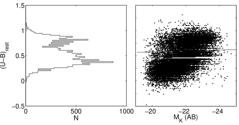
Figure 1: Rest Frame $(U-B)$ colours for UDS galaxies between $0.75<z<1.75$. Shown as a histogram and as a function of absolute K-band magnitude. The division between red and blue is shown, using the red-sequence slope derived by Hartley et al. (2010).

The galaxy sample used here is primarily based on selection in the K-band image, upon which we impose a cut at $K_{AB}$=23 to minimise photometric errors and spurious sources and also to ensure a high level of completeness ($\simeq$100 per cent) and reliable photometric redshifts (see Cirasuolo et al. 2010; Hartley et al. 2010). Bright stars are trivially removed from the combined catalogue by excluding objects on a stellar locus defined by 2-arcsec and 3-arcsec apertures, which is effective to $K<18.1$. The fainter stars are removed using a $(B-z^{\prime})-(z^{\prime}-K)$ diagram (Daddi et al., 2004) and the criterion $(z^{\prime}-K)<0.3~{}(B-z^{\prime})-0.5$. These cuts and careful masking of bright saturated stars and surrounding contaminated regions leave 33,765 galaxies in our sample.

2.2 Photometric Redshifts

The magnitudes from the DR3 catalogue were used to determine photometric redshifts and stellar ages by $\chi^{2}$ minimisation using a large set of templates. This was performed with a code based largely on the HYPERZ package (Bolzonella et al., 2000) using both average local galaxy SEDs and templates from the K20 survey. Six SEDs of observed starbursts from Kinney et al. (1996) were also used to improve the characterisation of young blue galaxies. This yeilded photometric redshifts with a $\delta$z/(1+z)=0.008 with a standard deviation of $\sigma$=0.034 after the exclusion of outliers (for more detail see Cirasuolo et al. 2007; Cirasuolo et al. 2010 and references within). This also provided rest frame magnitudes and colours, of which the rest frame $(U-B)$ and $K$-band absolute magnitude are utilised here. Sources with an unacceptable fit ($\chi^{2}>15$) are removed from our sample as these are likely to be unreliable. This removes 4$\%$ of the galaxy sample, the majority of these are either QSOs (36%), cross-talk (26%) or the minor members of pairs or mergers (23%), with the remainder consisting largely of objects with very low surface brightness. The fraction of otherwise useful objects rejected is therefore $<$0.6$\%$.

2.3 Passive Sample

To define a passive galaxy subset with minimal contamination from dusty star forming objects we use a subset of galaxies outlined in Hartley et al. (2010). Templates were used to fit either an instantaneous burst parameterised by an age, or an exponentially decaying star-formation rate parameterised by an age and $\tau$, the e-folding time in the exponentially declining star-formation rate, such that,

$$SFR=SFR_{0}\times e^{-age/\tau}$$ (1)

where $SFR$ is the star-formation rate at the time of observation and $SFR_{0}$ was the initial value. We define a conservative passive sample as galaxies that are simultaneously old (age$>$1Gyr) and have ongoing star formation with $SFR\leq 0.1\%$ of $SFR_{0}$, and a star forming sample with $SFR\geq 10\%$ of $SFR_{0}$, with 3947 and 22,158 galaxies in each sample respectively.

To define the red sequence we performed a $\chi^{2}$ minimisation to fit an equation of the form $(U-B)=a\times M_{K}+b$  to the old, burst galaxies, defining the red sample to be all galaxies within 3$\sigma$ of this fit (see Hartley et al. (2010) for a more detailed description). In this work, to separate red and blue galaxies, we use the red-sequence slope from Hartley et al. (2010) but choose the division between the two populations to fit the minimum in the overall colour bimodality (as shown in the histogram in Figure 1). This leads to a dividing line in the colour-magnitude diagram as follows:

$$(U-B)=-7.09\times 10^{-3}M_{K}+0.52$$ (2)

This boundary was found to separate the red and blue populations effectively to z$\sim$1.75. At higher redshift the bimodality in galaxy colours is less clear, which may in part be due to photometric errors. A full examination of this issue and the evolution of the red sequence will be presented in Cirasuolo et al. (in prep). Previous studies have found evidence for an evolution in the location of the red sequence with redshift (e.g Brammer et al. 2009). For simplicity we choose not to model the red sequence in such detail and instead use the fixed colour selection boundary given above. We note, however, that using an evolving boundary made no significant difference to any of the conclusions presented in this work.

Table 1 shows the resulting number of red and blue galaxies assigned to each photometric redshift bin, including the conservative subsamples of passive and actively star-forming galaxies.

3 Environmental Measurement

We used two methods to calculate galaxy environment: Counts in an Aperture and $n$th Nearest Neighbour. In both methods all the galaxies within a photometric redshift bin are collapsed down onto a 2D plane and the redshift information within the bin is not utilised any further. In the aperture method apertures of 1Mpc, 500kpc and 250kpc diameter (physical) are placed on each galaxy and the number of galaxies within that aperture are counted (N${}^{Aper}_{g}$). A sample of $\sim$100,000 random galaxies are then put down in the unmasked regions and the number of randoms within the aperture are counted (N${}^{Aper}_{r}$). The number of galaxies within the aperture is then normalised to give the final density measurement, $\rho/\rho_{r}$:

$$\frac{\rho}{\rho_{r}}=\frac{N^{Aper}_{g}}{N^{Aper}_{r}}\times\frac{N^{Tot}_{r}}{N^{Tot}_{g}}$$ (3)

where N${}^{Tot}_{r}$ and N${}^{Tot}_{g}$ are then total number of random points and galaxies respectively, so that $\rho/\rho_{r}$=1 corresponds to a density consistent with that of a random distribution of galaxies. This method was chosen to be the basis of this work as it is conceptually simple, and as concluded by Cooper et al. (2005), this technique has a distinct advantage in fields masked by a large number of holes. The nearest neighbour method would require the exclusion of a large fraction of data close to holes and field edges.

The $n$th nearest neighbour method was first employed by Dressler (1980), this calculates the distance to the $n$th nearest galaxy, $D_{n}$ in Mpc and is expressed here as a surface density,

$$\Sigma_{n}=\frac{n}{\pi D_{n}^{2}}$$ (4)

The surface density, $\Sigma_{n}$ is then renormalised such that,

$$\delta_{n}={\frac{\Sigma_{n}}{\bar{\Sigma}}}$$ (5)

where $\bar{\Sigma}$ is the median density of galaxies within the field. To reduce the effect of the edges, the distance to the nearest edge was calculated and if this was less than the distance to the third nearest neighbour then the object was removed from the sample. This method was only used in this work to test the primary findings of the aperture method. The results are presented in the appendix.

4 Results

Below we explore the relationship between galaxy colours and environment as a function of redshift. Relatively broad redshift bins are used to minimise the contamination due to photometric redshift errors. These sources of uncertainty are explored further in section 5.

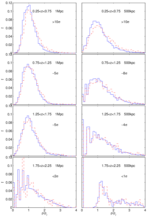
Figure 2: Histograms of the density of galaxies within 1Mpc and 500kpc diameter apertures compared to a random sample for red (dashed line) and blue (thick line) galaxies. The $\sigma$ values are obtained by performing a KS test, representing the significance in rejecting the null-hypothesis that the samples are drawn from the same underlying population.

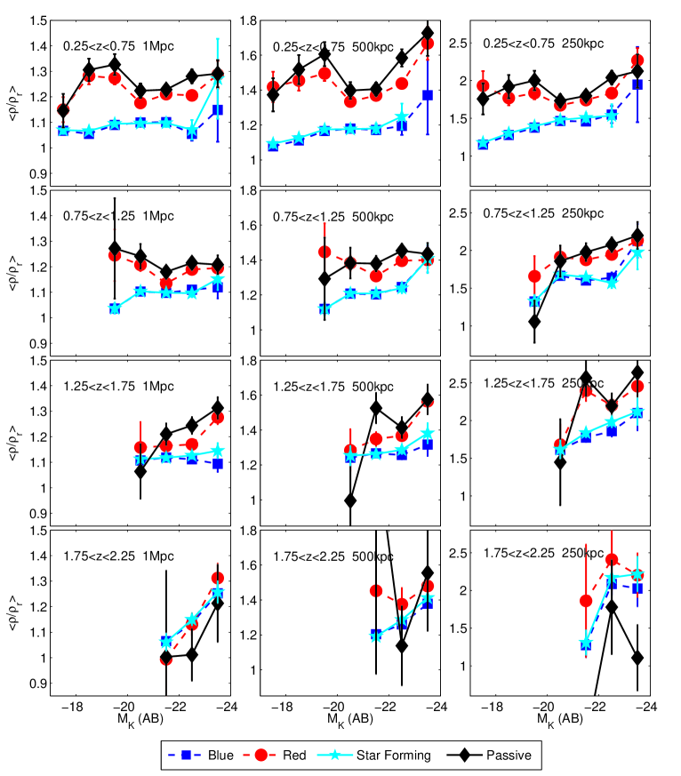
Figure 3: The average galaxy overdensity as a function of K-band luminosity, displayed in four redshift bins (top to bottom) and using projected apertures of diameter 1Mpc, 500kpc and 250kpc (three columns). Galaxies are displayed in red, blue, passive and star-forming subsets, as defined in Section 2. Note the change in scale for each column. The environments are defined so that $\rho/\rho_{r}$=1 corresponds to a density consistent with that of a random distribution of galaxies.

	$0.25<z<0.75$	$0.75<z<1.25$	$1.25<z<1.75$	$1.75<z<2.25$
Red	3,469	3,500	2,565	481
Blue	7,367	7,255	4,674	1,711
Passive	1,623	1,395	722	87
Star-forming	6,938	6,741	5,048	1,817

Table 1: Table showing the number of galaxies in each sample and in each redshift range, including our conservative subsets of passive and actively star-forming galaxies.

4.1 Red and Blue Environments

Figure 2 shows histograms of galaxy environments within two apertures of 1Mpc and 500kpc diameter. These are divided into four redshift bins between $z=0.25$ and $z=2.25$ and into red and blue populations. A KS-test was performed on the samples to assess the difference between the red and blue populations, with all but the final redshift bin showing highly significant differences between the two populations. In the first three redshift bins we can exclude the null hypothesis that the red and blue galaxies are drawn from the same underlying population with a significance in excess of 5$\sigma$ significance, falling to $<$2$\sigma$ and $<$1$\sigma$ significance at $z>1.75$.

Figure 3 is a plot of the mean density of red, blue, passive (black) and star forming (cyan) galaxies in bins of absolute K-band magnitude. Error bars are derived from the error on the mean density of galaxies within a given bin. Sources of error are explored further in Section 5. The passive and star forming galaxies are defined in Section 2. As before they are plotted in four redshift bins but with an additional 250kpc aperture. This plot illustrates that red and/or passive galaxies reside in significantly denser environments than blue and/or star-forming galaxies from the present day to $z\sim 1.5$, and this difference is apparent at all luminosities. This is comparable to what has been found in the local universe by other studies (Kauffmann et al. 2004; van Der Wel et al. 2008).

Figure 3 also shows that passive galaxies (shown in black) follow a similar density profile to red galaxies but are on average in slightly denser environments. This supports the conclusion that passive galaxies within the red population are responsible for the enhanced environments compared to blue star-forming objects. The environments of galaxies that were red but not in the strict ‘passive’ sample were also investigated and these were found to lie in-between the red and blue galaxy environments, as would be expected (these are not shown for clarity). The actively star-forming galaxies exhibit the same environmental dependence as the blue galaxies, following the same luminosity-density profile.

In addition to the clear separation of red and blue galaxies, we also find a general trend of increasing galaxy density with luminosity, particularly for blue galaxies and on smaller scales. Inspecting the two intermediate redshift bins in Figure 3, on scales below $500$kpc we find that the most luminous blue galaxies appear to inhabit environments approaching those of red/passive galaxies. These results are consistent with the findings of Cooper et al. (2007), who observed a strong increase in local density with luminosity for blue galaxies at $z\sim 1$. Our results appear to extend these findings to higher redshift, suggesting that the epoch $1<z<2$ represents a key period of transformation of massive galaxies from the blue cloud onto the passive red sequence.

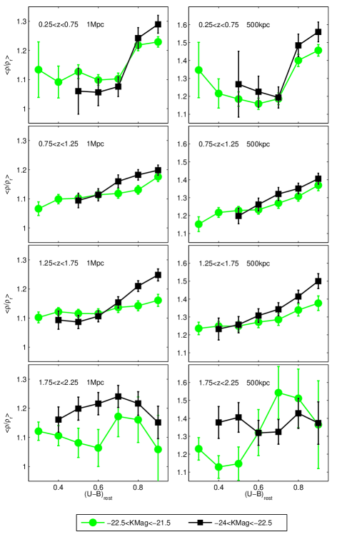
Figure 4: The average galaxy density in a 1Mpc and 500kpc diameter apertures compared to a random sample as a function of $(U-B)$ rest frame colour. We separate high (black) and low (green) luminosity subsets. Note the change in y-axis values between the two different aperture sizes.

4.2 Colour-Density Relation

In Figure 4 we display average density as a function of $(U-B)$ rest-frame colour, with faint (-22.5$<M_{K}<$-21.5) and luminous (-24$<M_{K}<$-22.5) objects shown in green and black respectively. This shows a clear trend for galaxies below z$\sim$2, with redder galaxies occupying denser average environments. In the lowest redshift bin this change occurs very abruptly at the boundary in the colour bimodality at $(U-B)_{rest}\sim$0.7 (see Figure 1). There is also a general trend for more luminous galaxies to occupy denser environments.

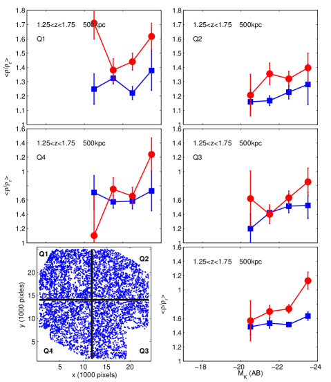
Figure 5: Showing the density of red and blue galaxies against K-band luminosity in four quadrants of the UDS field shown in the bottom left, using median values of x and y to calculate the position of the centre. The overall result for the field at 1.25$<$z$<$1.75 is shown in the bottom right with the error bars calculated from the error on the mean of the four quadrants, to give an estimate of the cosmic variance.

In summary, we have found strong evidence that red galaxies are on average found in denser local environments than blue galaxies, extending the comparison to a higher redshift than any previous study. Cooper et al. (2007) probed up to $z\sim 1.3$, finding that red and blue galaxies at this redshift occupy indistinguishable environments. In contrast we find that there is a significant difference between red and blue galaxies between $1.25<z<1.75$ (see Figures 2 and 3). This difference is likely to be due to our method of selecting galaxies from deep infrared imaging. Very red, passive galaxies will have been missed from the R-band selected candidates used in the DEEP2 study. This selection effect can be quantified using our UDS sample. Considering only the most luminous galaxies (M_K$\leq$-22.5) in the redshift range 1$<$z$<$1.3, if we impose the selection criteria of DEEP2 (R_AB$\leq$24.1) we find that 75% of red galaxies would be missed compared to only 20% of the blue sample. At fainter luminosities virtually no red/passive galaxies are selected.

5 Investigating Sources of Error

In this section we conduct a number of tests to investigate various source of systematic uncertainty. We attempt to quantify the cosmic variance in our data by dividing the survey into four quadrants. A volume limited study of the brighter galaxies is also performed, to allow a clearer comparison between different redshift bins. Finally we investigate the effects of photometric redshift errors using Monte Carlo simulations.

5.1 Cosmic Variance

To attempt to quantify the effects of cosmic variance on our results we divide the UDS field into four quadrants. The median values of the $x$ and $y$ positions of the galaxies were used to divide the field, to ensure that the number of galaxies in each quadrant was comparable. The results for the galaxies in the redshift range 1.25$<$z$<$1.75 are shown in Figure 5. The average density versus K-band absolute magnitude is shown for the four quadrants, with the bottom left panel showing the projected distribution in the field. The lower right panel shows the original result from Figure 3 (red and blue only) but with the error bars calculated from the error on the mean of the densities in the four quadrants in each magnitude bin. It can be seen that the distinction between red and blue galaxy environments remains, although there are clearly significant variations across the field. We conclude that while field variance is clearly present in these data the primary findings remain robust. Similar conclusions were drawn from other redshift bins and on other scales, which are not shown in the interests of brevity.

As a cautionary remark, however, we note that strictly speaking we have only tested the internal field variance, since despite the relatively wide field of the UDS ($50\times 50$ comoving Mpc at $z\sim 1$) we may nevertheless be prone to large-scale cosmic variance due to unusual superstructures (Somerville et al. 2004). Testing against such effects will require further wide-area infrared surveys, such as the forthcoming VIDEO and Ultra-VISTA surveys.

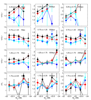
Figure 6: As Figure 3, but using only the brightest galaxies with M${}_{K}\leq$-22 (AB) as tracers of galaxy density. Note the change in y-axis values between the three different aperture sizes

5.2 Volume-Limited Sample

Our measurement of environmental density is based on a flux limited survey, so by definition we are using fainter galaxies to define environments at low redshift. To investigate the influence of this systematic effect we reduced the sample to only the brightest galaxies with $M_{K}\leq$-22 (AB) and repeated the environmental analysis using this volume-limited sample. This allows the galaxies to be used as tracers in the measure of environment over the same range in luminosity at all redshifts, to allow a fairer comparison between epochs. The results are shown in Figure 6, where the average density versus K-band luminosity is shown for comparison with the flux-limited study in Figure 3. As expected, the volume-limited study is much noisier (particularly at low redshift) but the results are consistent with the primary findings of Section 4. Red and/or passive galaxies are found to occupy denser environments on average to $z\sim 1.5$.

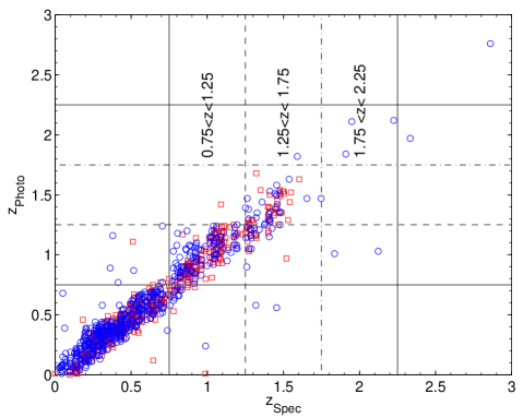
Figure 7: Plot of the reliable spectroscopic redshifts against photometric redshifts, highlighting the three highest redshift bins, 0.75$<$z$<$1.25, 1.25$<$z$<$1.75 and 1.75$<$z$<$2.25, with AGN and radio galaxies removed. The red squares and blue circles indicate the red and blue galaxies respectively, as defined in section 2.2.

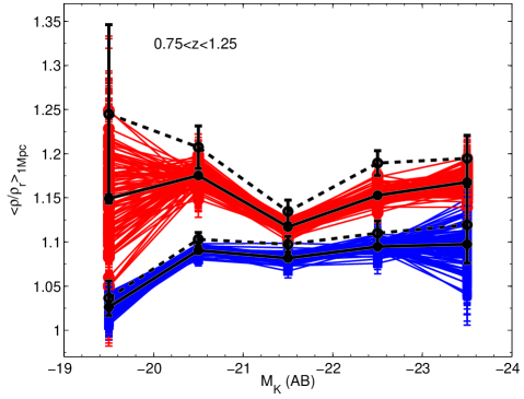
Figure 8: Monte Carlo simulation showing the effect of the photo-z errors on our measurement of galaxy overdensity, based on 100 simulations. The thick black line shows the average of the simulations and the dashed black line shows the original result for 0.75$<$z$<$1.25 from Figure 3.

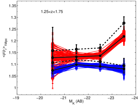
Figure 9: As Figure 8 but for the 1.25$<$z$<$1.75 bin.

5.3 Monte Carlo Simulations

Monte Carlo simulations were conducted to investigate the effect of photometric redshift errors on our results, explicitly allowing for the effects of outliers and catastrophic errors. Such errors would generally dilute differences in galaxy environments, but could potentially introduce fake overdensities if a large fraction of low-redshift structure is incorrectly assigned to a higher redshift bin. We note, of course, that the effects of photo-z errors are already present in the data, so these simulations can only provide an indication of the magnitude of the shifts due to these effects.

The distribution of spectroscopic versus photometric redshifts used in this field are shown in Figure 7, with spectroscopic redshifts derived from a variety of sources (Yamada et al. 2005; Simpson et al. 2006; Akiyama et al., in prep; Simpson et al., in prep; Smail et al., in prep) as outlined in Cirasuolo et al. (2010). We use the distribution in each redshift bin (higher redshift bins indicated in Figure 7) to estimate the fraction of galaxies incorrectly reassigned from one redshift bin to another. For simplicity two categories were adopted: ‘catastrophic’ errors were defined as those with $\delta z>0.25$, while others are classified as ‘normal’. In the absence of catastrophic errors we expect $>99.9\%$ of galaxies to show $\delta z<0.25$ at $z\sim 1$ (Cirasuolo et al. 2010). The resulting fractions were then randomly applied to the full sample, shifting galaxies into new bins to simulate the effect of photometric redshift errors (‘normal’ and ‘catastrophic’).

This was repeated 100 times per redshift bin. Results are displayed for the redshift bins $0.75<z<1.25$ (Fig.8) and $1.25<z<1.75$ (Fig.9). These simulations demonstrate that photometric redshift errors tend to dilute the distinction between the red and blue populations rather than introduce fake differences. The resulting additional sources of error in galaxy density are comparable to the errors on the mean displayed previously. Only in highest redshift bin ($z>1.75$) do the simulated populations introduce significant extra scatter (not shown). Given these findings, and the lack of spectroscopic redshifts at $z\sim 2$, we urge caution in interpreting our preliminary results in this highest redshift bin. At lower redshifts, however, the environmental differences appear robust.

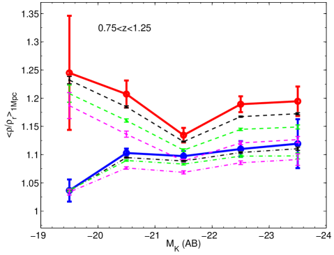
Figure 10: The results of Monte Carlo simulations based on the extreme scenario in which all incorrectly assigned photometric redshifts lead to blue galaxies being incorrectly classified as red, and vice versa. The original measures of environment for red galaxies and blue galaxies as a function of luminosity are shown as thick red and blue lines. Black dashed (dot-dashed) lines show the results of Monte Carlo simulations for the red (blue) populations respectively. The corresponding green and magenta lines illustrate the influence of doubling and tripling the number of incorrectly assigned galaxies.

Noting that we have only 97 spectroscopic redshifts in the redshift bin 1.25$<z<$1.75 (with 64 between 1.25$<z_{photo}<$1.75), where environmental differences appear to be very significant, we ran additional simulations using only half of the spectroscopic sample. The results were very similar to Figure 9, indicating that we are not suffering from low number statistics.

As an additional test, we conduct further Monte Carlo simulations to investigate the effects of contamination of the blue galaxies by the red population and vice versa. These simulations were motivated by the worry that incorrect redshifts may inevitably lead to errors in the resulting restframe $(U-B)$ colours. We adopt an extreme approach by simulating 100% misclassification, using the contaminating fractions outlined above but moving only blue galaxies into the red sample and vice versa. We find that these simulations have the effect of diluting the environment for both red and blue simulations, but once again are insufficient to influence any of the results previously presented. To investigate further, the contaminating fractions are artificially increased to double and triple the maximal contamination indicated by spectroscopic redshifts. These only serve to further reduce the average galaxy densities. Results for the $0.75<z<1.25$ bin are illustrated in Figure 10, and similar results are found for all other redshift bins.

We conclude that photometric redshift errors (including catastrophic errors) have only served to dilute the differences in environment, but an unrealistic proportion of misclassified galaxies are required to significantly influence our primary findings.

6 Conclusions

In this paper we have presented a study of the environment of over 33,000 K-band selected galaxies between 0.25$<$z$<$2.25. We have used a simple measurement of projected galaxy overdensities to study the environments of galaxies divided into red and blue based on rest frame $(U-B)$ colours, as well as using ‘passive’ and ‘star-forming’ galaxies from template fitting. We attempt to quantify the effects of cosmic variance, photometric redshift errors and flux-limit biases on the resulting environmental measurements. We find the following principle results:

1. We find a strong relationship between rest-frame $(U-B)$ colour and galaxy environment to $z\sim 1.5$, with red galaxies residing in significantly denser environments than blue galaxies on scales below $1$Mpc. These results are robust to the effects of field variance, flux-limit biases and photometric redshift errors. The environments appear indistinguishable by $z\sim 2$, but the current lack of spectroscopic redshifts at this epoch does not allow a robust test of this tantalising signal at present.

2. Selecting ‘passive’ and ‘star-forming’ galaxies using template fitting yields consistent results, with the passive subset occupying slightly denser environments than the global red population at all epochs. We conclude that the passive subset of the red galaxies are responsible for the enhanced environments compared to blue galaxies.

3. On small scales ($<0.5$ Mpc) we find evidence for a positive correlation between galaxy K-band luminosity (a good proxy for stellar mass) and local density. This trend is particularly clear for star-forming and blue galaxies, with the most luminous blue galaxies at $z\sim 1-2$ showing average environments comparable to passive red galaxies. These findings appear in very good agreement with the findings of Cooper et al. (2007) at $z\sim 1$. These results are consistent with the identification of high-z galaxies in transition to the red sequence in the densest environments.

To improve on this study, we note that the UDS imaging programme will continue at UKIRT until 2012 and ultimately probe $\sim 1$ magnitude deeper than the data used in this work. This will be sufficient to detect $L^{*}$ galaxies to $z\sim 5$ in addition to tens of thousands of sub-$L^{*}$ galaxies at lower redshift. Furthermore, an ongoing ESO Large Programme (UDSz) will soon transform the UDS project with the addition of $\sim 3000$ galaxy spectra. This will increase the number of UDS spectroscopic redshifts at $z>1.5$ by an order of magnitude, which we expect to dramatically improve the reliability of photometric redshifts and allow us to extend our study of galaxy environments and large-scale structure to the crucial epoch when the galaxy red sequence is first established.

Appendix: Nearest Neighbour method

In this appendix we use the nth nearest neighbour method as an alternative environmental estimator, to provide a test of the results presented earlier and to allow comparison with previous work (e.g. Cooper et al. 2007). The nth nearest neighbour was calculated for all the galaxies as a function of absolute magnitude, using the method outlined in Section 3. The value of n is chosen to probe the same mean scale as the apertures method. The results are shown in Figure 11), which appear globally consistent with those derived by the aperture method.

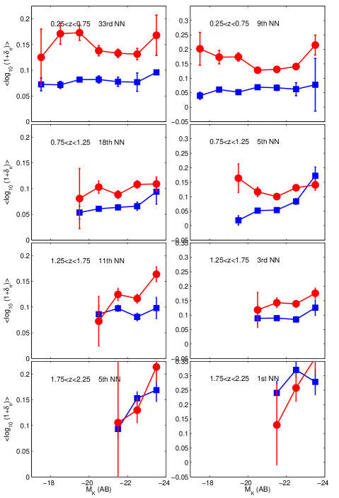
Figure 11: The nearest neighbour density of red and blue galaxies with the nearest neighbour chosen so that the mean distance probed was a diameter of 1Mpc and 500kpc in each redshift bin.

References

- Baldry et al. (2004) Baldry I.K. et al., 2004, ApJ, 600, 681
- Balogh et al. (2004) Balogh M. et al., 2004, MNRAS, 348, 1355
- Bamford et al. (2008) Bamford S.P. et al., 2008, MNRAS, 393, 1324
- Bell et al. (2004) Bell E.F et al., 2004, ApJ, 608, 752
- Benson (2005) Benson, A.J., 2005, Royal Society of London Philosophical Transactions Series A, 363, 695
- Birnboim et al. (2003) Birnboim Y., Dekel A., 2003, MNRAS, 345, 349
- Blanton et al. (2005) Blanton, M.R., Eisenstein D., Hogg D.W., Schlegel D.J., & Brinkmann J., 2005, ApJ, 629, 143
- Bolzonella et al. (2000) Bolzonella M., Miralles J.-M., & Pelló R., 2000, A&A, 363, 476
- Brammer et al. (2009) Brammer G.B., et al., 2009, ApJ, 706, L173
- Casali et al. (2007) Casali M. et al., 2006, A&A, 437, 777
- Cassata et al. (2008) Cassata P., et al., 2008, A&A, 483, L39
- Cirasuolo et al. (2007) Cirasuolo M. et al., 2007, MNRAS, 380, 585
- Cirasuolo et al. (2010) Cirasuolo, M. et al., 2010, MNRAS, 401, 1166
- Cooper et al. (2005) Cooper M.C. et al., 2005, ApJ, 634, 833
- Cooper et al. (2006) Cooper M.C. et al., 2006, MNRAS, 370, 198
- Cooper et al. (2007) Cooper M.C. et al., 2007, MNRAS, 376, 1445
- Cowie et al. (1996) Cowie L.L., Songaila A., Hu E.M. Cohen J. G., 1996, ApJ, 112, 839
- Cucciati et al. (2006) Cucciati. O. et al., 2006, A&A, 458, 39
- Daddi et al. (2003) Daddi E. et al., 2003, ApJ, 588, 50
- Daddi et al. (2004) Daddi E., Cimatti A., Renzini A., Fontana A., Mignoli M., Pozzetti L., Tozzi P. Zamorani G., 2004, ApJ, 617, 746
- Davis et al. (2003) Davis M. et al., 2003, Proc. SPIE, 4834, 161
- Dekel & Birnboim. (2006) Dekel A., & Birnboim Y., 2006, MNRAS, 368, 2
- Dressler (1980) Dressler A., 1980, ApJ, 236, 351
- Elbaz et al. (2007) Elbaz. D. et al., 2007, A&A, 468, 33
- Farouki et al. (1981) Farouki R., Shapiro, S.L., 1981, ApJ, 243, 32
- Foucaud et al. (2007) Foucaud, S. et al., 2007, MNRAS, 376, L20
- Furusawa et al. (2008) Furusawa H. et al., 2008, ApJS, 176, 1
- Gunn et al. (1972) Gunn J.E., Gott J.R., 1972, ApJ, 176, 1
- Hartley et al. (2008) Hartley W.G., et al., 2008, MNRAS, 391, 1301
- Hartley et al. (2010) Hartley W.G., et al., 2010, MNRAS, 407, 1212
- Hogg et al. (2003) Hogg D.W., et al., 2003, ApJ, 585, L5
- Kauffmann et al. (2004) Kauffmann G. et al., 2004, MNRAS, 353, 713
- Kriek et al. (2008) Kriek M., van der Wel A., van Dokkum P.G., Franx M.,& Illingworth G.D., 2008, ApJ, 682, 896
- Kinney et al. (1996) Kinney A.L., Calzetti D., Bohlin R.C., McQuade K., Storchi-Bergmann T., & Schmitt H.R., 1996, ApJ, 467, 38
- Lawrence et al. (2007) Lawrence A. et al., 2007, MNRAS, 379, 1599
- Le Fèvre et al. (2005) Le Fèvre O. et al., 2005, , 439, 877
- Oemler (1974) Oemler A., 1974, ApJ, 194, 1
- Poggianti et al. (2009) Poggianti B. M. et al., 2009, ApJ, 693, 112
- Quadri et al. (2007) Quadri R. et al., 2007, ApJ, 654, 138
- Simpson et al. (2006) Simpson C. et al., 2006, MNRAS, 372, 741
- Springel et al. (2005) Springel V., Di Matteo T., Hernquist, L., 2005, ApJ, 620, L20
- Toomre et al. (1972) Toomre A. , Toomre J., 1972, ApJ, 178, 623
- van Der Wel et al. (2008) van Der Wel A. et al., 2008, ApJ, 675, 13
- White et al. (1991) White S.D.M., Frenk C.S., 1991, ApJ, 379, 52
- Williams et al. (2009) Williams R.J., Quadri R.F., Franx M., van Dokkum P.,& Labbé I., 2009, ApJ, 691, 1879
- Yamada et al. (2005) Yamada T. et al., 2005, ApJ, 634, 52
- York et al. (2002) York D.G. et al., 2000, AJ, 120, 1579