Dynamical Rare event simulation techniques for equilibrium and non-equilibrium systems

1 Introduction

Molecular dynamics (MD) is the ultimate method to gain detailed atomistic information of dynamical processes that are difficult to access experimentally. However, an important bottleneck of atomistic simulations is the limited system- and timescales. Depending on the complexity of the forcefields (Ab Initio MD being extremely more expensive than classical MD) systems typically consist of 100 to 100000 molecules that can be simulated for a period of nanoseconds till microseconds. Therefore, many activated processes can not be studied using brute-force MD because the probability to observe a reactive event within reasonable CPU time is basically zero. Typical examples are protein folding, conformational changes of molecules, cluster isomerizations, chemical reactions, diffusion in solids, ion permeation through membranes, enzymatic reactions, docking, nucleation, DNA denaturation, and other types of phase transitions. If these processes are treated with straightforward MD, the simulations will endlessly remain in the reactant states. Still, if an event would happen, it can go very fast. The time it actually takes to cross the barrier is usually much shorter than this computational accessible timescale. Therefore, rare event algorithms aim to avoid the superfluous exploration of the reactant state and to enhance the occurrence of reactive events. The methods that I will discuss are the reactive flux (RF) method [1, 2] and the more recent algorithms that originate from the transition path sampling (TPS) [3, 4, 5, 6, 7] methodology. These comprise the transition interface sampling (TIS) [8] and the replica exchange TIS (RETIS) [9, 10], which are successive improvements on the way reaction rates were determined in the original TPS algorithm. Partial path TIS (PPTIS) [11] is an approximative approach in order to reduce the simulated path length for the case of diffusive barrier crossings. PPTIS is similar to Milestoning [12], that was developed simultaneously and independently from PPTIS. For non-equilibrium systems, the Forward Flux Sampling (FFS) was designed [13]. This method is based on the TIS formalism, but does not require prior knowledge on the phasepoint density. All these methods have in common that they aim to simulate true molecular dynamics trajectories at a much faster rate than naive brute force molecular dynamics. I will discuss the advantages and disadvantages of the different methodologies and introduce a few new relations and derive some known relations using a nonstandard approach. The descriptions of these methods given here are far from complete and, therefore, to obtain a more complete picture of the path sampling techniques I would like to recommend some very recent complementary reviews on these methodologies,[14, 15, 16, 17]. In the end, I compare all the methods by applying them on a simple, though tricky, test system. The outcome illustrates some important pitfalls for the non-equilibrium methods that have no easy solution and show that caution is necessary when interpreting their results.

2 Reactive Flux Method

Low dimensional systems, such as chemical reactions in the gas phase, are usually well described by Transition State Theory (TST). TST assumes that the transitions from reactant to product state always follow a path on the potential energy surface such that it passes the barrier nearby the transition state (TS). The TS refers to the point on the energy barrier having to the lowest possible potential energy difference, with respect to the reactant state, that any trajectory must overcome in order to reach the product state. In this description, TS corresponds to a unstable stationary point on the potential energy surface having one imaginary frequency (saddle point). In condensed systems, the saddle-point of the full potential energy surface is usually less meaningful. For instance, if we would consider the dissociation of NaCl in water, the TS would correspond to a state where the inter-ion distance is fixed to a critical value while all surrounding water molecules are full frozen into an icy state. It is needless to say that this does not correspond to our daily experience when dissolving some pinch of salt in a glass of water. TST can be generalized for higher dimensional systems using the free energy instead of the potential energy. The TS is then no longer a single point, but a multidimensional surface. In this case, the TST equation is determined by the free energy difference between the TS dividing surface and the reactant state. An important limitation of TST is that the free energy barrier depends on the selected degrees of freedom that are used to describe the free energy surface. In addition, TST implicitly assumes that any trajectory will cross the free energy barrier only once when going from reactant to product state. Kramers’ theory[18] provides an elegant and insightful approach to correct for correlated recrossings if these originate from the diffusive character of the dynamics. However, there are several other sources for recrossings. For instance, if the selected degrees of freedom are not well chosen, the barriers in the free energy landscape do not always correspond the barriers in the underlying potential energy surface which ultimately determine the dynamics. The reactive flux (RF) method is able to correct for recrossings regardless their origin and is very powerful when when TST is close but not sufficiently accurate.

The theory of the method originated from the early 1930s, far before the first applications of computers for molecular dynamics simulations [19]. After Wigner and Eyring introduce the concept of the TS and the TST approximation [20, 21], Keck [22] demonstrated how to calculate the dynamical correction, the transmission coefficient. This work has later been extended by Bennett [23], Chandler [24] and others [25, 26], resulting in a two-step approach. First the free energy as function of a single reaction coordinate (RC) is determined. This can be done by e.g. umbrella sampling (US) [27] or thermodynamic integration (TI) [28]. Then, the maximum of this free energy profile defines the approximate TS dividing surface and the transmission coefficient can be calculated by releasing dynamical trajectories from the top.

Traditionally, the equation for the dynamically corrected rate constant is derived by applying a small perturbation to the equilibrium state and invoking the fluctuation-dissipation theorem and Onsager’s relation [25, 1, 2]. However, as I will show here, there is an alternative derivation that naturally evolves to a formula for transmission coefficient that is probably more efficient that the standard one [23, 24].

There are several definitions for the rate constant $k_{AB}$ between two states $A$ and $B$, such as the transition probability per unit time, the inverse mean residence time in state $A$, or the inverse mean first passage time towards state $B$ [29]. However, all these different definitions become equivalent for truly exponential relaxation, which is the case whenever the stable states $A$ and $B$ are separated by large free energy barriers. If this is not the case, the rate constant becomes ill-defined. To start the derivation I will use the first definition, which can be expressed as follows:

$$k_{AB}=\lim_{{\mathrm{d}}t\rightarrow 0}\frac{1}{{\mathrm{d}}t}\frac{\textrm{number of states $A$ that transform into state $B$ within ${\mathrm{d}}t$}}{\textrm{number of states $A$}}$$ (1)

Let us denote $x=(r,v)$ the phasepoint which includes the positions $r$ and velocities $v$ of all particles in the system. We define the reaction coordinate $\lambda(x)$ which can be any function of $x$, though in practice it will generally only depend on $r$. The RC function should describe the progress of the reaction, but there is a lot of flexibility in designing this RC function.

We will assume that the collection of phasepoints $\{x|\lambda(x)=0\}$ defines the transition state dividing surface that separates region $A$ and $B$. For convenience, we will also assume that the RC will increase when going from $A$ to $B$. Considering the phenomenological equation 1, we can directly write down the reaction rate as

$$k_{AB}=\lim_{{\mathrm{d}}t\rightarrow 0}\frac{1}{{\mathrm{d}}t}\frac{\int{\mathrm{d}}x_{0}\,\theta\left(-\lambda\left(x_{0}\right)\right)\theta\left(\lambda\left(x_{{\mathrm{d}}t}\right)\right)\rho(x_{0})}{\int{\mathrm{d}}x_{0}\theta\left(-\lambda\left(x_{0}\right)\right)\rho(x_{0})}=\lim_{{\mathrm{d}}t\rightarrow 0}\frac{1}{{\mathrm{d}}t}\frac{\langle\theta\left(-\lambda\left(x_{0}\right)\right)\theta\left(\lambda\left(x_{{\mathrm{d}}t}\right)\right)\rangle}{\langle\theta\left(-\lambda\left(x_{0}\right)\right)\rangle}$$ (2)

where $x_{0}$ and $x_{{\mathrm{d}}t}$ are phasepoints at times $t=0$ and $t={\mathrm{d}}t$. $\rho(x)$ denotes the phasepoint density. For equilibrium statistics this is simply given by Boltzmann $\rho(x)=\exp(-\beta E(x))$ where $E$ the energy and $\beta=1/k_{B}T$, $T$ the temperature, and $k_{B}$ the Boltzmann constant. $\theta$ is the Heaviside-step function with $\theta(y)=0$ if $y<0$ and $\theta(y)=1$ otherwise. The brackets $\langle\ldots\rangle\equiv\int{\mathrm{d}}x\,\dots\rho(x)/\int{\mathrm{d}}x\,\rho(x)$ denote the ensemble average over the initial condition $x_{0}$. Eq. 2 is basically the TST expression of the rate, but written in a somewhat unusual form.

To transform this equation into the standard form, we can use $\lambda\left(x_{{\mathrm{d}}t}\right)=\lambda\left(x_{0}\right)+{\mathrm{d}}t\dot{\lambda}(x_{0})+{\mathcal{O}}({\mathrm{d}}t^{2})$, where the dot denotes the time derivative. If we neglect the second order terms, we can write for an arbitrary function $a(x)$:

$$\int{\mathrm{d}}x_{0}\,\theta\left(-\lambda\left(x_{0}\right)\right)\theta\left(\lambda\left(x_{{\mathrm{d}}t}\right)\right)a(x_{0})=\int{\mathrm{d}}x_{0}\,\theta\left(-\lambda\left(x_{0}\right)\right)\theta\left(\lambda\left(x_{0}\right)+{\mathrm{d}}t\dot{\lambda}\left(x_{0}\right)\right)a(x_{0})$$ (3)

Clearly, $\theta(-\lambda)\theta(\lambda+{\mathrm{d}}t\dot{\lambda})$ is only nonzero if $\dot{\lambda}>0$ and ${\mathrm{d}}t\dot{\lambda}<\lambda<0$. Instead of integrating over $x_{0}$, we will apply a coordinate transform such that we can integrate Eq. 3 over $\lambda,\dot{\lambda}$ and a remaining set coordinates $x_{0}^{\prime}$. Assume that $J(x_{0}^{\prime},\lambda,\dot{\lambda})$ is the corresponding Jacobian of this transformation. We can then integrate out the $(\lambda,\dot{\lambda})$ coordinates

$$\int{\mathrm{d}}x_{0}\,\theta\left(-\lambda\left(x_{0}\right)\right)\theta\left(\lambda\left(x_{0}\right)+{\mathrm{d}}t\dot{\lambda}\left(x_{0}\right)\right)a(x_{0})=\int{\mathrm{d}}x_{0}^{\prime}\int_{0}^{\infty}{\mathrm{d}}\dot{\lambda}\int_{-{\mathrm{d}}t\dot{\lambda}}^{0}{\mathrm{d}}\lambda\,a(x_{0}^{\prime},\lambda,\dot{\lambda})J(x_{0}^{\prime},\lambda,\dot{\lambda})$$ (4)

$$= \int{\mathrm{d}}x_{0}^{\prime}\int_{0}^{\infty}{\mathrm{d}}\dot{\lambda}\int_{-{\mathrm{d}}t\dot{\lambda}}^{0}{\mathrm{d}}\lambda\,\Big{\{}a(x_{0}^{\prime},0,\dot{\lambda})J(x_{0}^{\prime},0,\dot{\lambda})+\lambda\frac{\partial(a(x_{0}^{\prime},\lambda,\dot{\lambda})J(x_{0}^{\prime},\lambda,\dot{\lambda}))}{\partial\lambda}\Big{|}_{\lambda=0}+\ldots\Big{\}}$$

$$= \int{\mathrm{d}}x_{0}^{\prime}\int_{0}^{\infty}{\mathrm{d}}\dot{\lambda}\,\Big{\{}({\mathrm{d}}t\dot{\lambda})a(x_{0}^{\prime},0,\dot{\lambda})J(x_{0}^{\prime},0,\dot{\lambda})-\frac{1}{2}({\mathrm{d}}t\dot{\lambda})^{2}\frac{\partial(a(x_{0}^{\prime},\lambda,\dot{\lambda})J(x_{0}^{\prime},\lambda,\dot{\lambda}))}{\partial\lambda}\Big{|}_{\lambda=0}+\ldots\Big{\}}$$

$$= {\mathrm{d}}t\times\int{\mathrm{d}}x_{0}^{\prime}\int_{0}^{\infty}{\mathrm{d}}\dot{\lambda}\,\dot{\lambda}a(x_{0}^{\prime},0,\dot{\lambda})J(x_{0}^{\prime},0,\dot{\lambda})+\mathcal{O}({\mathrm{d}}t^{2})$$

where we applied a Taylor expansion in terms of $\lambda$ in the second line. Clearly, as

$$\int{\mathrm{d}}x_{0}\,\dot{\lambda}\left(x_{0}\right)\delta\left(\lambda\left(x_{0}\right)\right)\theta\left(\dot{\lambda}\left(x_{0}\right)\right)a(x_{0}) = \int{\mathrm{d}}x_{0}^{\prime}{\mathrm{d}}\dot{\lambda}{\mathrm{d}}\lambda\,\dot{\lambda}\delta(\lambda)\theta(\dot{\lambda})a(x_{0}^{\prime},\lambda,\dot{\lambda})J(x_{0}^{\prime},\lambda,\dot{\lambda})$$ (5)

$$= \int{\mathrm{d}}x_{0}^{\prime}\int_{0}^{\infty}{\mathrm{d}}\dot{\lambda}\,\dot{\lambda}a(x_{0}^{\prime},0,\dot{\lambda})J(x_{0}^{\prime},0,\dot{\lambda})$$

we have proven that

$$\lim_{{\mathrm{d}}t\rightarrow 0}\frac{1}{{\mathrm{d}}t}\theta\left(-\lambda\left(x_{0}\right)\right)\theta\left(\lambda\left(x_{{\mathrm{d}}t}\right)\right)=\dot{\lambda}\left(x_{0}\right)\delta\left(\lambda\left(x_{0}\right)\right)\theta\left(\dot{\lambda}\left(x_{0}\right)\right)$$ (6)

Using this expressing into Eq. 2, we obtain the standard form of the TST formula:

$$k_{AB}=\frac{\langle\dot{\lambda}\left(x_{0}\right)\delta\left(\lambda\left(x_{0}\right)\right)\theta\left(\dot{\lambda}\left(x_{0}\right)\right)\rangle}{\langle\theta\left(-\lambda\left(x_{0}\right)\right)\rangle}$$ (7)

It is often very convenient to switch back to the other formalism, Eq. 2, as some relations follow more naturally from this expression, especially in path sampling simulations where ${\mathrm{d}}t$ can simply be taken as the MD timestep. The TST approach rewrites Eq. 7 into two factors

$$k_{AB}=\frac{\langle\dot{\lambda}\left(x_{0}\right)\delta\left(\lambda\left(x_{0}\right)\right)\theta\left(\dot{\lambda}\left(x_{0}\right)\right)\rangle}{\langle\delta\left(\lambda\left(x_{0}\right)\right)\rangle}\times\frac{\langle\delta\left(\lambda\left(x_{0}\right)\right)\rangle}{\langle\theta\left(-\lambda\left(x_{0}\right)\right)\rangle}\equiv R^{\rm TST}\times\frac{e^{-\beta F(0)}}{\int_{-\infty}^{0}{\mathrm{d}}\lambda\,e^{-\beta F(\lambda)}}$$ (8)

where the free energy $F$ is defined as $F(\lambda)\equiv-\ln\langle\delta(\lambda-\lambda(x))\rangle/\beta$. Numerous techniques exist to calculate the free energy profile along the barrier region [27, 28, 30, 31, 32, 33, 34, 35]. The kinetic term $R^{\rm TST}$ usually follows from a simple numerical or analytical integration. For instance, if the RC is a simple Cartesian coordinate of a target particle then $R^{\rm TST}=1/\sqrt{2\pi\beta m}$ where $m$ is the mass of the particle.

The TST expression neglects correlated fast recrossings and, therefore, overestimates the reaction rate. Recrossings can occur due to a diffusive motion on top of the barrier or by kinetic correlations when the kinetic energy of the RC is not dissipated. Another important source of recrossings is when the one-dimensional RC gives an incomplete description of the reaction kinetics [2]. To correct for recrossing we can apply the effective positive flux formalism which neglects the crossings that are not ”effective”. At each side of the barrier we define regions that are the stable regions $A$ and $B$. These might be smaller than the regions that we associate to the product and reactant state. Entering $A$ or $B$ implies that the system is committed to that side, i.e. it might leave region $A$ or $B$ shortly thereafter, but the chance to rapidly recross the barrier is of the same order as an independent new event. An effective positive crossing is then defined as the first crossing on the trajectory that makes the transition from $A$ to $B$ (See fig. 1). This leads to the effective positive flux expression for the reaction rate:

Figure 1: Definition of an effective positive crossing on a very long MD trajectory. The EPF algorithm will ignore all crossing with the TS dividing surface except one (black dot). These are the first crossing points with the TS dividing surface for the parts of the MD trajectory that start at $A$ and end at $B$ (without revisiting $A$ again).

$$k_{AB} = \lim_{{\mathrm{d}}t\rightarrow 0}\frac{1}{{\mathrm{d}}t}\frac{\langle\theta\left(-\lambda\left(x_{0}\right)\right)\theta\left(\lambda\left(x_{{\mathrm{d}}t}\right)\right)h^{b}_{A0}(x_{0})h^{f}_{BA}\left(x_{0}\right)\rangle}{\langle\theta\left(-\lambda\left(x_{0}\right)\right)\rangle}$$ (9)

$$= \frac{\langle\dot{\lambda}\left(x_{0}\right)\delta\left(\lambda\left(x_{0}\right)\right)\theta\left(\dot{\lambda}\left(x_{0}\right)\right)h^{b}_{A0}(x_{0})h^{f}_{BA}\left(x_{0}\right)\rangle}{\langle\theta\left(-\lambda\left(x_{0}\right)\right)\rangle}$$

where $h^{b/f}_{uv}(x_{0})$ detects whether a backward/forward time trajectory crosses or enters a certain interface/region $u$ before interface/region $v$. If this is true, the function is one. It is zero otherwise. In the second line we applied again equality 6. Naturally, the ensemble average $\langle\ldots\rangle$ should now not only integrate over the phasepoint $x_{0}$, but also sum over all possible trajectories backward and forward in time starting from $x_{0}$. The ratio between the exact expression (Eq. 9) and the transition state expression (Eq. 7) is the transmission coefficient: $k^{\rm exact}=\kappa k^{\rm TST}$ so that

$$\kappa = \frac{\langle\dot{\lambda}\left(x_{0}\right)\delta\left(\lambda\left(x_{0}\right)\right)\theta\left(\dot{\lambda}\left(x_{0}\right)\right)h^{b}_{A0}(x_{0})h^{f}_{BA}\left(x_{0}\right)\rangle}{\langle\dot{\lambda}\left(x_{0}\right)\delta\left(\lambda\left(x_{0}\right)\right)\theta\left(\dot{\lambda}\left(x_{0}\right)\right)\rangle}$$ (10)

$$= \frac{\langle\dot{\lambda}\left(x_{0}\right)\theta\left(\dot{\lambda}\left(x_{0}\right)\right)h^{b}_{A0}(x_{0})h^{f}_{BA}\left(x_{0}\right)\rangle_{\lambda=0}}{\langle\dot{\lambda}\left(x_{0}\right)\theta\left(\dot{\lambda}\left(x_{0}\right)\right)\rangle_{\lambda=0}}$$

Here the subscript $\lambda=0$ denotes an ensemble average on the TST dividing surface. Strictly speaking, the above expression is correct for any surface that separates the two stable states. However, the efficiency to calculate the above expression is significant better if $\kappa$ is maximized. Therefore, $\lambda=0$ should be defined on the top of the free energy barrier. If we assume that $\lambda(x)=\lambda(r)$ depends on configuration space only, the calculation requires to generate a representative set of configuration points on the TST surface. Then, we attribute to these points $r$ a randomized set of velocities taken from a Maxwellian distribution and integrate the equations of motion backward and forward in time. However, as $\theta\left(\dot{\lambda}\right)h^{b}_{A0}=0$ if $\dot{\lambda}<0$ or when the backward trajectory recrosses the TST dividing surface before entering $A$, only a very few trajectories need to be fully integrated in both time-directions until reaching stable states. It is surprising that the effective positive flux counting strategy is not so common. To our knowledge only two slightly different expressions of a transmission coefficient based on the effective positive flux have been proposed in Refs. [36, 37]. All other expressions in the literature do not avoid the counting of recrossings. In these algorithms, the final rate constant follows through cancellation of many negative and positive terms. For instance, the most popular formulation of the rate constant and transmission coefficient is the Bennett-Chandler (BC) expression that appears in many textbooks on molecular simulation [1, 2].

$$\tilde{k}_{AB}(t) = \frac{\langle\dot{\lambda}\left(x_{0}\right)\delta\left(\lambda\left(x_{0}\right)\right)\theta\left(\lambda\left(x_{t}\right)\right)\rangle}{\langle\theta\left(-\lambda\left(x_{0}\right)\right)\rangle}\Rightarrow$$

$$\tilde{\kappa}(t) = \frac{\langle\dot{\lambda}\left(x_{0}\right)\theta\left(\lambda\left(x_{t}\right)\right)\rangle_{\lambda=0}}{\langle\dot{\lambda}\left(x_{0}\right)\theta\left(\dot{\lambda}\left(x_{0}\right)\right)\rangle_{\lambda=0}}$$ (11)

Here, the reaction rate and transmission coefficient are expressed as time-dependent functions. However, the actual rate constant and transmission coefficient, which should not depend on time, follow from a plateau value of these time-dependent functions: $k_{AB}=\tilde{k}_{AB}(t^{\prime}),\kappa=\tilde{\kappa}(t^{\prime})$ with $\tau_{\rm mol}<t^{\prime}<\tau_{\rm rxn}$. In other words, $\tilde{k}(t)$ and $\kappa(t)$ will generally show oscillatory behavior at small $t$. However, after some molecular timescale $\tau_{\rm mol}$, the system will basically enter either region $A$ or $B$ (See fig. 1) after which we won’t expect any recrossing until reaching the actual relaxation time $\tau_{\rm rxn}>>\tau_{\rm mol}$. The equivalence between Eq. 11 and Eqs. 9, 10, can be shown by invoking $\theta\left(\lambda\left(x_{t^{\prime}}\right)\right)=h^{f}_{BA}(x_{0})$, Eq. 6, and its mirror equivalent $\lim_{dt\rightarrow 0}\theta(\lambda(x_{0}))\theta(-\lambda(x_{{\mathrm{d}}t}))/dt=-\dot{\lambda}(x_{0})\delta(\lambda(x_{0}))\theta(-\dot{\lambda}(x_{0}))$:

$$k = \tilde{k}(t^{\prime})=\frac{\langle\dot{\lambda}\left(x_{0}\right)\delta\left(\lambda\left(x_{0}\right)\right)\theta\left(\lambda\left(x_{t^{\prime}}\right)\right)\rangle}{\langle\theta\left(-\lambda\left(x_{0}\right)\right)\rangle}=\frac{\langle\dot{\lambda}\left(x_{0}\right)\delta\left(\lambda\left(x_{0}\right)\right)h^{f}_{BA}\left(x_{0}\right)\rangle}{\langle\theta\left(-\lambda\left(x_{0}\right)\right)\rangle}$$ (12)

$$= \frac{\langle\dot{\lambda}\left(x_{0}\right)\delta\left(\lambda\left(x_{0}\right)\right)\theta\left(\dot{\lambda}\left(x_{0}\right)\right)h^{f}_{BA}\left(x_{0}\right)+\dot{\lambda}\left(x_{0}\right)\delta\left(\lambda\left(x_{0}\right)\right)\theta\left(-\dot{\lambda}\left(x_{0}\right)\right)h^{f}_{BA}\left(x_{0}\right)\rangle}{\langle\theta\left(-\lambda\left(x_{0}\right)\right)\rangle}$$

$$= \lim_{{\mathrm{d}}t\rightarrow 0}\frac{1}{{\mathrm{d}}t}\left(\frac{\langle\theta\left(-\lambda\left(x_{0}\right)\right)\theta\left(\lambda\left(x_{{\mathrm{d}}t}\right)\right)h^{f}_{BA}\left(x_{0}\right)-\theta\left(\lambda\left(x_{0}\right)\right)\theta\left(-\lambda\left(x_{{\mathrm{d}}t}\right)\right)h^{f}_{BA}\left(x_{0}\right)\rangle}{\langle\theta\left(-\lambda\left(x_{0}\right)\right)\rangle}\right)$$

We have now transferred the BC expression in an unitary ensemble average; each phasepoint $x_{0}$ either returns 1, 0, or -1. Consider a very long MD trajectory with a timestep of ${\mathrm{d}}t$ (like the one in fig. 1). It is clear that any detailed-balance simulation method should sample each phasepoint $x_{0}$ on this trajectory equally often. As such, an unreactive $B\rightarrow B$ trajectory will always have an equal number of phasepoints returning $+1$ as $-1$. The $B\rightarrow B$ trajectories are therefore effectively not counted due to this cancellation. The phasepoints on the $A\rightarrow A$ trajectory are always zero due to the $h^{f}_{BA}$ characteristic function. Finally, any trajectory $A\rightarrow B$ always has one $x_{0}$ more that is +1 than -1. A more formal mathematical proof of the equivalence between Eq. 11 and Eq. 9 can be found in Ref. [38].

Whenever, there are a significant number of recrosssings, the BC formalism has obvious disadvantages. In general, we note that any averaging method counting only zero and positive values will show a faster convergence than one that is based on cancellation of positive en negative terms. Moreover, in the effective flux formalism many trajectories will be assigned as unreactive after just a few MD steps, thus reducing the number of required force evaluations. Another important advantage of the EPF formalism is that is generates a set of trajectories that are unambiguous interpretable as reactive or unreactive, while the BC scheme generates only forward trajectories of which some actually belong to unreactive $B\rightarrow B$ trajectories. Instead of integrating the equations of motion until reaching stable states, one can also use a time-dependent expression for the EPF [39] similar to Eq. 11.

There are several other formulations of the transmission coefficient (see [40]), but most of them rely on a cancellation between positive and negative flux terms. A comparative study of ion channel diffusion [41] showed that the algorithm based on effective positive flux expression was superior to the other transmission rate expressions. Moreover, it was as efficient as an optimized version of the more complicated method of Ruiz-Montero et al.[42]. The implementation of the EPF scheme is as simple as algorithms that are based on the BC transmission coefficient. Therefore, the EPF implementation of the RF method should in principal be preferred above the standard implementations that require cancellation.

3 Transition Path sampling

In the previous section, I showed how the standard transmission coefficient calculations can be improved using the effective positive flux expression. However, this approach can not fully eliminate the main bottleneck of the RF methods. If $\kappa<<1$ the number of trajectories that are required for sufficient statistics can be tremendous. In specific, if one is unable to find a proper RC, the overwhelming majority of trajectories that are released from the top of the barrier will be either $A\rightarrow A$ or $B\rightarrow B$ trajectories [2]. In practice, it has been discovered that finding a good RC can be extremely difficult in high dimensional complex systems. Notable examples are chemical reactions in solution, where the reaction mechanism often depends on highly non- trivial solvent rearrangements [43]. Also, computer simulations of nucleation processes use very complicated order parameters to distinguish between particles belonging to the liquid and solid phase. This makes it unfeasible to construct a single RC that accurately describes the exact place of cross-over transitions. As a result, hysteresis effects and low transmission coefficients are almost unavoidable.

This has been the main motivation of Chandler and collaborators [3, 4, 5, 6, 7] to devised a method that generates reactive trajectories without the need of a RC. This method, called transition path sampling (TPS), gathers a collection of trajectories connecting the reactant to the product stable region by employing a Monte Carlo (MC) procedure called shooting.

Suppose ${\bf x}$ is a path $\{x_{0},x_{{\mathrm{d}}t},x_{2{\mathrm{d}}t},\ldots,x_{n{\mathrm{d}}t}\}$ of $n$ timeslices. The statistical weight given to this path equals

$$P[{\bf x}]=\rho(x_{0})p(x_{0}\rightarrow x_{{\mathrm{d}}t})p(x_{{\mathrm{d}}t}\rightarrow x_{2{\mathrm{d}}t})\ldots p(x_{(n-1){\mathrm{d}}t}\rightarrow x_{n{\mathrm{d}}t})\hat{h}({\bf x})$$ (13)

where $\rho(x_{0})$ is the usual phasepoint density and $p(x_{j{\mathrm{d}}t}\rightarrow x_{(j+1){\mathrm{d}}t})$ is probability density that the MD integrator generates $x_{(j+1){\mathrm{d}}t}$ starting from $x_{j{\mathrm{d}}t}$. The characteristic function $\hat{h}({\bf x})$ equals 1 (otherwise 0) if a specific condition is fulfilled. For instance, one could imply that the trajectory ${\bf x}$ needs to start in state $A$ and end in state $B$.

By means of the shooting algorithm, TPS performs a random walk in path space to generate one trajectory after the other (See fig. 2). The first step of this approach consists of a random selection of one of the timeslices of the old path, called the shooting point. This timeslice is modified by making random modifications in the velocities and/or positions. Then, there is usually an acceptance or rejection step based on the energy difference between modified and unmodified shooting point. If accepted, the equations of motion are integrated forward and backward in time until a certain path length is obtained or until the condition function $\hat{h}({\bf x})$ can be assigned 0 or 1. In the last case the trial move will be accepted. Any rejection along this scheme implies that the whole trial path will be rejected and the old path is counted again just like in standard Metropolis MC.

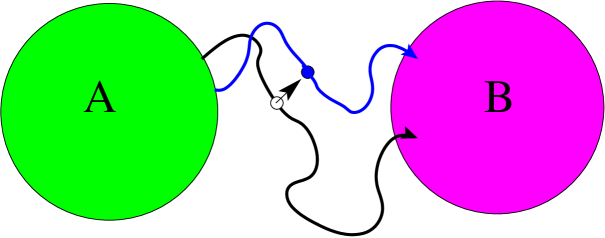
Figure 2: Illustration of the TPS shooting move using flexible path length. From an existing path (black line) a random timeslice is selected. Positions and/or velocities of this point are slightly modified giving a new phasepoint (blue dot). From this point, the equations of motion are integrated forward and backward in time until the trajectory hits $A$ or $B$.

Naturally, the random walk in path space should obey detailed balance

$$\frac{P_{\textrm{gen}}[{\bf x}^{\rm(o)}\rightarrow{\bf x}^{\rm(n)}]}{P_{\textrm{gen}}[{\bf x}^{\rm(n)}\rightarrow{\bf x}^{\rm(o)}]}\frac{P_{\textrm{acc}}[{\bf x}^{\rm(o)}\rightarrow{\bf x}^{\rm(n)}]}{P_{\textrm{acc}}[{\bf x}^{\rm(n)}\rightarrow{\bf x}^{\rm(o)}]}=\frac{P[{\bf x}^{\rm(n)}]}{P[{\bf x}^{\rm(o)}]},$$ (14)

where the superscripts (o) and (n) denote the old and new path respectively, and $P_{\rm gen}[{\bf x}\rightarrow{\bf x^{\prime}}]$ is the probability to generate path ${\bf x^{\prime}}$ staring from ${\bf x}$. Following the Metropolis-Hastings scheme, the acceptance rule of the whole shooting move can be written as

$$P_{\rm acc}[{\bf x}^{\rm(o)}\rightarrow{\bf x}^{\rm(n)}]=\hat{h}({\bf x}^{\rm(n)})\min\left[1,\frac{P[{\bf x}^{\rm(n)}]}{P[{\bf x}^{\rm(o)}]}\frac{P_{\rm gen}[{\bf x}^{\rm(n)}\rightarrow{\bf x}^{\rm(o)}]}{P_{\rm gen}[{\bf x}^{\rm(o)}\rightarrow{\bf x}^{\rm(n)}]}\right].$$ (15)

The generation probability is a product of different sub-probabilities. These are $P_{\rm sel}$, to select the shooting point, $P_{\rm ran}$, for the random modification of this shooting point, and $P_{\rm traj}$, which is the probability to obtain ${\bf x}^{(n)}$ by integrating the equations of motion backward and forward in time starting from the modified shooting point.

$$P_{\rm gen}[{\bf x}\rightarrow{\bf x^{\prime}}]=P_{\rm sel}(x_{\rm shoot}|{\bf x})\,P_{\rm ran}(x_{\rm shoot}\rightarrow x^{\prime}_{\rm shoot})\,P_{\rm traj}({\bf x^{\prime}}|x^{\prime}_{\rm shoot})$$ (16)

If we generate paths of a fixed length $n$ and if each timeslice has an equal probability to be selected then $P_{\rm sel}=1/n$. We come back to this point later on. In addition, TPS algorithms generally utilize a symmetric random modification of the shooting point: $P_{\rm ran}(x_{\rm shoot}\rightarrow x^{\prime}_{\rm shoot})=P_{\rm ran}(x^{\prime}_{\rm shoot}\rightarrow x_{\rm shoot})$. Therefore, both $P_{\rm sel}$ and $P_{\rm ran}$ cancel out in Eq. 15. The acceptance rule simplifies even further if we also assume that the dynamics obey the microscopic reversibility condition

$$\rho(x)p(x\rightarrow y)=\rho(y)p(\bar{y}\rightarrow\bar{x})$$ (17)

where $\bar{x}$ is the phasepoint $x$ with reversed velocities: $\bar{x}=(r,-v)$. This relation is very general and valid for a broad class of dynamics applying to both equilibrium and non-equilibrium systems [7]. By applying Eq. 17 several times on Eq. 13 we can show that

$$P[{\bf x}] = \rho(x_{j{\mathrm{d}}t})p(\bar{x}_{j{\mathrm{d}}t}\rightarrow\bar{x}_{(j-1){\mathrm{d}}t})p(\bar{x}_{(j-1){\mathrm{d}}t}\rightarrow\bar{x}_{(j-2){\mathrm{d}}t})\ldots p(\bar{x}_{{\mathrm{d}}t}\rightarrow\bar{x}_{0})$$ (18)

$$\times p(x_{j{\mathrm{d}}t}\rightarrow x_{(j+1){\mathrm{d}}t})p(x_{(j+1){\mathrm{d}}t}\rightarrow x_{(j+2){\mathrm{d}}t})\ldots p(x_{(n-1){\mathrm{d}}t}\rightarrow x_{n{\mathrm{d}}t})$$

is true for any timeslice $j$. For time-reversible dynamics the backward integration is simply obtained by reversing the velocities and integration forward in time. Hence, the generation probability $P_{\rm traj}({\bf x}|x_{\rm shoot})$ depends on exactly the same transition probabilities $p(x\rightarrow x^{\prime})$ and $p(\bar{x}\rightarrow\bar{x}^{\prime})$. This implies that all terms cancel out except the phasepoint density of the shooting point

$$P_{\rm acc}[{\bf x}^{\rm(o)}\rightarrow{\bf x}^{\rm(n)}]=\hat{h}({\bf x}^{\rm(n)})\min\left[1,\frac{\rho(x^{(n)}_{\rm shoot})}{\rho(x^{(o)}_{\rm shoot})}\right]$$ (19)

This is very convenient as this acceptance/rejection step can take place before the expensive trajectory generation takes place. Still, some (partly) completed trajectories will be rejected in the end due to the condition $\hat{h}({\bf x})$. However, as the new trajectory was generated from a small modification of an existing trajectory with $\hat{h}({\bf x})=1$ the chances are relatively high that the condition will be satisfied for the trial trajectory as well.

The sampling of trajectories under a given condition $\hat{h}$ might benefit from using a path ensemble that has a non-fixed length. Using a fixed path length to sample all possible trajectories between $A$ and $B$ is expensive as this length needs to be adapted to the longest pathway connecting these states. Many trajectories will reach $A$ to $B$ in a much shorter time and will, therefore, consist of unnecessary parts that are not relevant for the actual barrier crossing event. In addition, if trajectories have significant parts outside the barrier region, the shooting move becomes inefficient as many shooting points will lie inside the reactant or product well. Shooting from these points gives a very low probability to connect both states. Using flexible path lengths was first introduced in Ref. [8] within the context of the TIS rate evaluation. However, also for the generation of reactive trajectories, the flexible path ensemble is very useful and allows to generate paths that start and end just at the boundaries of $A$ and $B$ (see Fig. 2). The only difference with the previous example is that $P_{\rm sel}=1/n$ is not cancelled as the trajectory length can be different. Therefore, if the shooting procedure selects the timeslices by an equal probability, the acceptance rule becomes

$$P_{\rm acc}[{\bf x}^{\rm(o)}\rightarrow{\bf x}^{\rm(n)}]=\hat{h}({\bf x}^{\rm(n)})\min\left[1,\frac{\rho(x^{(n)}_{\rm shoot})}{\rho(x^{(o)}_{\rm shoot})}\frac{n^{(o)}}{n^{(n)}}\right]$$ (20)

with $n^{(o)},n^{(n)}$ the length of the old and new path. This expression is not so convenient as a rejection can only be made whenever the whole path is completed. Hence, the integration needs to be carried out even if $\rho(x^{(n)}_{\rm shoot})<<\rho(x^{(o)}_{\rm shoot})$ implying an almost certain rejection. We can, however, separate the acceptance into two steps by writing

$$P_{\rm acc}[{\bf x}^{\rm(o)}\rightarrow{\bf x}^{\rm(n)}]=\hat{h}({\bf x}^{\rm(n)})\min\left[1,\frac{\rho(x^{(n)}_{\rm shoot})}{\rho(x^{(o)}_{\rm shoot})}\right]\times\min\left[1,\frac{n^{(o)}}{n^{(n)}}\right]$$ (21)

This acceptance rule obeys detailed balance as well and allows to reject a modification of the shooting move that gives a too high energy. Still, even if the first step is accepted, the final trajectory might be rejected whenever it becomes too long compared to the previous path. We can improve the efficiency even further using following trick [8]. Instead of taking a random number $\alpha\in[0:1]$ after finishing our trajectory and then accept if $\alpha<n^{(o)}/n^{(n)}$, we will actually draw this random number before starting the integration of motions. As we now know that we will have to reject our trajectory whenever $\alpha<n^{(o)}/n^{(n)}$, we can simply define a maximum allowed path length of this trial move in advance

$$n^{\rm max}={\rm int}[n^{(o)}/\alpha]$$ (22)

This allows to directly stop our trial move whenever it exceeds this maximum path length.

The original TPS method also provided an algorithm to determine the reaction rate of the process. This approach has been improved by the TIS [8] and RETIS [9, 10] algorithms. Like RF, the TPS rate evaluation does require a RC (I will not make the distinction between orderparameter or RC). However, one can show that, compared to the RF method, the efficiency of TPS, TIS, and RETIS, is less sensitive to an improper choice of the RC [39].

The original TPS rate evaluation is based on following correlation function

$$C(t)=\frac{\left\langle h_{A}(x_{0})h_{B}(x_{t})\right\rangle}{\left\langle h_{A}(x_{0})\right\rangle}.$$ (23)

where $h_{A/B}(x)=1$ if $x\in A/B$ and 0 otherwise. Just like Eqs. 11, $C(t)$ will initially show some oscillations. However, if there is a separation of timescales, this correlation function grows linearly in time, $C(t)\sim k_{AB}t$, for times $\tau_{\rm mol}<t<\tau_{\rm rxn}$. Hence,

$$\tilde{k}_{AB}(t)=\frac{\mathrm{d}}{\mathrm{d}t}C(t)=\frac{\left\langle h_{A}(x_{0})\dot{h}_{B}(x_{t})\right\rangle}{\left\langle h_{A}(x_{0})\right\rangle},\quad k_{AB}=\tilde{k}_{AB}(t^{\prime})\textrm{ for }\tau_{\rm mol}<t<\tau_{\rm rxn}$$ (24)

The correlation function $C(t)$ is calculated in the TPS scheme using the shooting algorithm in combination with umbrella sampling. First, the fixed path length $t^{\prime}$ is fixed to a value where $C(t)$ should give a plateau. Then a series of path sampling simulations will be performed in which the final region $B$ is slowly shrunk in successive steps from the entire phase space to the final stable state $B$ [7]. For each step numerous trajectories are generated with that condition that the path should start in $A$ and end in the extended region $B$ at time $t^{\prime}$. The distribution of the path’s end-point will be binned into histograms that will be matched just like ordinary umbrella sampling. Once the fully matched histogram is obtained, $C(t)$ is obtained by integration of this histogram over the actual region $B$.

The approach is rather time-consuming because it can take a relatively long time $\tau_{\rm mol}$ before $C(t)$ reaches a plateau (longer than in a transmission coefficient calculation [7]). In Ref. [5] an improvement of this approach was presented in which the umbrella sampling series could be performed with paths shorter than $\tau_{\rm mol}$. The results were then corrected by a factor that is obtained from a single path sampling simulation using the longer paths. Unfortunately, the relative error in this correction factor is large if the path length is reduced too much, so that the gain in CPU efficiency remains limited [8]. Moreover, inspection of Eqs. (23) and (24) shows that a necessary cancellation of positive and negative terms can slow down the convergence of the MC sampling procedure.

4 Transition Interface Sampling

TIS is a more efficient way to calculate reaction constant than the method discussed above. The TIS methodology is also the basis of several other algorithms [11, 13, 9, 44, 45] of which the PPTIS, RETIS, and FFS methods will be discussed in forth-coming sections. The TIS rate equation is related to both the EPF expression, Eq. 9, and to the correlation function used in TPS, Eq. 23, albeit using different kind of characteristic functions. Instead of using the characteristic functions of the stable states $A$ and $B$, we will redefine the correlation function using overall states $\mathcal{A}$ and $\mathcal{B}$. These states do not only depend on the position at the time of consideration but also on its past behavior. Overall state $\mathcal{A}$ covers all phase space points lying inside stable region $A$, which constitutes the largest part, but also all phase space points that visit $A$, before reaching $B$ when the equations of motion are integrated backward in time. In other words, all phasepoints that were more recently in $A$ rather than in $B$. Similarly, state $\mathcal{B}$ comprises stable state B and all phase points, coming directly from this state in the past, i.e. with- out having been in $A$. The corresponding correlation function is

$$C(t)=\frac{\left\langle h_{\mathcal{A}}(x_{0})h_{\mathcal{B}}(x_{t})\right\rangle}{\left\langle h_{\mathcal{A}}(x_{0})\right\rangle}.$$ (25)

where $h_{\mathcal{A}}(x_{0})=h^{b}_{AB}(x_{0})$ and $h_{\mathcal{B}}(x_{0})=h^{b}_{BA}(x_{0})$. Contrary to Eq. 23, this correlation function has no oscillatory behavior during a molecular timescale $\tau_{\rm mol}$. On the contrary, it exhibits a linear regime $\sim k_{AB}t$ for $0<t<\tau_{\rm rxn}$. The system will only transfer from overall state $\mathcal{A}$ to overall state $\mathcal{B}$ when it enters region $B$ for the first time since it left region $A$. If it leaves state $B$ shortly thereafter, it will remain in $\mathcal{B}$. Therefore $h_{\mathcal{B}}(x_{t})$ and $h_{\mathcal{A}}(x_{t})$ do not show the fast fluctuations that are found for $h_{B}(x_{t})$ and $h_{A}(x_{t})$. As Eq. 25 is linear from the start, we can simply take the time derivative at $t=0$, which gives

$$k_{AB} = \frac{\left\langle h_{\mathcal{A}}(x_{0})\dot{h}_{\mathcal{B}}(x_{0})\right\rangle}{\left\langle h_{\mathcal{A}}(x_{0})\right\rangle}=\lim_{{\mathrm{d}}t\rightarrow 0}\frac{1}{{\mathrm{d}}t}\frac{\left\langle h^{b}_{AB}(x_{0})\theta(\lambda_{B}-\lambda(x_{0}))\theta(\lambda(x_{{\mathrm{d}}t})-\lambda_{B})\right\rangle}{\left\langle h_{\mathcal{A}}(x_{0})\right\rangle}$$ (26)

$$= \frac{\left\langle h^{b}_{AB}(x_{0})\dot{\lambda}\left(x_{0}\right)\delta(\lambda(x_{0})-\lambda_{B})\theta\left(\dot{\lambda}\left(x_{0}\right)\right)\right\rangle}{\left\langle h_{\mathcal{A}}(x_{0})\right\rangle}$$

The resulting expression is basically the EPF expression (Eq. 9) through the interface $\lambda_{B}$. At a first sight it might seem that generating long trajectories is no longer needed. As we only need ${\mathrm{d}}C(t)/{\mathrm{d}}t$ at $t=0$, the minimum time range over which we need to calculate $C(t)$ is $[0:{\mathrm{d}}t]$ instead of $[0:\tau_{\rm mol}]$. Unfortunately, unlike $h_{A}(x_{0})$ and $h_{B}(x_{0})$, the determination of $h_{\mathcal{A}}(x_{0})$ and $h_{\mathcal{B}}(x_{0})$ can not be done instantaneously. For this we still need to integrate the equations of motion. However, for most $x_{0}$, $h_{\mathcal{A}}(x_{0})$/$h_{\mathcal{B}}(x_{0})$ can be assigned 1 or 0 using a much shorter backward trajectory than $\tau_{\rm mol}$. For stochastic dynamics $h_{\mathcal{A}}(x_{0})$/$h_{\mathcal{B}}(x_{0})$ can be, strictly speaking, a fractional number. However, there is generally no need to know this fractional number for a specific phasepoint, except for committor analysis [46, 47, 48, 49, 14]. Hence, TIS algorithms will generally compute $h_{A}(x_{0})$/$h_{B}(x_{0})$ for one specific path to which $x_{0}$ belongs. Conceptually, it is therefore more accurate to speak of a MC sampling in pathspace rather than phasespace. The TIS correlation function has an additional advantage that the reaction rate is somewhat better defined if the separation of timescales $\tau_{\rm mol}\ll\tau_{\rm rxn}$ is not sufficiently obeyed. The fact that the derivative of $C(t)$ is taken at $t=0$ makes corrections like the one suggested in Ref. [50] unnecessary.

The TIS algorithm expresses the rate equation, Eq. 26, as a product of different terms. Each term has a much higher value than the final rate and is, therefore, much easier to compute. To introduce the TIS and PPTIS expression, that I will discuss in the next section, it is convenient to introduce following crossing probabilities that depend on four non-intersecting interfaces $\{x|\lambda(x)=\lambda_{i}\},\{x|\lambda(x)=\lambda_{j}\},\{x|\lambda(x)=\lambda_{k}\},\{x|\lambda(x)=\lambda_{l}\}$

$$P(^{k}_{l}|_{i}^{j}) = \lim_{{\mathrm{d}}t\rightarrow 0}\frac{\langle h^{b}_{ij}(x_{0})\theta(\lambda_{j}-\lambda(x_{0}))\theta(\lambda(x_{{\mathrm{d}}t})-\lambda_{j})h^{f}_{kl}(x_{0})\rangle}{\langle h^{b}_{ij}(x_{0})\theta(\lambda_{j}-\lambda(x_{0}))\theta(\lambda(x_{{\mathrm{d}}t})-\lambda_{j})\rangle}$$ (27)

$$= \frac{\langle h^{b}_{ij}(x_{0})\dot{\lambda}\left(x_{0}\right)\delta\left(\lambda\left(x_{0}\right)-\lambda_{j}\right)\theta\left(\dot{\lambda}\left(x_{0}\right)\right)h^{f}_{kl}(x_{0})\rangle}{\langle h^{b}_{ij}(x_{0})\dot{\lambda}\left(x_{0}\right)\delta\left(\lambda\left(x_{0}\right)-\lambda_{j}\right)\theta\left(\dot{\lambda}\left(x_{0}\right)\right)\rangle}\textrm{ for }\lambda_{j}>\lambda_{i}$$

For $\lambda_{j}<\lambda_{i}$ we simply need to replace $\theta(\lambda_{j}-\lambda(x_{0}))\theta(\lambda(x_{{\mathrm{d}}t})-\lambda_{j})$ by $\theta(\lambda(x_{0})-\lambda_{j})\theta(\lambda_{j}-\lambda(x_{{\mathrm{d}}t}))$ in the first line or $\dot{\lambda}\left(x_{0}\right)\delta\left(\lambda\left(x_{0}\right)-\lambda_{j}\right)\theta\left(\dot{\lambda}\left(x_{0}\right)\right)$ by $-\dot{\lambda}\left(x_{0}\right)\delta\left(\lambda\left(x_{0}\right)-\lambda_{j}\right)\theta\left(-\dot{\lambda}\left(x_{0}\right)\right)$ in the second line of the above definition. Eq. 27 defines a conditional crossing probability. It is the probability that the system will cross interface $\lambda_{k}$ before $\lambda_{l}$ under a twofold condition. These conditions are that the system should cross interface $\lambda_{j}$ right now at time $t=0$, while $\lambda_{i}$ was more recently crossed than $\lambda_{j}$ in the past.

Using these crossing probabilities, one can prove that Eq. 26 is equivalent to the product of the initial flux times the overall crossing probability [8]

$$k_{AB}=\frac{\langle\dot{\lambda}\left(x_{0}\right)\delta\left(\lambda\left(x_{0}\right)-\lambda_{0}\right)\theta\left(\dot{\lambda}\left(x_{0}\right)\right)\rangle}{\langle h_{\mathcal{A}}(x_{0})\rangle}\times P(^{n}_{0}|^{0}_{0^{-}})\equiv f_{A}{\mathcal{P}}_{A}(\lambda_{n}|\lambda_{0})$$ (28)

where $\lambda_{0}$ and $\lambda_{n}$ are the boundaries of the stable states $A$ and $B$. $f_{A}$ is just the flux out of state $A$ that can be computed with standard MD as the boundary of $A$ is set at the left side of the barrier region. The minus in $0^{-}$ is to denote an interface $\lambda_{0}-\epsilon$ which is put there to indicate the direction of the crossing at $t=0$. The overall crossing probability ${\mathcal{P}}_{A}(\lambda_{n}|\lambda_{0})=P(^{n}_{0}|^{0}_{0^{-}})$ is the probability that once $\lambda_{0}$ is crossed, $\lambda_{n}$ will be crossed before a recrossing with $\lambda_{0}$ occurs. This probability is very small, but it can be calculated by defining $n-1$ non-intersecting interfaces in between $\lambda_{0}$ and $\lambda_{n}$ and express the overall crossing probability as the following product [8]

$${\mathcal{P}}_{A}(\lambda_{n}|\lambda_{0})=\prod_{i=0}^{n-1}{\mathcal{P}}_{A}(\lambda_{i+1}|\lambda_{i})$$ (29)

The factorization of ${\mathcal{P}}_{A}(\lambda_{n}|\lambda_{0})$ into probabilities ${\mathcal{P}}_{A}(\lambda_{i+1}|\lambda_{i})$ that are much higher than the overall crossing probability, is the basis of the importance sampling approach. It is important to note that ${\mathcal{P}}_{A}(\lambda_{i+1}|\lambda_{i})$ are in fact complicated history dependent conditional probabilities. If we consider all possible pathways that start at $\lambda_{A}$ and end by either crossing $\lambda_{A}$ or $\lambda_{B}$, while have at least one crossing with $\lambda_{i}$ in between, the fraction that crosses $\lambda_{i+1}$ as well equals ${\mathcal{P}}_{A}(\lambda_{i+1}|\lambda_{i})$. This basically reduces the problem to a correct sampling of trajectories that should obey the $\lambda_{i}$ crossing condition (See fig. 3). From now on we will call this the $[i^{+}]$ path ensemble. In TIS, this is done via the shooting algorithm for flexible path lengths as is discussed in previous section (For a full flowchart diagram of the TIS algorithm see Ref. [51]).

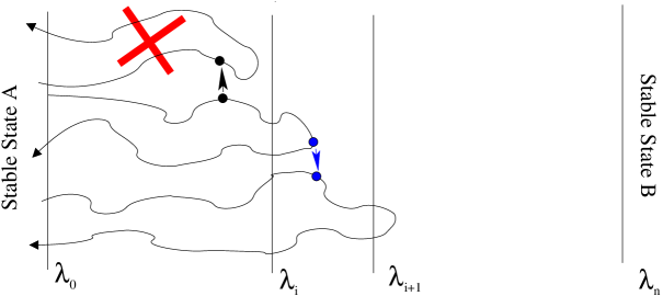
Figure 3: The TIS path ensemble $[i^{+}]$ is required to calculate the conditional crossing probability ${\mathcal{P}}_{A}(\lambda_{i+1}|\lambda_{i})$. For this purpose we apply the shooting move to generate all possible trajectories starting at $\lambda_{0}$ and ending at $\lambda_{0}$ or $\lambda_{n}$ with at least one crossing with $\lambda_{i}$. Suppose the algorithm starts with the middle path that already fulfills these requirements. A shooting point is randomly selected and modified (black dots). However, the trajectory that starts out from this point (top trajectory) fails to cross $\lambda_{i}$ and is therefore rejected and the old path is counted again. A new shooting (blue dots) generates a valid trajectory that not only crosses $\lambda_{i}$ but $\lambda_{i+1}$ as well. This trajectory is called ”successful”. The fraction of successful trajectories in this ensemble determine ${\mathcal{P}}_{A}(\lambda_{i+1}|\lambda_{i})$.

The number of interfaces and their separation should be set to maximize efficiency. In Ref. [40, 39] it was found that the optimal interface separation is obtained when one out of five trajectories reach the next interface. In addition, one can define a set of sub-interfaces of arbitrary separation in order to construct the crossing probability as a continuous function. This strictly decreasing function could be viewed as the dynamical analogue of the free energy profile $F(\lambda)$.

There are some small differences how to treat the path ensemble $[i^{+}]$ regarding the end-point of the path. In the first TIS algorithms, the trajectory could reach upto $\lambda_{i+1}$ where the trajectory was stopped and assigned successful. More recent simulations continue the trajectory until reaching the stable states $A$ or $B$ each time. The additional cost is very limited as about 80% is not reaching $\lambda_{i+1}$ and need to be followed until reaching $A$ anyway. The choice to continue the trajectory even after $\lambda_{i+1}$ has the advantage that one can start the $[i^{+}]$ path ensemble without the need to fix a value for $\lambda_{i+1}$ beforehand. After some simulation cycles the $\lambda_{i+1}$ can be set to have the optimal 20% success-rate after which one can start the $[(i+1)^{+}]$ path ensemble. In addition, the new approach makes it much more easy to use replica exchange which we will discuss in Sec. 7.

The simplicity of Eq. 29 is deceptive and could be mistaken as a Markovian approximation. The reason that the equation is still exact lies in the fact that the crossing probabilities are history dependent and by the fact that it only considers first crossing events. We can argue the exactness of the equations also in another way. Suppose we want to calculate the probability to go from $\lambda_{0}$ to $\lambda_{1}$ to $\lambda_{2}$ …to $\lambda_{n}$ in successive jumps. This probability can be expressed as

$$P(\lambda_{0}\rightarrow\lambda_{1}\rightarrow\lambda_{2}\rightarrow\ldots\rightarrow\lambda_{n}) = P(\lambda_{0})\times P(\lambda_{0}\rightarrow\lambda_{1}|\lambda_{0})\times P(\lambda_{1}\rightarrow\lambda_{2}|\lambda_{0}\rightarrow\lambda_{1})$$ (30)

$$\times P(\lambda_{2}\rightarrow\lambda_{3}|\lambda_{0}\rightarrow\lambda_{1}\rightarrow\lambda_{2})\times\ldots$$

$$\times P(\lambda_{n-1}\rightarrow\lambda_{n}|\lambda_{0}\rightarrow\lambda_{1}\rightarrow\lambda_{2}\rightarrow\ldots\lambda_{n-2}\rightarrow\lambda_{n-1})$$

This is an exact non-Markovian expression for this specific crossing sequence that looks similar to Eq. 29. However, it doesnot say anything about the many different trajectories that could connect $\lambda_{0}$ with $\lambda_{n}$. For instance, we should also take into account the sequence $\lambda_{0}\rightarrow\lambda_{1}\rightarrow\lambda_{2}\rightarrow\lambda_{1}\rightarrow\lambda_{2}\rightarrow\lambda_{3}\rightarrow\ldots\lambda_{n-1}\rightarrow\lambda_{n}$. Therefore, it might seem that the right expression should look much more complicated than Eq. 29. The trick, however, is that this last sequence can not occur if we only consider first crossing events. When we move back to $\lambda_{1}$ in the third step, this move will simply not considered as it is a second visit since leaving $\lambda_{0}$. Hence, the successive sequence $\lambda_{0}\rightarrow\lambda_{2}\rightarrow\lambda_{3}\rightarrow\ldots\lambda_{n-1}\rightarrow\lambda_{n}$ is the only possible sequence of first crossing events that brings you from $\lambda_{0}$ to $\lambda_{n}$.

5 Partial Path Sampling

The PPTIS is a variation of the TIS algorithm that was devised to treat diffusive barrier crossings [11]. Despite the existence of a fine separation of timescale, i.e. the time to cross the barrier is still negligible compared to the time spend in the reactant well, the path length can become too long for an effective computation of the reaction rate. This is the case if the barriers are sufficiently high to ensure exponential relaxation, but not very sharp so that system can move backward and forward on the barrier before it eventually drops off. The PPTIS equation depends on the same rate equation as TIS

$$k_{AB}=f_{A}P(^{n}_{0}|^{1}_{0})$$ (31)

The only difference with Eq. 28 is that we now consider the condition $|^{1}_{0})$ instead of $|^{0}_{0^{-}})$, but this is just a technical detail. If we take $\lambda_{1}=\lambda_{0}+\epsilon$ the equations become equivalent. However, $\lambda_{1}$ can be any value that is somewhat larger than $\lambda_{0}$ by redefining $f_{A}$ as the effective flux through $\lambda_{1}$. This implies that we should count the positive crossings with $\lambda_{1}$ whenever the system leaves the stable state $A:\{x|\lambda(x)<\lambda_{0}\}$. However, the next positive crossing should only be counted if the system has revisited $A$ again. The PPTIS approach tries to avoid the generation of very long trajectories using a soft Markovian approximation. The PPTIS scheme assumes that for a well positioned set of interfaces the system will lose its memory over a distance that is similar to the interface separation. This implies for any $m>1$

$$P(^{l}_{k}|^{j}_{j\pm m})\approx P(^{l}_{k}|^{j}_{j\pm 1})$$ (32)

The PPTIS algorithm consist again of a series of path sampling simulations. Each PPTIS simulation samples a certain path ensemble in which trajectories are confined within two next-nearest interfaces. For instance, the $[i^{\pm}]$ path ensemble will consist of all possible trajectories starting and ending at either $\lambda_{i+1}$ or $\lambda_{i-1}$ having at least one crossing with the middle interface $\lambda_{i}$. From these simulations the following short-distance crossing can be obtained

$$p_{i}^{\pm}\equiv P(^{i+1}_{i-1}|_{i-1}^{i}),\quad p_{i}^{=}\equiv P(^{i-1}_{i+1}|_{i-1}^{i}),\quad p_{i}^{\mp}\equiv P(^{i-1}_{i+1}|_{i+1}^{i}),\quad p_{i}^{\ddagger}\equiv P(^{i+1}_{i-1}|_{i+1}^{i})$$ (33)

with $p_{i}^{\pm}+p_{i}^{=}=p_{i}^{\mp}+p_{i}^{\ddagger}=1$. For instance, $p_{i}^{\pm}$ is determined by dividing the number of trajectories in the $[i^{\pm}]$ ensemble that start at $\lambda_{i-1}$ and end at $\lambda_{i+1}$ divided by all trajectories that start at $\lambda_{i-1}$.

Once these short distance crossing probabilities are obtained with sufficient accuracy, the overall crossing probability can be obtained. One way to do this is to use these probabilities as input for a kinetic MC simulation [52]. However, this is not needed for a one-dimensional RC which allows an elegant analytical treatment [11]. Naturally, $P(^{2}_{0}|^{1}_{0})=p_{1}^{\pm}$, but the calculation of $P(^{3}_{0}|^{1}_{0})$ requires already to sum up the trajectories $0\rightarrow 1\rightarrow 2\rightarrow 3$, $0\rightarrow 1\rightarrow 2\rightarrow 1\rightarrow 2\rightarrow 3$, etc. However, as shown in Ref. [11], one can derive following recursive relations to make this infinite summation of all trajectories (include the ones of infinite length!). These PPTIS recursive relations are the following

$$P(^{m+1}_{0}|^{1}_{0}) = \frac{p_{m}^{\pm}P(^{m}_{0}|^{1}_{0})}{p_{m}^{\pm}+p_{m}^{=}P(^{0}_{m}|^{m-1}_{m})},\quad P(^{0}_{m+1}|^{m}_{m+1})=\frac{p_{m}^{\mp}P(^{0}_{m}|^{m-1}_{m})}{p_{m}^{\pm}+p_{m}^{=}P(^{0}_{m}|^{m-1}_{m})}$$ (34)

or, by defining the long-distance crossing probabilities $P^{+}_{m}\equiv P(^{m}_{0}|^{1}_{0}),P_{m}^{-}=P(^{0}_{m}|^{m-1}_{m})$

$$k_{AB} = f_{A}P^{+}_{n}$$

$$P_{m+1}^{+} = \frac{p_{m}^{\pm}P^{+}_{m}}{p_{m}^{\pm}+p_{m}^{=}P_{m}^{-}},\quad P^{-}_{m+1}=\frac{p_{m}^{\mp}P^{-}_{m}}{p_{m}^{\pm}+p_{m}^{=}P^{-}_{m}},\quad\textrm{for }m>1,\quad P^{+}_{1}=P^{-}_{1}=1$$ (35)

Hence, starting from the initial conditions for $(P^{+}_{1},P^{-}_{1})=(1,1)$, one can successively solve $(P^{+}_{2},P^{-}_{2}),(P^{+}_{3},P^{-}_{3}),\ldots,(P^{+}_{n},P^{-}_{n})$ via Eq. 35. It is important to note that $P^{-}_{j}$ is not exactly the same as $P^{+}_{j}$ in the reverse direction. Only for $j=n$ these two probabilities can be viewed as mirror images.

Here, I will derive an alternative recursive relation that does not require the auxiliary reverse probabilities $P^{-}_{j}$. The derivation is similar to the one presented in the supplemental information of Ref. [53] which treats the simpler hopping process. To achieve this, we will bring $P(^{0}_{m}|^{m-1}_{m})$ in front of Eq. 34.

$$P(^{0}_{m}|^{m-1}_{m}) =\frac{p_{m}^{\pm}\left[P(^{m}_{0}|^{1}_{0})-P(^{m+1}_{0}|^{1}_{0})\right]}{p_{m}^{=}P(^{m}_{0}|^{1}_{0})}$$ (36)

or by incrementing $m$

$$P(^{0}_{m+1}|^{m}_{m+1}) =\frac{p_{m+1}^{\pm}\left[P(^{m+1}_{0}|^{1}_{0})-P(^{m+2}_{0}|^{1}_{0})\right]}{p_{m+1}^{=}P(^{m+2}_{0}|^{1}_{0})}$$ (37)

Moreover, we can write for $P(^{m+1}_{0}|^{1}_{0})$

$$P(^{m+1}_{0}|^{1}_{0}) = P(^{m}_{0}|^{1}_{0})P(^{m+1}_{0}|^{m}_{m-1})$$ (38)

$$= P(^{m}_{0}|^{1}_{0})\left(1-P(^{0}_{m+1}|^{m}_{m-1})\right)$$

$$= P(^{m}_{0}|^{1}_{0})\left(1-P(^{0}_{m+1}|^{m}_{m+1})p_{m}^{=}/p_{m}^{\mp}\right)$$

Then, we substitute Eq. 37 in Eq. 38 and bring $P(^{m+2}_{0}|^{1}_{0})$ in front which yields

$$P(^{m+2}_{0}|^{1}_{0}) =\frac{p_{m}^{=}p_{m+1}^{\pm}P(^{m}_{0}|^{1}_{0})P(^{m+1}_{0}|^{1}_{0})}{\left(p_{m}^{\mp}p_{m+1}^{=}+p_{m}^{=}p_{m+1}^{\pm}\right)P(^{m}_{0}|^{1}_{0})-p_{m}^{\mp}p_{m+1}^{=}P(^{m+1}_{0}|^{1}_{0})}$$ (39)

or

$$k_{AB} = f_{A}P^{+}_{n}$$

$$P_{m+2}^{+} = \frac{p_{m}^{=}p_{m+1}^{\pm}P_{m}^{+}P_{m+1}^{+}}{\left(p_{m}^{\mp}p_{m+1}^{=}+p_{m}^{=}p_{m+1}^{\pm}\right)P_{m}^{+}-p_{m}^{\mp}p_{m+1}^{=}P_{m+1}^{+}},\quad P_{1}^{+}=1,\quad P_{2}^{+}=p_{1}^{\pm}$$ (40)

In the case of a full Markovian assumption, $p_{i}^{\pm}=p_{i}^{\ddagger}$ and $p_{i}^{\mp}=p_{i}^{=}$, we reobtain the simpler expression of Ref. [53]. For some this new expression might seem more esthetic as the set of two equations has now been transferred into a single recursive equation without relying on the auxiliary probability $P^{-}_{m}$. The new function has its utility [53], but is numerically somewhat problematic as it can sometimes produce zeros in both nominator and denominator that cancel, but is not practical for numerical calculations.

The positioning of interfaces is crucial in PPTIS. On one hand, one would like to put them close together to improve efficiency. On the other hand, putting them to close will introduce systematic errors due to a decrease of history dependence of the hopping probabilities, which invalidates Eq. 32. A way to measure whether the interfaces are sufficiently far is the calculation of a memory-loss function [11]. However, the memory-loss function can only provide a necessary but not necessarily sufficient condition for this separation. In fig. 4 we give two examples of well and badly placed interfaces.

The milestoning method [12] is very similar to PPTIS. There are basically two important differences. Milestoning assumes full memory loss once the system hits an interface. In our notation this could be rephrased as $P(^{l}_{k}|^{j}_{j\pm m})\approx P(^{l}_{k}|^{j}_{j})$. This is a stronger approximation than Eq. 32. The approximation of milestoning becomes exact, if the interfaces coincide with the iso-committor functions [54], but these are difficult determine. On the other hand, milestoning is more precise in the construction of the time-evolution of the system by making the crossing probabilities time-dependent. This is important if there is not a clear separation of timescales and also allows to calculate other dynamical properties like diffusion. Hence, instead of $p_{i}^{\pm},p_{i}^{=},p_{i}^{\mp},p_{i}^{\ddagger}$ with $p_{i}^{\pm}+p_{i}^{=}=p_{i}^{\mp}+p_{i}^{\ddagger}=1$, milestoning calculates for each interface the time-dependent probability densities $p_{i}^{+}(t),p_{i}^{-}(t)$ with $\int_{0}^{\infty}[p_{i}^{+}(t)+p_{i}^{-}(t)]{\mathrm{d}}t=1$. The strengths of PPTIS and milestoning do not exclude each other and could be unified into a single method as was suggested in Ref. [55]. A realization of such a method was recently published [56].

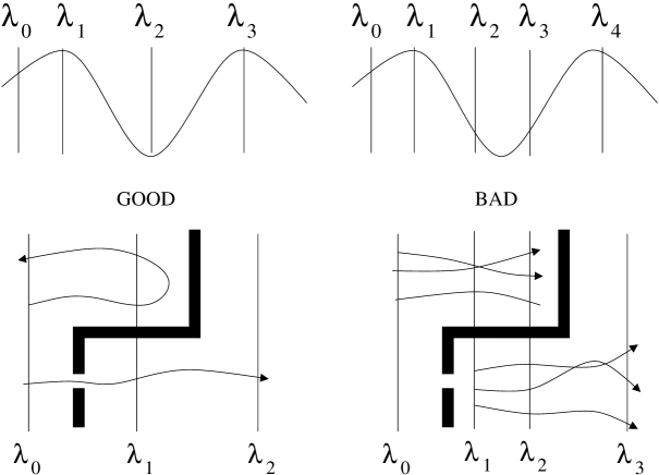
Figure 4: Examples of well and badly positioned interfaces with respect to the memory-loss assumption Eq. 32. The top situation requires a good description of the kinetic correlations whenever the top of the barrier has many small local wells. At the left, the interfaces are correctly placed. Once the system crosses $\lambda_{1}$ it will gain a lot of kinetic energy when arriving at $\lambda_{2}$. Henceforth, the chances are high that the system won’t get trapped and directly moves upward to cross $\lambda_{3}$. The PPTIS simulation for this interface configuration will show that $p_{2}^{\pm}\gg\frac{1}{2}$ as it should. At the right-hand side we have put an additional interface inside the local well. The $[3^{\pm}]$ path ensemble will consists of trajectories having a much lower kinetic energy than the $[2^{\pm}]$ ensemble of the left-hand side. Henceforth, the right-hand side will overestimate the probability to get trapped. The bottom picture shows impermeable wall (thick black line) with a small hole. The left hand side shows a correct positioning of interfaces. The pathways that are generated from $\lambda_{0}$ to $\lambda_{2}$ all have to move through the small hole. Conversely, the right-hand side shows a bad overlap between the $[1^{\pm}]$ and $[2^{\pm}]$ path ensembles which might give the impression that trajectories can tunnel through the wall.

6 Forward Flux Sampling

FFS was originally developed for the special case of biochemical networks that do not obey equilibrium statistics nor time-reversibility [13]. However, its advantageous implementation and apparent efficiency has gained this method a fast increasing popularity for equilibrium systems as well. FFS is based on the same theoretical TIS rate equation 26. However, the fundamental difference is the sampling move. While the principal sampling move in TIS is the shooting move, FFS is based on a non-Metropolis MC scheme called splitting [57, 58]. This approach requires stochastic dynamics, although it has been suggested that FFS is able to treat deterministic dynamics utilizing the Lyapunov instability [59, 60] using small ’invisible’ stochastic noises [61]. Like TIS, FFS consists of a straightforward MD simulation, from which the escape flux $f_{A}$ is obtained, followed by a series of path sampling simulations. However, besides giving the flux value, the MD simulation also provides the starting conditions for the path sampling simulations. Each time that the first interface $\lambda_{0}$ is crossed in the positive direction, this phasepoint just after the interface is stored on the hard-disk. In the first path simulation, performing the $[0^{+}]$ path ensemble, these points are used as starting points for the trajectories that are continued until reaching $\lambda_{1}$ or returning to $\lambda_{0}$. Naturally, stochasticity is of eminent importance, otherwise all these trajectories would just reproduce parts of MD simulation. The endpoints of the trajectories that successfully reach $\lambda_{1}$ are stored again and serve as initial points for the $[1^{+}]$ ensemble. The path ensembles are executed one after the other by the same procedure until reaching state $B$ (See fig. 5).

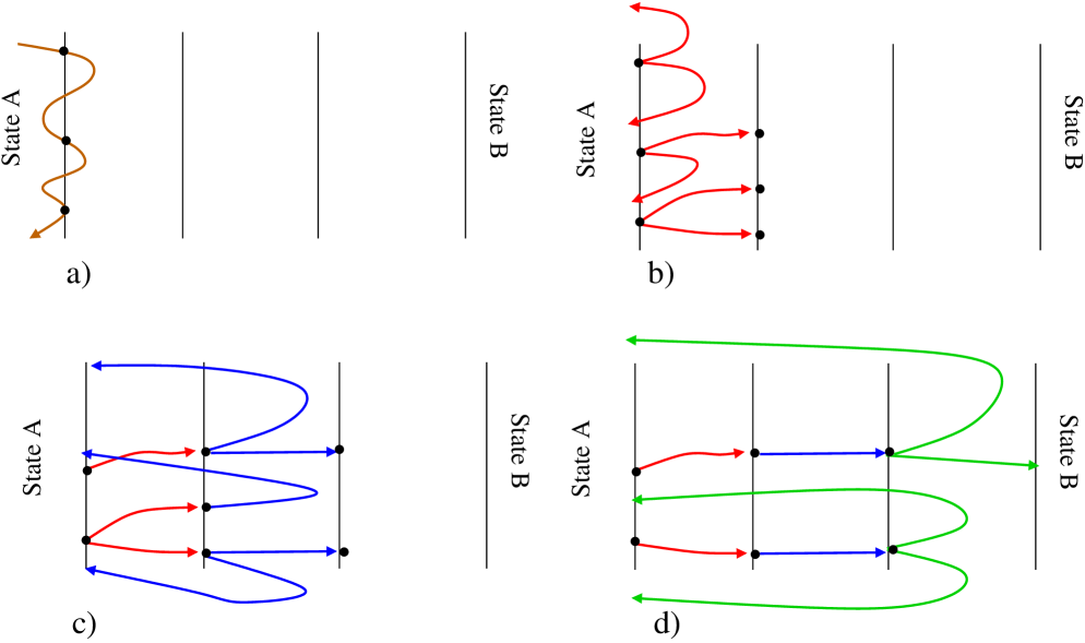
Figure 5: Illustration of FFS algorithm. a) shows the initial MD simulation that is needed to calculate the flux $f_{A}$. The positive crossing points (black dots) are stored. b) Starting from the stored MD crossing points a number of trajectories are released. The endpoints of the successful trajectories (that reach $\lambda_{1}$) are stored again and used for the next path ensemble simulation c). Finally, the reactant state will be reached d).

There are advantages and disadvantages compared to the TIS algorithm. The most important advantage of FFS is that it allows to treat non-equilibrium systems as it does not require any knowledge about the phasepoint density. TIS employs the shooting move that requires to know $\rho(x)$ for the acceptance, Eq. 19. In addition, FFS does not require any integration of motion backward in time. Therefore, time-reversibility is not required. Moreover, unlike PPTIS, FFS is, in principle, equally exact as TIS. However, if one has to chose between TIS and FFS for equilibrium dynamics, one has to consider following points. FFS will generally create more trajectories for the same number of MD steps as it recycles previously generated trajectories. Moreover, there are no rejections like there are in TIS and any other Metropolis based MC scheme. In practice, the reduction in MD steps will be limited to a certain factor ($\approx 2,3$) as the unsuccessful trajectories, which is the largest part, have to be followed until reaching state $A$. On the other hand, the FFS trajectories will be much more correlated than the TIS trajectories. This implies that FFS needs much more trajectories than TIS to obtain the same accuracy. One reason for this, is that FFS generates several trajectories having the same starting point. Absence of stochasticity will result that all these trajectories basically coincide. Fully Brownian motion does not exclude correlation effects either as the successful trajectories starting from the same point will hit the next interface in a confined region. The size of this region is determined by the diffusion orthogonal to the RC and the time it takes to go from interface to the other. Besides correlations within a certain path ensemble, the FFS method also introduces correlations between the different ensembles. This is a crucial difference with TIS where the MD simulation and all path simulations are independent. One of its consequences is that the FFS is more sensitive to the RC than TIS or even RF [39]. An efficiency analysis of FFS [62] ignores this correlation effect. This can be a rather crude approximation that is probably only valid when interfaces are approximately equal to the isocommittor surfaces. Suppose $\lambda^{\perp}$ denotes a coordinate orthogonal to the RC. Let ${\mathcal{P}}_{A}(\lambda_{n}|\lambda_{0};\lambda^{\perp})$ be the overall crossing probability from $\lambda_{0}$ to $\lambda_{n}$ starting from a point $\lambda^{\perp}$ on the first interface. Then, the full overall crossing probability is given by

$${\mathcal{P}}_{A}(\lambda_{n}|\lambda_{0})=\int{\mathrm{d}}\lambda^{\perp}\,{\mathcal{P}}_{A}(\lambda_{n}|\lambda_{0};\lambda^{\perp})\rho(\lambda^{\perp}|\lambda_{0})$$ (41)

where $\rho(\lambda^{\perp}|\lambda_{0})$ is the probability density of $\lambda^{\perp}$ on interface $\lambda_{0}$. FFS will suffer considerably when the distributions $\rho(\lambda^{\perp}|\lambda_{0})$ and ${\mathcal{P}}_{A}(\lambda_{n}|\lambda_{0};\lambda^{\perp})$ are not overlapping. In that case, FFS will miss important crossing points that are significant for the rate evaluation. Some studies have shown that FFS can significantly underestimate reaction rates [63, 64] in practical cases. Sampling artefacts like this, are also not yet fully excluded as possible explanation for some surprising results on non-equilibrium nucleation [65].

This issue will be most sensitive to the MD and the first interface ensembles on which all the further results will depend. If $\lambda_{1},\lambda_{2},\ldots,\lambda_{n-1}$ are isocommittor surfaces then ${\mathcal{P}}_{A}(\lambda_{n}|\lambda_{i};\lambda^{\perp})$ is a constant as function of $\lambda^{\perp}$ which eliminates the problem. This is the reason that Borrero et al. devised a FFS scheme in which the interfaces are repositioned on-the-fly in order to obtain a proper RC [66].

TIS has the advantage that it can relax the history of the path via the backward integration. Therefore, the distribution density $\rho(\lambda^{\perp}|\lambda_{0})$ can change when considering the different path ensembles. TIS can give correct results even if the sampled distribution of starting points $\lambda^{\perp}$ of the final $[n-1^{+}]$ trajectories do not overlap with the initial MD crossing points [67].

7 Replica-Exchange TIS

In Ref. [9], I showed that a special type of replica exchange [68, 69] can significantly improve the TIS efficiency (See also Ref [10] for some extensions of this approach). A crucial difference with standard RE, which has also been applied to TPS [70], is that the RETIS method does not require additional simulations at elevated temperatures. Instead, swaps are attempted between the different TIS path ensembles. For this purpose, RETIS has replaced the initial MD simulation by another path ensemble, called $[0^{-}]$, that consists of all path that start at $\lambda_{0}=\lambda_{A}$, then go in the opposite direction away from the barrier inside state $A$, and finally end at $\lambda_{0}$ again. The flux is then obtained from the average path length of the $[0^{-}]$ and $[0^{+}]$ ensembles as follows [9].

$$f_{A}=\Big{(}\langle t_{\rm path}^{[0^{-}]}\rangle+\langle t_{\rm path}^{[0^{+}]}\rangle\Big{)}^{-1}$$ (42)

where $\langle t_{\rm path}^{[0^{-}]}\rangle,\langle t_{\rm path}^{[0^{+}]}\rangle$ are the average path lengths in the $[0^{-}]$ and $[0^{+}]$ path ensembles respectively.

As the dynamical process is now fully described by path simulations with different interface-crossing conditions, the exchange of trajectories between them becomes extremely efficient, especially if the process possesses multiple reaction channels [67]. The methodology avoids the need of doing additional simulations at elevated temperatures and even gives paths for free as for most swapping moves whole trajectories are being swapped. Only when a swapping between the $[0^{-}]$ and $[0^{+}]$ ensembles are attempted, two phase points are interchanged. From the last point of the $[0^{-}]$ trajectory a new path in the $[0^{+}]$ is generated. Reversely, the first point of the old $[0^{+}]$ path will serve to generate a new path in the $[0^{-}]$ ensemble by integrating the equations of motion backward in time (See Fig. 6).

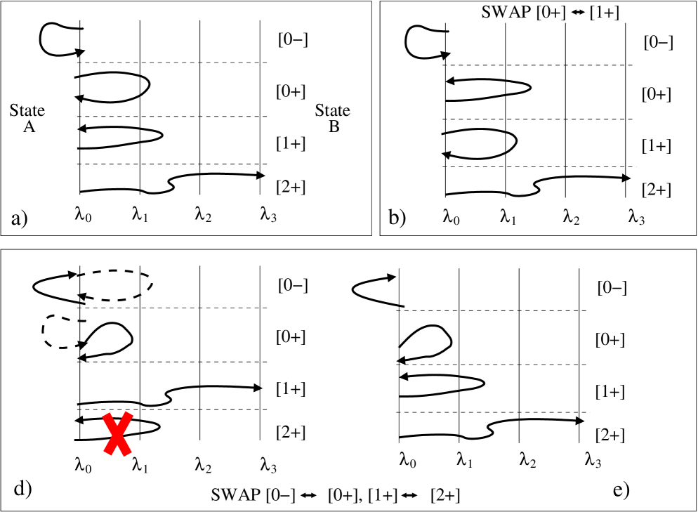
Figure 6: Parallel path swapping move in RETIS. The picture illustrates a RETIS simulation using four interfaces. a) shows the initial ”superstate” that contains one trajectory per ensemble $[0^{-}],[0^{+}],[1^{+}],$ and $[2^{+}]$. b) shows the superstate after the $[0^{+}]\leftrightarrow[1^{+}]$ swap. The original $[0^{+}]$ trajectory crossed $\lambda_{1}$ and is therefore a valid path in the $[1^{+}]$ ensemble. The swapping move is, therefore, accepted. c) shows the trial superstate that is obtained after the simultaneous swaps $[0^{-}]\leftrightarrow[0^{+}]$ and $[1^{+}]\leftrightarrow[2^{+}]$. The first swap requires the integration of motion forward or backward in time starting from the last of first timeslice of the swapped trajectories. This swap will always generate acceptable trajectories for the $[0^{-}],[0^{+}]$ ensembles. The other swap $[1^{+}]\leftrightarrow[2^{+}]$ is rejected because the old $[1^{+}]$ path does not cross $\lambda_{2}$. e) gives the final situation after the whole move.

The RETIS algorithm is then as follows. At each step it is decided by an equal probability whether a series of shooting or swapping moves will be performed. In the first case, all simulations will be updated sequentially by one shooting move. In the second case, again an equal probability will decide whether the swaps $[0^{-}]\leftrightarrow[0^{+}],[1^{+}]\leftrightarrow[2^{+}],\ldots$ or the swaps $[1^{+}]\leftrightarrow[2^{+}],[3^{+}]\leftrightarrow[4^{+}],\ldots$ are performed. Each time that $[0^{-}]$ and $[(n-1)^{+}]$ do not participate in the swapping move they are left unchanged. Also when the swapping move does not yield valid paths for both ensembles, the move is rejected for these two simulations and the old paths are counted again. Note that the swapping moves do not require any force calculations except for the $[0^{-}]\leftrightarrow[0^{+}]$ swap.

Like FFS, the path ensembles in RETIS are not fully uncorrelated. However, their dependence fundamentally different. In FFS, the path ensemble $[i^{+}]$ is fully determined by its predecessors, the MD simulation and the path simulations $[j^{+}]$ with $j<i$. Conversely, the separate RETIS simulations generate a large part of their trajectories independently. The exchange between the ensembles is, therefore, an additional help instead of a strict dependence as it is for FFS. Moreover, the benefit of the exchange works in both directions and is mutual for all ensembles, i. e. the $[i^{+}]$ path ensemble can improve the sampling in both $[(i+1)^{+}]$ and $[(i-1)^{+}]$ via the swapping moves $[i^{+}]\leftrightarrow[(i-1)^{+}]$ and $[i^{+}]\leftrightarrow[(i+1)^{+}]$, and will improve itself due to the same moves.

8 Numerical Example

We will apply the different methods on a simple one-dimensional test system using Langevin dynamics with finite friction. The Langevin dynamics was chosen because its inhibits stochasticity which is required for FFS. Hitherto, most studies on FFS have applied Brownian dynamics. As the dynamics we are considering are not overdamped, the dimensionality of the system becomes effectively two-dimensional. We could consider the velocity as an orthogonal coordinate (like $\lambda^{\perp}$ in Eq. 41). This makes the choice of a proper RC not such a triviality as one would think at first sight. However, we will simply take the RC to be configurational dependent, which is the standard approach. The system that we will consider consist of a single one-dimensional particle inside a double well potential

$$V(r)=k_{4}r^{4}-k_{2}r^{2}$$ (43)

with $k_{4}=1$ and $k_{2}=2$. The corresponding potential has a maximum at $r=0$ and two minima at $r=\pm 1$. We use reduced units where the mass and the Boltzmann constant are set to unity, $k_{B}=m=1$. The system is coupled to a Langevin thermostat with friction coefficient $\gamma=0.3$ and temperature $T=0.07$. The equations of motion are integrated using MD timestep of ${\mathrm{d}}t=0.002$. The RF method was applied using the EPF formalism for the transmission coefficient calculation. For this purpose 100,000 trajectories were released from the TST dividing surface $r=0$. The free energy term $\int_{-\infty}^{0}{\mathrm{d}}\lambda\,e^{-\beta F(\lambda)}$ was obtained by a simple numerical integration. The RF method is by far the most efficient method for this system because there is basically no error in the free energy calculation and the transmission coefficient is close to unity. The RF results will therefore be the reference for the other methods. The escape flux $f_{A}$ for TIS, FFS and PPTIS was determined using a MD simulation of 10,000,000 timesteps. The same MD result was used for these three methods. We performed an additional MD simulation using less timesteps, 4,000,000, for a second FFS calculation in order to see how this effects the final FFS result. I defined eight interfaces $\lambda_{0}=-0.9,\lambda_{1}=-0.8,\lambda_{2}=-0.7,\lambda_{3}=-0.6,\lambda_{4}=-0.5,\lambda_{5}=-0.4,\lambda_{6}=-0.3$, and $\lambda_{7}=1.0$. For each path ensemble 20,000 trajectories were generated. For TIS and PPTIS, 50% of the MC moves were shooting moves. I applied the aimless shooting [71] approach in which the velocities at the shooting point are completely regenerated from Maxwellian distribution. However, unlike Ref. [71], shooting points were picked with an equal probability for all timeslices along the path without considering the previous shooting point [9]. The other 50% were time-reversal moves. Time-reversal moves simply change the order of the timeslices of the old path while reversing the velocities. Time-reversal can sometimes increase the ergodic sampling and is basically cost-free as it doesnot require any force calculations. However, as aimless shooting is also able to reverse velocities in a single step, the time-reversal move could actually have been omitted for this case. In the RETIS algorithm there was at each step a 25% probability to perform a shooting move, another 25% probability to do a time-reversal move, and a 50% probability to do a replica exchange move. The FFS simulations consist of a single move which is the forward integration of the equations of motion. The Langevin thermostat served for the necessarily stochasticity. The results are shown in table 1. The RF method gives the most accurate results as expected. The value for $\kappa$ can be compared to Kramer’s expression $\kappa\approx(1/\omega_{b})(-\gamma/2+\sqrt{\gamma^{2}/4+\omega_{b}^{2}})=0.9$ with $\omega_{b}=\sqrt{k_{2}/m}=\sqrt{2}$.

Table 1: Results of the rate evaluations using RF, TIS, PPTIS, RETIS, and FFS. Final errors were obtained by block averaging and error-propagation rules. The errors of RETIS and FFS are given a star as these errors should not be considered exact due to the neglect of covariant terms which arise due the correlations between path ensembles and initial MD simulation. The FFS was repeated using a shorter (4,000,000 instead of 10,000,000 timesteps) initial MD run.

reactive flux method	$\frac{1}{\sqrt{2\pi\beta m}}$	$\frac{e^{-\beta F(0)}}{\int_{-\infty}^{0}{\mathrm{d}}\lambda\,e^{-\beta F(\lambda)}}$	$\kappa$	$k=\kappa\times\frac{1}{\sqrt{2\pi\beta m}}\times\frac{e^{-\beta F(0)}}{\int_{-\infty}^{0}{\mathrm{d}}\lambda\,e^{-\beta F(\lambda)}}$
EPF algorithm	0.106	$2.63\cdot 10^{-6}$	$0.874\pm 4\%$	$2.42\cdot 10^{-7}\pm$ 4 %
path sampling		$f_{A}$	${\mathcal{P}}_{A}(\lambda_{n}|\lambda_{0})$	k= $f_{A}\times{\mathcal{P}}_{A}(\lambda_{n}|\lambda_{0})$
TIS		$0.263\pm 1\%$	$1.52\cdot 10^{-6}\pm 20\%$	$4.02\cdot 10^{-7}\pm 20\%$
PPTIS		$0.263\pm 1\%$	$1.04\cdot 10^{-6}\pm 19\%$	$2.73\cdot 10^{-7}\pm 19\%$
RETIS		$0.265\pm 1\%^{*}$	$1.05\cdot 10^{-6}\pm 25\%^{*}$	$2.79\cdot 10^{-7}\pm 25\%^{*}$
FFS (long MD run)		$0.263\pm 1\%$	$4.69\cdot 10^{-8}\pm 6\%^{*}$	$1.23\cdot 10^{-8}\pm 6\%^{*}$
FFS (short MD run)		$0.259\pm 2\%$	$8.45\cdot 10^{-9}\pm 9\%^{*}$	$2.18\cdot 10^{-9}\pm 9\%^{*}$

If we compare the TIS, PPTIS, and RETIS simulations we see that they are all close (within a factor 2) to the RF result. The TIS result is somewhat too high which is probably due to a single path ensemble calculation that wasn’t fully converged after 20,000 steps. The RETIS results are clearly better despite the apparent errors that are somewhat smaller for TIS. The RETIS result is much closer to the RF reference. Moreover, it uses only halve the number of shooting moves compared to TIS, which is the most expensive move for realistic systems as it requires a large number of force evaluations. Also, the construction of the overall crossing probabilities in Fig. 7 shows a much better matching between the different ensembles in the RETIS method.

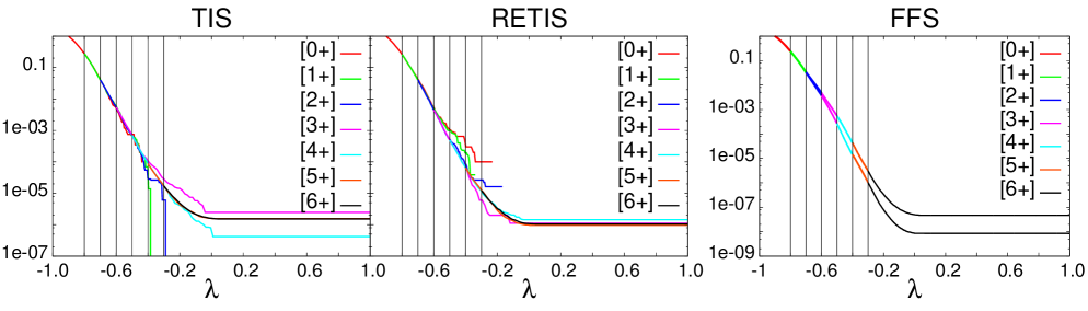
Figure 7: Overall crossing probabilities using TIS, RETIS, and FFS

The PPTIS result is also very close to the reference value. The PPTIS approximation, Eq. 32, becomes not only exact for very diffusive systems, but is also exact for steeply increasing barriers as all trajectories from $\lambda_{i}$ to $\lambda_{i+1}$ come directly from $\lambda_{0}$ in the past. FFS on the other hand, that is in principal exact unlike PPTIS, gives an unacceptable value that is about a factor 20 too low. Still, if we calculate the error using standard error propagation rules without taking care of the correlations between the ensembles [62], we get errors that seem very low. I also repeated the FFS simulation only changing the length of the initial MD simulation. A decrease of 60% for the initial MD simulation resulted in a final result that is again 5 times smaller. For TIS, PPTIS, and RETIS the impact of this MD reduction would not even be noticed as it only effects the error in the flux term that is negligible compared to the error in the crossing probability. Fig. 7 shows that the two different FFS crossing probabilities are similar at the start, but then start to deviate exponentially. The reason for this behavior is that the true set of reactive trajectories have an average kinetic energy distribution at the start that is considerably shifted compared to the equilibrium distribution. Therefore, a too short MD simulation might not generate sufficient crossing points having a high velocity. As result, the FFS trajectories mainly climb up the barrier helped by the stochastic force instead of a high initial velocity. In Fig. 8 we compare five randomly selected crossing trajectories for TIS and for FFS. The FFS trajectories are clearly unrealistic as they are not symmetric in the $(r,v)$ plane, which should be the case for a symmetric barrier. The velocities at the start are much lower than at the other side of the barrier. Moreover, two of the five trajectories, that were randomly picked from the 166 successful ones, start exactly from the same MD crossing point (from a total of 5260 crossing points). TIS, that is able to relax the history of the path, does not show this artefact.

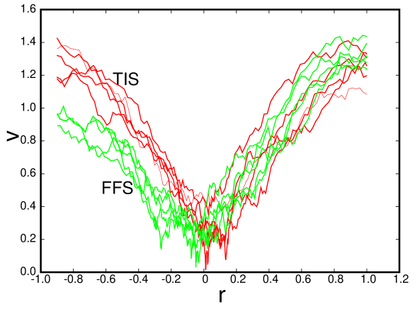
Figure 8: TIS and FFS trajectories in the $(r,v)$ plane

These results have important consequences. It shows that attempts to use FFS for deterministic MD [59, 60] by applying some small level of stochastic noise can only work when inertia effects are not important. In other words, when the deterministic dynamics behaves effectively Brownian. This sampling problem is not unique to FFS, but to any splitting-type method such as weighted ensemble Brownian dynamics [72, 73], Russian Roulette [57, 58], vector walking [74], and S-PRES [75], in which the equations of motion are only followed forward in time. There is not an easy solution for this problem. Still, this is very much desired for non-equilibrium systems for which there are no good alternatives. Possibly, the original nonequilibrium TPS approach of Crooks and Chandler [76] could do better in this situation as it continues rebuilding trajectories from the beginning. Still, the set of starting points follows from a straightforward MD trajectory. Therefore, also this approach is likely to miss these rare initial points that have high potential to become reactive. Timereversal moves might alleviate the problem [10], but can only be applied for time-reversible dynamics and velocity-symmetric steady state distributions. The other possibility is to adapt the RC, $\lambda(x)$, to the phasepoint committor, for instance via an on-the-fly optimization scheme [66]. Such an approach would need to be carried out in full phasespace, which is presently not the standard.

However, redefining the intermediate interfaces to lie on the isocommittor surfaces alone will not be sufficient. If we keep the $r$-dependent definition for stable state $A$, the committor probability can jump from zero to one is a single timestep (at the point when it leaves state $A$ with a high velocity). Hence, also the state definition $A$ should be redefined in phasespace. For this particular system it seems intuitive to use constant energy curves $\lambda(x)=1/2mv^{2}+V(r)$ as RC. FFS will probably work in that case., However, it is yet unclear if it is practically feasible to design appropriate RCs using full phasespace in more complex systems. Present algorithms [14] have always assumed that is sufficient to use configuration dependent committor functions.

On the other hand, the TIS methods seems to work properly using configuration dependent RCs. Only to ensure the stability of state $A$ it is sometimes convenient to let $\lambda_{0}$ be velocity dependent [8] (For this system, the friction coefficient is sufficiently high to neglect kineticly correlated recrossing). On the contrary, it seems that TIS and its variations do not necessarily improve when the RC equals the true isocommittor, a hypothesis that was postulated in Ref. [54]. If interfaces are places at constant energy curves, the trajectories will become much longer than in the present case.

9 Conclusions

I have reviewed some dynamical rare event simulation techniques. The RF method is likely the most efficient approach when studying low dimensional systems for which an appropriate RC can easily be found. The most efficient implementation of the RF approach to calculate the dynamical factor is probably the EPF algorithm that is considerably more efficient than the more common transmission coefficient calculation schemes. However, even with this more efficient EPF approach, the RF efficiency will decrease exponentially with barrier height and inverse temperature, if a proper RC can not be found [39]. The TPS reactive trajectory sampling does not require a RC. However, a definition of a RC is still needed in the TPS rate calculation algorithm, which has been improved by the TIS and RETIS methodologies. The TPS/TIS/RETIS efficiency only scales quadratically with barrier height and inverse temperature when using an ”improper” RC [39]. The RC insensitivity of these methods gives them a strong advantage compared to RF methods in complex systems. Of these methods, RETIS is significantly faster than the other two. However, its implementation is somewhat more difficult than TIS. PPTIS (and the similar milestoning) is not an exact method as it assumes memory loss beyond a traveling distance between two interfaces. Using this approximation, PPTIS is able to reduce the required path length considerably, which can be important for diffusive barrier crossings. FFS does not require information on the phasepoint density and is, therefore, ideally suited to study nonequilibrium events. The advantageous implementation and its apparent efficiency have made FFS a very popular method for equilibrium systems as well. However, the numerical study, presented here, shows that FFS has certain pitfalls that have not yet been reported. It shows that the RC sensitivity of FFS is even more troublesome than it is for RF methods. Present simulation studies have almost always assumed that RC are functions of configuration space alone. My example shows that an appropriate RC for FFS needs to be defined phasespace while configurational space would be sufficient for the RF method and the equilibrium path sampling algorithms TPS/(RE)TIS. Still, there are presently no alternative methods that can treat nonequilibrium processes and do not have the same problem. The fact that FFS and other forward MC methods get so easily trapped towards unfavorable reaction paths, by missing an important orthogonal coordinate or velocity in an early stage, requires the uppermost caution when applying these methods and interpreting their results. In addition, this article poses challenges for developing improved nonequilibrium path sampling methods that are either less sensitive to a chosen RC or are able to find an appropriate phasespace dependent RC on the fly.

Acknowledgments: TSvE acknowledges the Flemish Government for long-term structural support via the center of excellence (CECAT) and Methusalem funding (CASAS) and the support of the Interuniversity Attraction Pole (IAP-PAI).

10 List of abbreviations

EPF	Effective Positive Flux
FFS	Forward Flux Sampling
MC	Monte Carlo
MD	Molecular Dynamics
PPTIS	Partial Path Transition Interface Sampling
RC	Reaction Coordinate
RE	Replica Exchange
RETIS	Replica Exchange Transition Interface Sampling
RF	Reactive Flux method
TI	Thermodynamic Integration
TIS	Transition Interface Sampling
TPS	Transition Path Sampling
TS	Transition State
TST	Transition State Theory
US	Umbrella sampling

References

- [1] D. Chandler. Introduction to Modern Statistical Mechanics. Oxford University, New York, 1987.
- [2] D. Frenkel and B. Smit. Understanding molecular simulation, 2nd ed. Academic Press, San Diego, CA, 2002.
- [3] C. Dellago, P. G. Bolhuis, F. S. Csajka, and D. Chandler. Transition path sampling and the calculation of rate constants. J. Chem. Phys., 108:1964, 1998.
- [4] C. Dellago, P. G. Bolhuis, and D. Chandler. Efficient transition path sampling: Application to lennard-jones cluster rearrangements. J. Chem. Phys., 108:9236, 1998.
- [5] C. Dellago, P. G. Bolhuis, and D. Chandler. On the calculation of reaction rate constants in the transition path ensemble. J. Chem. Phys., 110:6617–6625, 1999.
- [6] P. G. Bolhuis, D. Chandler, C. Dellago, and P.L. Geissler. Transition path sampling: Throwing ropes over rough mountain passes, in the dark. Annu. Rev. Phys. Chem., 53:291–318, 2002.
- [7] C. Dellago, P. G. Bolhuis, and P. L. Geissler. Transition path sampling. Adv. Chem. Phys., 123:1–78, 2002.
- [8] T. S. van Erp, D. Moroni, and P. G. Bolhuis. A novel path sampling method for the sampling of rate constants. J. Chem. Phys., 118:7762–7774, 2003.
- [9] T. S. van Erp. Reaction rate calculation by parallel path swapping. Phys. Rev. Lett., 98(26):268301, 2007.
- [10] P. G. Bolhuis. Rare events via multiple reaction channels sampled by path repl ica exchange. J. Chem. Phys., 129:114108, 2008.
- [11] D. Moroni, P. G. Bolhuis, and T. S. van Erp. Rate constants for diffusive processes by partial path sampling. J. Chem. Phys., 120:4055–4065, 2004.
- [12] A. K. Faradjian and R. Elber. Computing time scales from reaction coordinates by milestoning. J. Chem. Phys., 120:10880, 2004.
- [13] R. J. Allen, P. B. Warren, and P. R. ten Wolde. Sampling rare switch ing events in biochemical networks. Phys. Rev. Lett., 94:018104, 2005.
- [14] C. Dellago and P. G. Bolhuis. Transition path sampling and other advanced simulation techniques for rare events. In Advanced Computer Simulation Approaches for Soft Matter Sciences III, volume 221 of Advances in Polymer Science, pages 167–233. 2009.
- [15] F. A. Escobedo, E. E. Borrero, and J. C. Araque. Transition path sampling and forward flux sampling. applications to biological systems. J. Phys.-Condes. Matter, 21:333101, 2009.
- [16] R. J. Allen, C. Valeriani, and P. R. ten Wolde. Forward flux sampling for rare event simulations. J. Phys.-Condes. Matter, 21:463102, 2009.
- [17] P. G. Bolhuis and C. Dellago. Trajectory-based rare event simulations. In Reviews in Computational Chemistry. San Diego, CA, 2010.
- [18] P. Hanggi, P. Talkner, and M. Borkovec. Reaction-rate theory - 50 years after Kramers. Rev. Mod. Phys., 62:251–341, 1990.
- [19] B. J. Alder and T. E. Wainwright. Phase transition for a hard sphere system. J. Chem. Phys., 27:1208, 1957.
- [20] H. Eyring. The activated complex in chemical reactions. J. Chem. Phys., 3:107, 1935.
- [21] E. Wigner. The transition state method. Trans. Faraday Soc., 34:29, 1938.
- [22] J. C. Keck. Statistical investigation of dissociation cross-section for diatoms. Discuss. Faraday Soc., 33:173, 1962.
- [23] C. H. Bennett. Molecular dynamics and transition state theory: the simulation of infrequent events. In R.E. Christofferson, editor, Algorithms for Chemical Computations, ACS Symposium Series No. 46, Washington, D.C., 1977. American Chemical Society.
- [24] D. Chandler. Statistical-mechanics of isomerization dynamics in liquids and transition-state approximation. J. Chem. Phys., 68:2959–2970, 1978.
- [25] T. Yamamoto. Quantum statistical mechanical theory of the rate of exchange chemical reactions in the gas phase. J. Chem. Phys., 33:281, 1960.
- [26] J. Horiuti. On the statistical mechanical treatment of the absolute rate of the chemical reaction. Bull. Chem. Soc. Jpn, 13:210, 1938.
- [27] G. M. Torrie and J. P. Valleau. Monte-Carlo free-energy estimates using non-Boltzmann sampling - application to subcritical Lennard-Jones fluid. Chem. Phys. Lett., 28:578, 1974.
- [28] E. A. Carter, G. Ciccotti, J. T. Hynes, and R. Kapral. Constrained reaction coordinate dynamics for the simulation of rare events. Chem. Phys. Lett., 156:472, 1989.
- [29] D. Moroni. Efficient sampling of rare events. PhD thesis, Universiteit van Amsterdam, 2005.
- [30] S. Kumar, D. Bouzida, R. H. Swendsen, P. A. Kollman, and J. M. Rosenberg. the Weighted Histogram Analysis Method for Free-Energy Calculations on Biomolecules .1. The Method. J. Comput. Chem., 13(8):1011–1021, 1992.
- [31] W. K. den Otter and W. J. Briels. The calculation of free-energy differences by constrained molecular-dynamics simulations. J. Chem. Phys., 109(11):4139–4146, 1998.
- [32] H. Grubmüller. Predicting slow structural transitions in macromolecular systems - conformational flooding. Phys. Rev. E, 52:2893–2906, 1995.
- [33] E. Darve and A. Pohorille. Calculating free energies using average force. J. Chem. Phys., 115(20):9169–9183, 2001.
- [34] F. G. Wang and D. P. Landau. Efficient, multiple-range random walk algorithm to calculate the density of states. Phys. Rev. Lett., 86:2050–2053, 2001.
- [35] A. Laio and M. Parrinello. Escaping free-energy minima. Proc. Natl. Acad. Sci. USA, 99:12562, 2002.
- [36] J. B. Anderson. Predicting rare events in molecular dynamics. Adv. Chem. Phys., 91:381–431, 1995.
- [37] T. S. van Erp. Solvent effects on chemistry with alcohols. PhD thesis, Universiteit van Amsterdam, 2003.
- [38] E. Vanden-Eijnden and F. A. Tal. Transition state theory: Variational formulation, dynamical corrections, and error estimates. J. Chem. Phys., 123:184103, 2005.
- [39] T. S. van Erp. Efficiency analysis of reaction rate calculation methods using analytical models I: The two-dimensional sharp barrier. J. Chem. Phys., 125(17):174106, 2006.
- [40] T. S. van Erp and P. G. Bolhuis. Elaborating transition interface sampling methods. J. Comput. Phys., 205:157–181, 2005.
- [41] G. W. N. White, S. Goldman, and C. G. Gray. Test of rate theory transmission coefficients algorithms. an application to ion channels. Mol. Phys., 98:1871–1885, 2000.
- [42] M. J. Ruiz-Montero, D. Frenkel, and J. J. Brey. Efficient schemes to compute diffusive barrier crossing rates. Mol. Phys., 90:925–941, 1997.
- [43] T. S. van Erp and E. J. Meijer. Proton assisted ethylene hydration in aqueous solution. Angew. Chemie, 43:1659–1662, 2004.
- [44] K. V. Klenin and W. Wenzel. A method for the calculation of rate constants from stochastic transition paths. J. Chem. Phys., 132(10):104104, MAR 14 2010.
- [45] J. Rogal and P. G. Bolhuis. Multiple state transition path sampling. J. Chem. Phys., 129(22):224107, 2008.
- [46] D. Ryter. On the eigenfunctions of the Fokker-Planck operator and of its adjoint. Physica A, 142(1-3):103–121, 1987.
- [47] B. Peters, G. T. Beckham, and B. L. Trout. Extensions to the likelihood maximization approach for finding reaction coordinates. J. Chem. Phys., 127:034109, 2007.
- [48] E. Vanden-Eijnden. Transition path theory. In M Ferrario, G Ciccotti, and K Binder, editors, Computer Simulations in Condensed Matter Systems: From Materials to Chemical Biology, volume 703 of Lecture Notes in Physics, pages 453–493, New York, US, 2006. Springer.
- [49] W. E and E. Vanden-Eijnden. Transition-Path Theory and Path-Finding Algorithms for the Study of Rare Events. volume 61 of Annual Review of Physical Chemistry, pages 391–420. 2010.
- [50] A. N. Drozdov and S. C. Tucker. An improved reactive flux method for evaluation of rate constants in dissipative systems. J. Chem. Phys., 115(21):9675–9684, 2001.
- [51] T. S. Van Erp, T. P. Caremans, C. E. A. Kirschhock, and J. A. Martens. Prospects of transition interface sampling simulations for the theoretical study of zeolite synthesis. Phys. Chem. Chem. Phys., 9(9):1044–1051, 2007.
- [52] D. T. Gillespie. Monte-Carlo simulation of random-walks with residence time-dependent transition-probability rates. J. Comput. Phys., 28:395, 1978.
- [53] A. Aerts, M. Haouas, T. P. Caremans, L. R. A. Follens, T. S. van Erp, F. Taulelle, J. Vermant, J. A. Martens, and C. E. A. Kirschhock. Investigation of the Mechanism of Colloidal Silicalite-1 Crystallization by Using DLS, SAXS, and Si-29 NMR Spectroscopy. Chem.-Eur. J., 16:2764–2774, 2010.
- [54] E. Vanden-Eijnden, M. Venturoli, G. Ciccotti, and R. Elber. On the assumptions underlying milestoning. J. Chem. Phys., 129(17):174102, 2008.
- [55] D. Moroni, T. S. van Erp, and P. G. Bolhuis. Simultaneous computation of free energies and kinetics of rare events. Phys. Rev. E, 71:056709, 2005.
- [56] P. Majek and R. Elber. Milestoning without a reaction coordinate. J. Chem. Theory Comput., 6:1805–1817, 2010.
- [57] T. E. Booth and J. S. Hendricks. Importance estimation in forward Monte-Carlo calculations. Nucl. Techno.-Fus., 5(1):90–100, 1984.
- [58] P. G. Melnik-Melnikov and E. S. Dekhtyaruk. Rare events probabilities estimation by “Russian Roulette and Splitting” simulation technique. Probab. Eng. Eng. Mech., 15(2):125–129, APR 2000.
- [59] Z.-J. Wang, C. Valeriani, and D. Frenkel. Homogeneous Bubble Nucleation Driven by Local Hot Spots: A Molecular Dynamics Study. J. Phys. Chem. B, 113(12):3776–3784, 2009.
- [60] C. Velez-Vega, E. E. Borrero, and F. A. Escobedob. Kinetics and reaction coordinate for the isomerization of alanine dipeptide by a forward flux sampling protocol. J. Chem. Phys., 130(22):225101, 2009.
- [61] P. G. Bolhuis. Transition path sampling on diffusive barriers. J. Phys. Cond. Matter, 15:S113–S120, 2003.
- [62] R. J. Allen, D. Frenkel, and P. R. ten Wolde. Forward flux sampling-type schemes for simulating rare events: Efficiency analysis. J. Chem. Phys., 124:194111, 2006.
- [63] J. Juraszek and P. G. Bolhuis. Rate Constant and Reaction Coordinate of Trp-Cage Folding in Explicit Water. Biophys. J., 95(9):4246–4257, 2008.
- [64] R. P. Sear. Nucleation in the presence of slow microscopic dynamics. J. Chem. Phys., 128(21):214513, 2008.
- [65] E. Sanz, C. Valeriani, D. Frenkel, and M. Dijkstra. Evidence for out-of-equilibrium crystal nucleation in suspensions of oppositely charged colloids. Phys. Rev. Lett., 99(5):055501, AUG 3 2007.
- [66] E. E. Borrero, L. M. Contreras Martinez, M. P. DeLisa, and F. A. Escobedo. Kinetics and Reaction Coordinates of the Reassembly of Protein Fragments Via Forward Flux Sampling. Biophys. J., 98(9):1911–1920, 2010.
- [67] T. S. van Erp. Efficient path sampling on multiple reaction channels. Comput. Phys. Commun., 179:34–40, 2008.
- [68] R. H. Swendsen and J. S. Wang. Replica Monte-Carlo simulation of spin-glasses. Phys. Rev. Lett., 57:2607–2609, 1986.
- [69] E. Marinari and G. Parisi. Simulated tempering - a new monte-carlo scheme. Europhysics Lett., 19(6):451–458, 1992.
- [70] T. J. H. Vlugt and B. Smit. On the efficient sampling of pathways in the transition path ensemble. Phys. Chem. Comm., 2:1–7, 2001.
- [71] B. Peters and B. L. Trout. Obtaining reaction coordinates by likelihood maximization. J. Chem. Phys., 125(5), 2006.
- [72] G. A. Huber and S. Kim. Weighted-ensemble Brownian dynamics simulations for protein association reactions. Biophys. J., 70(1):97–110, 1996.
- [73] B. W. Zhang, D. Jasnow, and D. M. Zuckerman. Efficient and verified simulation of a path ensemble for conformational change in a united-residue model of calmodulin. Proc. Natl. Acad. Sci. USA, 104(46):18043–18048, 2007.
- [74] S. Tănase-Nicola and J. Kurchan. Topological methods for searching barriers and reaction paths. Phys. Rev. Lett., 91:188302, 2003.
- [75] J. T. Berryman and T. Schilling. Sampling rare events in nonequilibrium and nonstationary systems. J. Chem. Phys., 133:244101, 2010.
- [76] G. E. Crooks and D. Chandler. Efficient transition path sampling for nonequilibrium stochastic dynamics. Phys. Rev. E, 64:026109, 2001.