Subsampling Methods for genomic inference

Abstract

Large-scale statistical analysis of data sets associated with genome sequences plays an important role in modern biology. A key component of such statistical analyses is the computation of $p$-values and confidence bounds for statistics defined on the genome. Currently such computation is commonly achieved through ad hoc simulation measures. The method of randomization, which is at the heart of these simulation procedures, can significantly affect the resulting statistical conclusions. Most simulation schemes introduce a variety of hidden assumptions regarding the nature of the randomness in the data, resulting in a failure to capture biologically meaningful relationships. To address the need for a method of assessing the significance of observations within large scale genomic studies, where there often exists a complex dependency structure between observations, we propose a unified solution built upon a data subsampling approach. We propose a piecewise stationary model for genome sequences and show that the subsampling approach gives correct answers under this model. We illustrate the method on three simulation studies and two real data examples.

T1Supported by NIH U01 HG004695 (ENCODE DAC) and NIH 5R01GM075312. , , , and

[*]t1The authors are ordered alphabetically.

1 Introduction

1.1 Background

This paper grew out of a number of examples arising in data coming from the Encyclopedia of DNA Elements (ENCODE) Pilot Project [Birney et al. (2007)], which is composed of multiple, diverse experiments performed on a targeted 1% of the human genome. Computational analyses of this data are aimed at revealing new insights about how the information coded in the DNA blueprint is turned into functioning systems in the living cell. Variations of some of the methods described here have been applied at various places in that paper, as well as in Margulies et al. (2007), for assessing significance and computing confidence bounds for statistics that operate along a genomic sequence. The background of these methods is described in cookbook form in the supplements to those papers, and it is the goal of this paper to present them rigorously and to develop some necessary refinements.

Essentially, we will argue that, in making inference about statistics computed from “large” stretches of the genome, in the absence of real knowledge about the evolutionary path which led to the genome in question, the best we can do is to model the genome by a piecewise stationary ergodic random process. The variables of this process can be base pair composition or some other local features, such as various annotated functional elements.

In the purely stationary case some of the types of questions that we will address, such as tests for independence of point processes, confidence bounds for expectations of local functions and goodness of fit of models, have been considered extensively. However, inference for piecewise stationary models appears not to have been investigated. With the advent of enormous amounts of genomic data, all sorts of inferential questions have arisen. The proposed model may be the only truly nonparametric approach to the genome, although, just as in ordinary nonparametric statistics, there are many possible ways of carrying out inference.

Our methods are based on a development of the resampling schemes of Politis and Romano (1994), Politis, Romano and Wolf (1999) and the block bootstrap methods of Künsch (1989). As we shall see, in many situations, Gaussian approximations can replace these schemes. But in these situations, as with the ordinary bootstrap, we believe that a subsampling approach is valuable for the following reasons:

• Letting the computer do the approximation is much easier.

• Some statistics, such as tests of the Kolmogorov–Smirnov type, are functions of stochastic processes to which a joint Gaussian approximation applies. Then, limiting distributions can only be computed by simulation.

• The bootstrap distributions of our statistics show us whether the approximate Gaussianity we have invoked for the “true” distribution of these statistics is in fact warranted. This visual confirmation is invaluable.

This paper is organized as follows. We begin with some concrete examples from the ENCODE data as well as other types of genomic data in Section 1.2, and proceed with a motivated description of our model in Section 2. Our methods are discussed both qualitatively and mathematically in Sections 3 and 4. Section 5 contains results from simulation studies and real data analysis. Proofs of theorems stated in Sections 3 and 4 can be found in the supplemental article [Bickel et al. (2010)].

The statistics and methods discussed in this paper have been implemented in several computing languages and are available for download at http://www.encodestatistics.org/. Each of these implementations runs in $n\log(n)$ time, where $n$ is the number of instances of the more frequent feature. On a desktop PC (Intel Core Duo 3 GHz and 2 Gb RAM) the Python version takes over 1000 samples per second for features on the order of $10^{4}$ instances.

1.2 Motivating examples

We start with several fundamental questions that arise in genomic studies.

• Association of functional elements in genomes. In genomic analyses, a natural quantity of interest is the association among different functional sites/features annotated along the DNA sequence. Its biological motivation comes from the common belief that significant physical overlapping or proximity of functional sites in the genome suggests biological constraints or relationships. In the ENCODE project, to understand the possible functional roles of the evolutionarily constrained sequences that are conserved across multiple species, overlap between the constrained sequences and several experimental annotations, such as 5’UTR, RxFrags, pseudogenes, and coding sequences (CDSs), have been evaluated using the method discussed in this paper. It was found that the overlap of most experimental annotations with the constrained sequences are significantly different from random [Birney et al. (2007)]. An illustrative example from The ENCODE Project [Birney et al. (2007)] is detailed in Section 5.1.

• Cooperativity between transcription factor binding sites. In some situations, there is interest to study the associations between neighboring functional sites that do not necessarily overlap. For instance, it is known that transcription factors often work cooperatively and their binding sites (TFBS) tend to occur in clusters [Zhang et al. (2006)]. Consequently, methods for identifying interacting transcription factors usually involve evaluating the significance of co-occurrences of their binding sites in a local genomic region [Zhou and Wong (2004); Das, Banerjee and Zhang (2004); Yu, Yoo and Greenwald (2004); Huang et al. (2004); Kato et al. (2004); Gupta and Liu (2005)]. This problem has the same formulation as the above ENCODE examples given a functional site defined as follows: for a TFBS of length $l$ at position $i$, we define the region $(i-m,i+l+m)$ as a functional site. Then two overlapping functional sites are equivalent to two neighboring TFBSs with interdistance less than $2m$, and the methods discussed in this paper for evaluating the significance of overlapping functional features can be applied. We leave this and related applications which involve considering statistics of the K-S type to a later paper.

• Correlating DNA copy number with genomic content. Recent technology has made it possible to assay DNA copy number variation at a very fine scale along the genome [for review, see Carter (2007)]. Many studies, for example, Redon et al. (2006), have shown that such variation in DNA copy number is a common type of polymorphism in the human genome. To what extent do these regions of copy number changes overlap with known genomic features, such as coding sequences? Redon et al. performed such an analysis and argued that copy number variant regions have a significant paucity for coding regions. The $p$-values supporting this claim were based on random permutations of the start locations of the variant segments. This assumes uniformity and stationarity of the copy number variants. However, CNVs do not occur at random and are often clustered in regions of the genome containing segmental duplications. The methods discussed in this paper for evaluating the significance of overlapping features, which assume neither uniformity nor stationarity, can again be applied to this problem. Actually, the results from our method suggest a different conclusion on this problem (see Section 5.5).

As we have seen in these examples, a common question asked in many applications is the following: Given the position vectors of two features in the genome, for example, “conservation between species” and “transcription start sites,” and a measure of relatedness between features, for example, base or region percentage overlap, how significant is the observed value of the measure? How does it compare with that which might be observed “at random?”

The essential challenge in the statistical formulation of this problem is the appropriate modeling of randomness of the genome, since we observe only one of the multitudes of possible genomes that evolution might have produced for our and other species.

How have such questions been answered previously? Existing methods employ varied ways to simulate the locations of features within genomes, but all center around the uniformity assumption of the features’ start positions: The features must occur homogeneously in the studied genome region, for example, Blakesley et al. (2004) and Redon et al. (2006). This assumption ignores the natural clumping of features as well as the nonstationarity of genome sequences. Clumping of features is quite common along the genome due to either the feature’s own characteristic, for example, transcription factor binding sites (TFBSs) tend to occur in clusters, or the genome’s evolutionary constraints, for example, conserved elements are often found in dense conservation neighborhoods. Ignoring these natural properties could result in misleading conclusions.

In this paper we suggest a piecewise stationary model for the genome (see Section 2) and, based on it, propose a method to infer the relationships between features which we view as “nonparametric” as possible (see Sections 4.2 and 4.4). The model is based on assumptions which we demonstrate in real data examples to be plausible.

2 The piecewise stationary model

2.1 Genomic motivation

We postulate the following for the observed genomes or genomic regions:

• They can be thought of as a concatenation of a number of regions, each of which is homogenous in a way we describe below.

• Features that are located very far from each other on the average have little to do with each other.

• The number of such homogeneous regions is small compared to the total length of the observed genome.

These assumptions, which form the underpinning of our block stationary model for genomic features, are motivated by earlier studies of DNA sequences, which show that there are global shifts in base composition, but that certain sequence characteristics are locally unchanging. One such characteristic is the GC content. Bernardi et al. (1985) coined the term “isochore” to denote large segments (of length greater than 300 Kb) that have fairly homogeneous base composition and, especially, constant GC composition. Even earlier, evidence of segmental DNA structure can be found in chromosomal banding in polytene chromosomes in drosophila, visible through the microscope, that result from underlying physical and chemical structure. These banding patterns are stable enough to be used for the identification of chromosomes and for genetic mapping, and are physical evidence for a block stationarity model for the GC content of the genome.

The experimental evidence for segmental genome structure and the increasing availability of DNA sequence data have inspired attempts to computationally segment DNA into statistically homogeneous regions. The paper by Braun and Müller (1998) offers a review of statistical methods developed for detecting and modeling the inhomogeneity in DNA sequences. There have been many attempts to segment DNA sequences by both base composition [Fu and Curnow (1990); Churchill (1989, 1992); Li et al. (2002)] and chemical characteristics [Li et al. (1998)]. Most of these computational studies concluded that a model that assumes block-wise stationarity gives a significantly better fit to the data than stationary models [see, for example, the conclusions of two very different studies by Fickett, Torney and Wolf (1992) and Li et al. (1998)].

A subtle issue in the definition of “homogeneity” is the scale at which the genome is being analyzed. Inhomogeneity at the kilobase resolution, for example, might be “smoothed out” in an analysis at the megabase level. The level of resolution is a modeling issue that must be considered carefully with the goal of the analysis in mind.

Implicit in our formulation is an “ergodic” hypothesis. We want probabilities to refer to the population of potential genomes. We assume that the statistics of the genome we have mimic those of the population of genomes. This is entirely analogous to the ergodic hypothesis that long term time averages agree with space averages for trajectories of dynamic systems.

2.2 Mathematical formulation

In mathematical terms, the block stationarity model assumes that we observe a sequence of random variables $\{X_{1},\dots,X_{n}\}$ positioned linearly along the genomic region of interest. $X_{k},k=1,\ldots,n,$ may be base composition, or some other measurable feature. We assume that there exist integers $\bolds{\tau}=\bolds{\tau}^{(n)}=(\tau_{0},\dots,\tau_{U})$, where $0=\tau_{0}<\tau_{1}<\cdots<\tau_{U}=n$, such that the collections of variables, $\{X_{\tau_{i}},\ldots,X_{\tau_{i+1}}\}$, are separately stationary for each $i=0,\dots,U-1$. We let $n_{i}=\tau_{i}-\tau_{i-1}$ be the length of the $i$th region, and let there be $U$ such regions in total. For convenience, we introduce the mapping

$$\pi\dvtx\{1,\dots,n\}\rightarrow\{(i,j)\dvtx 1\leq i\leq U,1\leq j\leq n_{i}\}$$

which relates the relabeled sequence, $\{X_{ij}\dvtx 1\leq i\leq U,1\leq j\leq n_{i}\}$, to the original sequence $\{X_{1},\ldots,X_{n}\}$. We write $\pi=(\pi_{1},\pi_{2})$ with $\pi(k)=(i,j)$ if and only if $k=\tau_{i}+j$. We will use the notation $X_{ij}$ and $X_{k}$ interchangeably throughout this paper.

For any $k_{1}$, $k_{2}$, let $\mathcal{F}_{k_{1}}^{k_{2}}$ be the $\sigma$-field generated by $X_{k_{1}},\dots,X_{k_{2}}$. Define $m(k)$ to be the standard Rosenblatt mixing number [Dedecker et al. (2007)],

$$m(k)=\sup\{|\mathbb{P}(AB)-\mathbb{P}(A)\mathbb{P}(B)|\dvtx A\in\mathcal{F}_{1}^{l},B\in\mathcal{F}_{l+k}^{n},1\leq l\leq n-k\}.$$

Then, assumptions 1–3 stated in Section 2.1 translate to the following:

1. [A1.]

2. The sequence $\{X_{1},\ldots,X_{n}\}$ is piecewise stationary. That is, $\{X_{ij}\dvtx 1\leq j\leq n_{i}\}$ is a stationary sequence for $i=1,\dots,U$.

3. There exists constants $c$ and $\beta>0$ such that $m(k)\leq ck^{-\beta}$ for all $k$.

4. $U/n\rightarrow 0$.

An immediate and important consequence of A1–A3 is that, for any fixed small $k$, if we define $W_{1}=(X_{1},\ldots,X_{k}),W_{2}=(X_{k+1},\ldots,X_{2k}),\ldots,W_{m}=(X_{n-k+1},\ldots,X_{n})$, where $m=n/k$, then $\{W_{1},\ldots,W_{m}\}$ also obey A1–A3. This is useful, for example, in the region overlap example considered in the next section.

The remarkable feature of these assumptions, which are more general to our knowledge than any made heretofore in this context, is that they still allow us to conduct most of the statistical inference of interest. Not surprisingly, these assumptions lead to more conservative estimates of significance than any of the previous methods.

3 Vector linear statistics and Gaussian approximation

We study the distribution of a class of vector linear statistics of interest under the above piecewise stationary model. As an illustration, we consider the ENCODE data examples, and suppose that we are interested in base pair overlap between features $A$ and $B$. We can represent base pair overlap by defining

$$I_{k}=1,\qquad\mbox{if position $k$ belongs to feature $A$ and $0$ otherwise},$$

$$J_{k}=1,\quad\hskip 10.0pt\mbox{if position $k$ belongs to feature $B$ and $0$ otherwise}.$$

We can then define $X_{k}=I_{k}J_{k}$ to be the indicator that position $k$ belongs to both features $A$ and $B$. Then, for the $n=30$ megabases of the ENCODE regions, the mean base pair overlap is equal to

$$\bar{X}=\sum_{k=1}^{n}X_{k}/n.$$

Another biologically interesting statistic is the (asymmetric) region overlap, defined as follows: suppose the consecutive feature stretches are $T_{1},\ldots,T_{\alpha}$ with lengths $\tau_{1},\ldots,\tau_{\alpha}$, and the corresponding nonfeature stretches $S_{1},\ldots,S_{\beta}$ with lengths $\rho_{1},\ldots,\rho_{\beta}$. We assume here that the initial and final stretches consist of one feature and one nonfeature stretch. The complementary situation, when both initial and final stretches are of the same type, is dealt with similarly. Without loss of generality, suppose the initial stretch is nonfeature. Then, $S_{1}=\{1,\ldots,\rho_{1}\}$, $T_{1}=\{\rho_{1}+1,\ldots,\rho_{1}+\tau_{1}\}$, $S_{2}=\{\rho_{1}+\tau_{1}+1,\ldots,\rho_{1}+\tau_{1}+\rho_{2}\}$, etc. Using $I_{k}$, $J_{k}$ as indicators of feature identity, we define the (unnormalized) region overlap of feature $A$ stretches with feature $B$ stretches as $\frac{1}{n}\sum_{t=1}^{\alpha}V_{t}$ where $V_{t}=1-\prod_{k\in T_{A,t}}(1-J_{k})$, where $T_{A,1},\ldots,T_{A,\alpha}$ denote the feature $A$ stretches. This statistic is not linear in terms of functions of single basepairs, but is linear in functions of blocks of feature $B$. These blocks are of random sizes, but are consistent with our hypothesis of piecewise stationarity that, except for end effects due to feature instances crossing segment boundaries, the ${V_{t}}$ are also stationary. If the lengths $\tau_{1},\ldots,\tau_{\alpha}$ are negligible compared to $n$ and $\alpha$ is of the order of $n$, we can expect the mixing hypothesis to remain valid.

In general, we focus our attention on statistics that can be expressed as a function of the mean of $\mathbf{g}(X_{i})$, where $\mathbf{g}$ is some well behaved $d$-dimensional vector function to be characterized in later sections. By the flexible definition of $\mathbf{g}$, this encompasses a wide class of situations.

First, we consider vector linear statistics of the form

$$\mathbf{T}_{n}(\mathbf{X})=n^{-1}\sum_{k=1}^{n}\mathbf{g}(X_{k}).$$

We introduce the following notation:

$$E[\mathbf{T}_{n}]\equiv\bolds{\mu}\equiv\sum_{i=1}^{U}f_{i}\bolds{\mu}_{i},$$

where

$$\bolds{\mu}_{i} \equiv E[\mathbf{g}(X_{i1})],$$

$$f_{i} \equiv n_{i}/n$$

and

$$\Sigma_{n}\equiv\operatorname{\mathbb{V}ar}(n^{{1/2}}\mathbf{T}_{n})=\sum^{U}_{i=1}f_{i}C_{i}(nf_{i}),$$ (1)

where

$$C_{i}(m)=C_{i0}+2\sum^{m}_{\ell=1}C_{i\ell}\biggl{(}1-\frac{(\ell-1)}{m}\biggr{)}$$

and

$$C_{i0}\equiv\operatorname{\mathbb{V}ar}\mathbf{g}(X_{1}),\qquad C_{i\ell}\equiv\operatorname{\mathbb{C}ov}\bigl{(}\mathbf{g}(X_{i1}),\mathbf{g}\bigl{(}X_{i(l+1)}\bigr{)}\bigr{)}.$$ (2)

In Theorem 3.1 below, we show asymptotic Gaussianity of $\mathbf{T}_{n}$ given a few more technical assumptions:

1. [A4.]

2. $\frac{1}{n}\sum_{i:n_{i}\leq l}n_{i}\rightarrow 0$ for all $l<\infty$.

3. $\forall i$, $|\mathbf{g}|_{\infty}\leq C<\infty$.

4. $0<\varepsilon_{0}\leq\|\Sigma_{n}\|\leq\varepsilon_{0}^{-1}$, for all $n$, where $\|\cdot\|$ is a matrix norm.

In particular, A4 implies that the contribution of “small regions” to the overall statistic must not be too large.

Theorem 3.1

Under conditions A1–A6,

$$n^{{1/2}}\Sigma_{n}^{-{1/2}}(\mathbf{T}_{n}-\bolds{\mu})\Rightarrow\mathcal{N}(\mathbf{0},\mathbf{I}),$$ (3)

where $\mathbf{I}$ is the $d\times d$ identity.

The proof of the theorem is in the supplemental article [Bickel et al. (2010)]. If we have estimates $\hat{\bolds{\tau}}$ of $\bolds{\tau}$ which are consistent in a suitably uniform sense, then estimates of $C_{i\ell}$, $C_{i}(m)$ using $\hat{\bolds{\tau}}$ in place of $\bolds{\tau}$ are also consistent. However, simply plugging these estimates into (1) does not yield consistent estimates of $\sigma^{2}$ if our approach were to compute confidence intervals by Gaussian approximation. This is well known for the stationary case. Some regularization is necessary. We do not pursue this direction but prefer to approach the inference problem from a resampling point of view—see next section.

In many cases, the statistics of interest are not linear. For example, in the analysis of the ENCODE data a more informative statistic is the %bp overlap defined as

$$B\equiv\frac{\bar{X}}{D},$$ (4)

where

$$D=\sum_{k=1}^{n}I_{k}$$

is the total base count of feature $A$.

More conceptually, the region overlap is

$$R\equiv\frac{1}{W_{I}}\sum_{k=1}^{K}V_{k},$$ (5)

where $W_{I}=\sum_{k=1}^{n}I_{k-1}(1-I_{k})$, the number of feature $A$ instances.

A standard delta method computation shows that the standard error of $B$ can be approximated as follows: Let $\mu(D)$ and $\mu(\bar{X})$ be respectively the expectation of $D$ and $\bar{X}$. Then,

$$\frac{\bar{X}}{D}-\frac{\mu(\bar{X})}{\mu(D)}\approx\frac{\bar{X}-\mu(\bar{X})}{\mu(D)}-\mu(\bar{X})\frac{(D-\mu(D))}{\mu^{2}(D)},$$

and, hence, we can approximate $\frac{\bar{X}}{D}$ by a Gaussian variable with mean $\frac{\mu(\bar{X})}{\mu(D)}$ and variance

$$\sigma^{2}(B)\approx\frac{\sigma^{2}(\bar{X})}{\mu^{2}(D)}+\frac{\mu^{2}(\bar{X})}{\mu^{4}(D)}\sigma^{2}(D)-2\frac{\mu(\bar{X})}{\mu^{3}(D)}\operatorname{Cov}(\bar{X},D),$$ (6)

where $\sigma^{2}(B)$, $\sigma^{2}(\bar{X})$, $\sigma^{2}(D)$ are the corresponding variances and $\operatorname{Cov}(\bar{X},D)$ denotes the covariance. In doing inference, we can use the approximate Gaussianity of $B$ with $\sigma^{2}(B)$ estimated using the above formula with regularized sample moments replacing the true moments.

We also note that goodness of fit or equality of population test statistics, such as Kolmogorov–Smirnov and many others, can be viewed as functions of empirical distributions, which themselves are infinite-dimensional linear statistics, and we expect, but have not proved, that the methods discussed in this paper and the underlying theories apply to those cases as well, under suitable assumptions.

4 Subsampling based methods

Here we propose a subsampling based approach, in particular, a combined segmentation-block subsampling method to conduct statistical inference under the piecewise stationary model, which we call “segmented block subsampling.” In our method, the segmentation parameters governing scale are chosen first and then the size of the subsample is chosen based on stability criteria. The segmentation procedure, as we discussed, is motivated by the heterogeneity of large-scale genomic sequences. The block subsampling approach takes into account the local genomic structure, such as natural clumping of features, when conducting statistical inference. We explicitly demonstrate the advantages of using segmentation and block subsampling by simulation studies in Section 5.

4.1 Stationary block subsampling

Below we first review the results related to the stationary block bootstrap method in a homogeneous region ($U=1$), and then show how the method breaks down when it is applied to a piecewise stationary sequence ($U>1$).

4.1.1 Review of results for the case of $U=1$

For completeness, we recall the following basic algorithm of Politis and Romano (1994) to obtain an estimate of the distribution of the statistic $\mathbf{T}_{n}(X_{1},\ldots,X_{n})$ under the assumption that the sequence $X_{1},\ldots,X_{n}$ is stationary (i.e., $U=1$).

Algorithm 4.1.

(a) Given $L\ll n$ choose a number $N$ uniformly at random from $\{1,\ldots,n-L\}$.

Given the statistic $\mathbf{T}$, as above, compute

$$\mathbf{T}_{L}(X_{N+1},\ldots,X_{N+L})\equiv\mathbf{T}_{L1}^{*}.$$

Repeat $B$ times with replacement to obtain $\mathbf{T}_{L1}^{*},\ldots,\mathbf{T}_{LB}^{*}$.

Estimate the distribution of $\sqrt{n}(\mathbf{T}_{n}-\mu)$ by the empirical distribution $\mathcal{L}_{B}^{*}$ of

$$\Biggl{\{}\sqrt{\frac{n}{L}}[\mathbf{T}_{Lj}^{*}-\mathbf{T}_{n}(X_{1},\ldots,X_{n})],1\leq b\leq B\Biggr{\}}.$$

By Theorem 4.2.1 of Politis, Romano and Wolf (1999),

$$\mathcal{L}_{B}^{*}\Longrightarrow\mathcal{N}_{d}(\mathbf{0},\Sigma)$$ (7)

in probability for some constant $\Sigma$ if (3) holds and if $L\rightarrow\infty$, $L/n\to 0$. As usual, convergence of $\mathcal{L}_{B}^{*}$ in law in probability simply means that if $\rho$ is any metric for weak convergence on $R^{d}$, then $\rho(\mathcal{L}_{B}^{*},\mathcal{L})\mathop{\rightarrow}\limits^{P}0$.

Since all variables we deal with are in $L_{2}$, we take $\rho$ to be the Mallows metric,

$$\rho_{M}^{2}(F,G)=\min\{E_{P}(W-V)^{2}\dvtx P\mbox{ such that }W\sim F,V\sim G\}.$$

Useful properties of $\rho_{M}$ are as follows:

$\rho_{M}^{2}(\Sigma\pi_{i}F_{i},\Sigma\pi_{i}G_{i})\leq\Sigma\pi_{i}\rho_{M}^{2}(F_{i},G_{i})$ for all $\pi_{i}\geq 0,\Sigma\pi_{i}=1$ and

If $F=F_{1}*\cdots*F_{m}$, $G=G_{1}*\cdots*G_{m}$, that is, $F$ and $G$ are distributions of sums of $m$ independent variables, then $\rho_{M}^{2}(F,G)\leq\sum^{m}_{i=1}\rho_{M}^{2}(F_{i},G_{i})$. For convenience, when no confusion is possible, we will write $\rho_{M}(W,V)$ for $\rho_{M}(F,G)$ for random variables $W\sim F$, $V\sim G$.

4.1.2 Performance of the block subsampling method in the piecewise stationary model when $U>1$

We turn to the analogue of Theorem 4.2.1 in Politis, Romano and Wolf (1999) for $U>1$. We consider a vector linear statistic, for which the true distribution was described in Section 3. Here, we ask how Algorithm 4.1, which assumes stationarity, performs in this nonstationary context. We show that, in general, it does not give correct confidence bounds but is conservative, sometimes exceedingly so. The results depend on $L$, the subsample size, which is a crucial parameter in Algorithm 4.1. We sketch these issues in Theorem 4.2 below, for simplicity, letting $g$ be the one-dimensional identity function $g(x)=x$. Let

$$\tau^{2} = U^{-1}\sum^{U}_{i=1}(\mu_{i}-\bar{\mu})^{2},$$

$$\bar{X}_{i} \equiv n_{i}^{-1}\sum^{n_{i}}_{j=1}X_{ij},\qquad\bar{X}\equiv n^{-1}\sum^{n}_{k=1}X_{k}=\sum^{U}_{i=1}f_{i}\bar{X}_{i}.$$

Also let

$$n_{i}^{*}\equiv\mbox{ Cardinality of }S_{i}\equiv\{k\dvtx k\in[N,N+L],\pi_{1}(k)=i\}$$

and

$$\bar{X}_{i}^{*} = 1(n_{i}^{*}\neq 0)\sum_{j}\{X_{ij}\dvtx j\in S_{i}\}/n_{i}^{*},$$

$$\bar{X}_{L}^{*} = \sum^{U}_{i=1}f_{i}^{*}\bar{X}_{i}^{*}\qquad\mbox{where }f_{i}^{*}\equiv\frac{n_{i}^{*}}{L}.$$

We introduce one assumption that is obviously needed for any analysis of the block or segmented resampling bootstraps:

1. [A7.]

2. $L\rightarrow\infty$,

and two other assumptions which are used in different parts of Theorem 4.2 but not in the rest of the paper, and are thus given a different numbering:

1. [B1.]

2. $L/n\rightarrow 0$.

3. $(LU)/n\rightarrow 0$.

Theorem 4.2

Let $\mathcal{L}_{n}$ be the distribution which assigns mass $f_{i}$ to $(\mu_{i}-\mu)$, $1\leq i\leq U$, and write $C_{i}$ for $C_{i}(nf_{i})$. Suppose assumptions A1–A5 and A7 hold:

1. [(iii)]

2. If B2 holds, $\rho_{M}(\bar{X}_{L}^{*}-\bar{X},\mathcal{L}_{n})\mathop{\longrightarrow}\limits^{P}0$.

3. If

   $$\sum^{U}_{i=1}f_{i}(\mu_{i}-\mu)^{2}=o(L^{-1})$$ (8)

   and B1 holds, then

   $$\rho_{M}\Biggl{[}\sqrt{L}(\bar{X}_{L}^{*}-\bar{X}),\sum^{U}_{i=1}f_{i}\mathcal{N}(0,C_{i})\Biggr{]}\stackrel{{\scriptstyle P}}{{\longrightarrow}}0.$$

4. If (8) and B1 hold and

   $$\sum^{U}_{i=1}f_{i}1\bigl{(}|\Sigma_{n}-C_{i}|\geq\varepsilon\bigr{)}\to 0$$ (9)

   for all $\varepsilon>0$, then

   $$\rho_{M}\bigl{(}\sqrt{L}(\bar{X}_{L}^{*}-\bar{X}),\mathcal{N}(0,\Sigma_{n})\bigr{)}\mathop{\longrightarrow}\limits^{P}0.$$

The implications of Theorem 4.2 are as follows. If equation (8) does not hold, then $\bar{X}^{*}_{L}-\bar{X}$ does not converge in law at scale $L^{-{1/2}}$ so that it does not reflect the behavior of $L^{{1/2}}(\bar{X}_{L}-\mu)$ at all. This is a consequence of inhomogeneity of the segment means. Evidently in this case, confidence intervals of the percentile type for $\mu$, $[\bar{X}+c_{n}(\alpha),\bar{X}+c_{n}(1-\alpha)],$ where $c_{n}(\alpha)$ is the $\alpha$ quantile of the distribution of $\bar{X}^{*}_{L}-\bar{X}$, will have coverage probability tending to 1, since $c_{n}(\alpha)$ and $c_{n}(1-\alpha)$ do not converge to 0 at rate $L^{-{1/2}}$ as they should. If B2 does not hold, we have to consider the possibility that [$N,N+L$] covers $K_{N}$ consecutive segments, whose total length is $o(n)$, such that the average over all such blocks is close to $\mu$. However, in the absence of a condition such as (8) or mutual cancellation of $\mu_{i}^{*}$, the scale of $\bar{X}_{L}^{*}$ will be larger than $L^{-1/2}$. These issues will be clarified by the proof of Theorem 4.2 in the supplemental article [Bickel et al. (2010)]. We note also that (8) can be weakened to requiring that the mean of blocks of consecutive segments whose total length is small compared to $n$ be close to $\mu$ to order $o(L^{-1/2})$. But our statement makes the issues clear. Finally, note that B2 holds automatically if the number of segments $U$ is bounded and if B1 holds.

If (8) does hold but (9) does not, then $\sqrt{L}(\bar{X}^{*}_{L}-\bar{X})$ converges in law to the Gaussian mixture $\sum^{U}_{i=1}f_{i}\mathcal{N}(0,C_{i})$. The mixture of Gaussians is more dispersed in a rough sense than a Gaussian with the same variance, which is

$$\sigma^{2}_{n}=\sum^{U}_{i=1}f_{i}C_{i};$$

see Andrews and Mallows (1974). Especially note that, if $W$ has the mixture distribution and $V$ is the Gaussian variable with the same variance, then

$$Ee^{tW}=\sum f_{i}e^{-{(t^{2}/2)}c_{i}}\geq e^{-{t^{2}/2}\sum f_{i}C_{i}}=Ee^{tV}$$

by Jensen’s inequality. This suggests that the tail probabilities will also be overestimated. The overdispersion here, which leads to conservativeness that is not as extreme as in case (i), is due to inequality of the variances from segment to segment. Finally, if (9) holds, then the segments have essentially the same mean and variance and stationary block subsampling works.

A mark of either (8) or (9) failing is a lack of Gaussianity in the distribution of $\bar{X}^{*}_{L}-\bar{X}$. This was in fact observed at some scales in the ENCODE project, which led us to crudely segment on biological grounds with reasonable success. However, the correct solution, which we now present in this paper, is to estimate the segmentation and appropriately adjust the subsampling procedure.

4.2 A segmentation based block subsampling method

We saw in the previous section that the naïve block subsampling method that was designed for the stationary case breaks down when the sequence follows a piecewise stationary model. We propose a stratified block subsampling strategy, which stratifies the subsample based on a “good” segmentation of the sequence which is estimated from the data. We first state the block subsampling method, and then in Section 4.2.3 give minimal conditions on the estimated segmentation for its consistency. In Section 4.3 we discuss possible segmentation methods.

4.2.1 Description of algorithm

Assume that we are given a segmentation $\mathbf{t}=(0=t_{0},t_{1},\dots,t_{m+1}=n)$, where $m$ is the number of regions in $\mathbf{t}$. Assume that the total size $L$ of the subsample is pre-chosen. We define a stratified block subsampling scheme as follows.

Algorithm 4.3.

For $i=1,\dots,m$, let $\lambda_{i}=\lambda_{i}(t)=\lceil(t_{i}-t_{i-1})L/n\rceil$. We use the notation $X_{i;l}$ to denote the block of length $l$ starting at $i$:

$$X_{i;l}=(X_{i},\dots,X_{i+l-1}).$$

Then, for each subsample,

Draw integers $\mathbf{N}=\{N_{1},\dots,N_{m}\}$, with $N_{i}$ chosen uniformly from $\{t_{i-1}+1,\dots,t_{i}-\lambda_{i}(t)+1\}$, and let

$$X^{*}=(X_{1}^{*},\dots,X_{m}^{*})=\bigl{(}X_{N_{1};\lambda_{1}(t)},\dots,X_{N_{m};\lambda_{m}(t)}\bigr{)}.$$

Repeat the above $B$ times to obtain $B$ subsamples: $X^{*,1},\dots,X^{*,B}$.

To obtain a confidence interval for $\bolds{\mu}$, we assume that the statistic $\mathbf{T}_{n}$ has approximately a $N(\bolds{\mu},\Sigma_{n}/n)$ distribution as in the previous section. For each subsample drawn as described in Algorithm 4.3, compute the statistic $\mathbf{T}_{L}^{*,b}=\mathbf{T}_{L}^{*,b}(\mathbf{t})=\mathbf{T}_{L}(X^{*,b})$. Form the sampling estimate of variance,

$$\widehat{\Sigma}_{n}\equiv\frac{L}{B}\sum_{b=1}^{B}(\mathbf{T}^{*,b}_{L}-\bar{\mathbf{T}}^{*}_{L})^{\prime}(\mathbf{T}^{*,b}_{L}-\bar{\mathbf{T}}^{*}_{L}),$$ (10)

where $\bar{\mathbf{T}}^{*}_{L}\equiv\sum_{b=1}^{B}\mathbf{T}_{L}^{*,b}/B$. We can now proceed to estimate the confidence interval for $\mathbf{T}_{n}$ in standard ways. For example, in the univariate case where $\sigma^{2}_{n}\equiv\Sigma_{n}$ is a scalar: [(a)]

Use $\bar{X}\pm z_{1-\alpha/2}\frac{\widehat{\sigma}_{n}}{\sqrt{n}}$, where $z_{1-\alpha/2}$ is the $1-\alpha/2$th quantile of $N(0,1)$, for a $1-\alpha$ confidence interval.

Efron’s percentile method: Let $\bar{X}_{(1)}^{*}<\cdots<\bar{X}_{(B)}^{*}$ be the ordered $\bar{X}^{*,b}$, then use $[\bar{X}^{*}_{([B\alpha/2])},\bar{X}^{*}_{([B(1-\alpha/2)])}]$ as a $1-\alpha$ confidence interval.

Use a Studentized interval [Efron (1981)] or Efron’s (1987) $\mathit{BCA}$ method; see Hall (1992) for an extensive discussion.

Although the theory for (c) giving the best coverage approximation has not been written down, as it has been for the ordinary bootstrap, we expect it to continue to hold. Evidently, these approaches can be applied not only to vector linear statistics like $\mathbf{T}_{n}$ but also to smooth functions of vector linear statistics.

This algorithm assumes a given segmentation $\mathbf{t}$, which should be set to some good estimate $\hat{\bolds{\tau}}^{(n)}=\{0=\hat{\tau}_{0},\hat{\tau}_{1},\ldots,\hat{\tau}_{m}=n\}$ of the true change points $\bolds{\tau}^{(n)}$. In order for the algorithm to perform well, a good segmentation is critical unless the sequence is already reasonably homogeneous. In Section 4.2.2 below we state the result that the algorithm is consistent if the given segmentation equals the true changepoints. Then, in Section 4.2.3, we state a few assumptions on the data determined segmentation $\hat{\bolds{\tau}}^{(n)}$ which would enable us to act as if the segmentation were known and state Theorem 4.5 to that effect.

4.2.2 Consistency with true segmentation

Under the hypothetical situation where the segmentation $\mathbf{t}$ assumed in Algorithm 4.3 is equal to the set of true changepoints, then the algorithm can be easily shown to be consistent. Here we state the result, which will be proved in the supplemental article [Bickel et al. (2010)].

First, we state a stronger version of the assumption B1, which requires that the square of the subsample size $L=L_{n}$ be $o(n)$:

1. [A8.]

2. $L_{n}^{2}/n\rightarrow 0$.

Then, the consistency of Algorithm 4.3 given the true segmentation follows from the following theorem.

Theorem 4.4

If assumptions A1–A8 hold, then

$$L_{n}^{1/2}{\Sigma_{n}}^{-1/2}[T^{*}_{L_{n}}(\tau_{n})-T_{n}]\Rightarrow N(0,I)$$ (11)

in probability, where $I$ is the $d\times d$ identity.

4.2.3 Consistency with estimated segmentation

Let

$$\hat{\bolds{\tau}}=\hat{\bolds{\tau}}^{(n)}=\bigl{(}\hat{\tau}^{(n)}_{1},\ldots,\hat{\tau}^{(n)}_{\hat{U}_{n}}\bigr{)}$$

be a segmentation of the sequence $X_{1},\dots,X_{n}$, which is determined from the data, and which is intended to estimate the true changepoints $\bolds{\tau}=\bolds{\tau}^{(n)}$. We will state conditions on $\hat{\bolds{\tau}}$ such that the statistic obtained from Algorithm 4.3 based on $\hat{\bolds{\tau}}$ is close to the statistic obtained from the same algorithm based on the true segmentation $\bolds{\tau}$. This can be stated formally as follows. For any segmentation $\mathbf{t}$, let $\mathbf{X}^{*}(\mathbf{t})$ be a subsample drawn according to Algorithm 4.3 based on $\mathbf{t}$. Let $F^{*}_{n,\mathbf{t}}(\cdot)$ be the distribution of $\sqrt{L}\{T[\mathbf{X}^{*}(\mathbf{t})]-E^{*}T[\mathbf{X}^{*}(\mathbf{t})]\}$ conditioned on $X_{1},\dots,X_{n}$ and $\mathbf{t}$. Then, the desired property on the estimated segmentation $\hat{\bolds{\tau}}$ is that

$$\rho_{M}^{2}\bigl{[}F^{*}_{n,\hat{\bolds{\tau}}^{(n)}},F^{*}_{n,\bolds{\tau}^{(n)}}\bigr{]}\rightarrow_{p}0,\qquad\mbox{as }n\rightarrow\infty,$$ (12)

where $\rho_{M}^{2}$ is the Mallows’ metric described in Section 4.1.1. That is, for inferential purposes, $T[\mathbf{X}^{*}(\hat{\bolds{\tau}})]$ has approximately the same distribution as $T[\mathbf{X}^{*}(\bolds{\tau})]$. Then, since we have shown in Section 4.2.2 that

$$\rho_{M}^{2}\bigl{[}F^{*}_{n,\bolds{\tau}^{(n)}},\Phi(\Sigma_{n})\bigr{]}\rightarrow_{p}0,$$

where $\Phi(\Sigma_{n})$ is the Gaussian distribution with mean 0 and variance $\Sigma_{n}$, (12) implies that

$$\sqrt{L_{n}}\Sigma^{-1}_{n}\bigl{\{}T\bigl{[}\mathbf{X}^{*}\bigl{(}\hat{\bolds{\tau}}^{(n)}\bigr{)}\bigr{]}-E^{*}T[\mathbf{X}^{*}(\mathbf{t})]\bigr{\}}\rightarrow N(0,I).$$

Let $\hat{n}_{i}=\hat{\tau}^{(n)}_{i+1}-\hat{\tau}^{(n)}_{i}$. We now state conditions on the estimated segmentation which guarantee (12):

1. [A10.]

2. $\hat{U}_{n}/n\rightarrow 0$,

3. $n^{-1}\sum_{i:\hat{n}_{i}\leq k}\hat{n}_{i}\rightarrow 0$ for all $k<\infty$,

4. $L_{n}n^{-1}\sum_{i=1}^{U_{n}}\min_{1\leq j\leq\hat{U}_{n}}|\tau_{i}-\hat{\tau}_{j}|\rightarrow_{p}0.$

Assumptions A9 and A10 for $\hat{\bolds{\tau}}^{(n)}$ mirror assumptions A3 and A4 for $\bolds{\tau}^{(n)}$. Assumption A11 is a consistency criterion: As the data set grows, the total discrepancy in the estimation of $\bolds{\tau}^{(n)}$ by $\hat{\bolds{\tau}}^{(n)}$ must be small.

Theorem 4.5

Under assumptions A1–A11, (12) holds.

The proof is given in the supplemental article [Bickel et al. (2010)]. There are trivial extensions of this theorem to smooth functions of vector means, which are, in fact, needed but simply cloud the exposition.

Theorem 4.5 implies that confidence intervals based on subsamples

$$\bigl{\{}\mathbf{X}^{*,j}\bigl{(}\hat{\bolds{\tau}}^{(n)}\bigr{)}\dvtx j=1,\dots,B\bigr{\}}$$

constructed by Algorithm 4.3 conditional on $\hat{\bolds{\tau}}^{(n)}$ are consistent, as long as $\hat{\bolds{\tau}}^{(n)}$ satisfies A9–A11. Here is the formal statement of this fact in the one-dimensional case, where $\hat{\sigma}^{2}_{n}$ replaces $\hat{\Sigma}_{n}$ and $\mathbf{g}$ is the identity.

Corollary 4.6

Under assumptions A1–A11:

1. Let $\hat{\sigma}_{n}^{2}$ be the block subsampling estimate of variance defined in (10), then

   $$P\bigl{(}\bar{X}-z_{1-\alpha/2}\hat{\sigma}_{n}/\sqrt{n}<\mu<\bar{X}+z_{1-\alpha/2}\hat{\sigma}_{n}/\sqrt{n}\bigr{)}\rightarrow_{p}1-\alpha.$$

2. Confidence intervals estimated by Efron’s percentile method are consistent. That is,

   $$P\bigl{(}\bar{X}^{*}_{([n\alpha/2])}<\mu<\bar{X}^{*}_{([n(1-\alpha/2)])}\bigr{)}\rightarrow_{p}1-\alpha.$$

4.3 Segmentation methods

The objective of the segmentation step is to divide the original data sequence $X_{1},\dots,X_{n}$ into approximately homogeneous regions so that the variance estimated in Algorithm 4.3 approximates the true variance of $T_{n}$. A segmentation into regions of constant mean is sufficient for guaranteeing that Algorithm 4.3 gives consistent variance estimates. Therefore, we focus here on the segmentation of $X$ into regions of constant mean.

In our simulation and data analysis, we use the dyadic segmentation approach, which we motivate and describe here using the simple case where $g$ is the identity function. First consider the simple case where $X_{1},\dots,X_{n}$ are independent with variance 1. In testing the null hypothesis

$$H_{0}\dvtx E[X_{i}]=\mu,$$

versus the alternative $H_{A}$ that there exists $1<\tau<n$ such that $E[X_{i}]=\mu_{1}$ for $i<\tau$ and $E[X_{i}]=\mu_{2}\neq\mu_{1}$ for $i\geq\tau$, one can show that the following is the generalized likelihood ratio test:

$$\mbox{Reject $H_{0}$ if }\max_{1<j<n}nM(j)>c,$$

where

$$M(j)=\frac{j}{n}(\bar{X}_{1:j}-\bar{X}_{1:n})^{2}+\frac{n-j}{n}(\bar{X}_{j+1:n}-\bar{X}_{1:n})^{2}.$$ (13)

The maximum likelihood estimate of the changepoint parameter $\tau$ is the value that maximizes $M(j)$.

Our proof of Theorem 4.5 in the supplemental article [Bickel et al. (2010)] shows that, in the case where there is one true change in mean at $\tau$, the increase in the variance estimated by block subsampling with block length $L$, given no segmentation [i.e., $\mathbf{t}^{(n)}=\{0,n\}$] over the variance estimated by Algorithm 4.3 conditioned on a change-point at $\tau$, is $LM(\tau)+o_{p}(1)$. Subsampling conditioned on any segmentation $t\neq\tau$ would inflate the variance estimate. Hence, segmenting at $\hat{\tau}=\operatorname{arg\,max}_{j}M(j)$ is optimal in the sense that $\hat{\tau}$ is the changepoint estimate that minimizes the asymptotic error of the block subsampling variance estimate. This fact does not require the assumption of independence observations, and is true for any second order stationary sequence. Thus, if we knew that there were only one changepoint, and if the goal of the segmentation is to obtain the best stratified variance estimate, then the best place to segment is $\hat{\tau}$. The block subsampling variance estimate, given the segmentation $\{0,t,n\}$, would be

$$V(t) = \biggl{(}\frac{t}{n^{2}}\biggr{)}\sum_{i=1}^{t-tL/n}(\bar{X}_{i:i+tL/n}-\bar{X}_{1:t})^{2}$$

$${}+\biggl{(}\frac{n-t}{n^{2}}\biggr{)}\sum_{i=t+1}^{n-(n-t)L/n}\bigl{(}\bar{X}_{i:i+(n-t)L/n}-\bar{X}_{t+1:n}\bigr{)}^{2}.$$

The dyadic segmentation procedure recursively applies the above logic, as described below.

Algorithm 4.7.

Fix minimum region length $0<L_{s}<n$ and threshold $b>0$. Initialize $\mathbf{t}=\{t_{0}=0,t_{1}=n\}$. Repeat:

1. For $i=1,\dots,|\mathbf{t}|-1$, let $M^{(i)}(j)$ and $V^{(i)}(j)$ be respectively the processes (13) and (4.3) computed on the subsequence $X_{t_{i-1}+1},\dots,X_{t_{i}}$. If $t_{i}-t_{i-1}>2L_{s}$, then let $t_{i}^{\prime}=\operatorname{arg\,max}_{t_{i-1}+L_{s}<j<t_{i}-L_{s}}M^{(i)}(j)$, $B_{i}=M^{(i)}(t_{i}^{\prime})$ and $V_{i}=V^{(i)}(t_{i}^{\prime})$. Otherwise, let $B_{i}=0$, $V_{i}=\infty$.

2. Let $\lambda_{i}=L(t_{i}-t_{i-1})/n$, and

   $$J_{i}=1\biggl{(}\frac{(t_{i}-t_{i-1})B_{i}}{\sqrt{V_{i}\hat{\lambda}_{i}}}>b\biggr{)}.$$

   If $\prod_{i}J_{i}=0$, stop and return $\mathbf{t}$.

3. Let $i^{*}=\operatorname{arg\,max}_{i}B_{i}$, and $t^{\mathrm{new}}=t_{i^{*}}^{\prime}$.

4. Let $\mathbf{t}=\mathbf{t}\cup t^{\mathrm{new}}$, reordered so that $t_{i}$ is monotonically increasing in $i$.

Each step of the recursion in Algorithm 4.7 proceeds as follows: In step 1, $M^{(i)}(j)$, the generalized likelihood ratio process, and $V^{(i)}(j)$, the block subsampling variance process, are computed for each segment $[t_{i-1}+1,t_{i}]$ of the current segmentation. For each segment $i$, $B_{i}$ is the maximum squared difference in mean for segment $i$, $t_{i}^{\prime}$ is the changepoint estimate that achieves this maximum, and $\hat{\lambda}_{i}V_{i}$ is the estimate of variance given a changepoint at $t_{i}^{\prime}$. In computing $B_{i}$ and $V_{i}$ we do not allow break points that create a region with length less than $L_{s}$. In step 2, we normalize the statistic $(t_{i}-t_{i-1})B_{i}$ by the estimated standard deviation $\sqrt{\hat{\lambda}_{i}V_{i}}$. If this normalized statistic is below the threshold $b$ for every subsegment, then the recursion stops and returns the current segmentation. Otherwise, in step 3, the optimal changepoint over all regions $t^{(\mathrm{new})}$ is chosen to be the cut that maximizes the decrease in error of the block subsampling variance estimate. In step 4, this new changepoint $t^{(\mathrm{new})}$ is added to the current segmentation $\mathbf{t}$.

The computation of $V_{i}$ in step 2 requires an appropriate choice $L=L_{b}$ of the block subsampling sample size. If the correct segmentation is known, then the choice of $L_{b}$ is easier, as described in Section 4.6. When the segmentation is not known, but a ball park value of $L_{b}$ is available, then a segmentation can be computed using the ballpark value. The segmentation can then be used to obtain a better choice of $L_{b}$. If a ball park value of $L_{b}$ is not available, then the normalization by $V_{i}$ can be omitted, in which case the parameter $b$ in step 3 should be set to 0. This would be equivalent to stopping the segmentation only when the next optimal cut will violate the minimum region length $L_{s}$. In the examples of Section 5.1 we set $b=0$, thus decoupling the choice of $L_{s}$ from that of $L_{b}$.

Two more parameters required by Algorithm 4.7 are $L_{s}$ and $b$. The choice for $L_{s}$ is discussed in Section 4.5. The choice of $b$ can be guided by the fact that, under the null hypothesis, if $L$ were chosen appropriately, then $(t_{i}-t_{i-1})M^{(i)}(j)/[V^{(i)}(j)\hat{\lambda}_{i}]^{1/2}$ is a pivot with approximate distribution $\chi^{2}_{1}$. Asymptotic approximations for the family-wise error rate have been derived in the case of independent sequences [James et al. (1987)]. In the case of dependent sequences a Bonferroni adjustment can be applied to adjust for multiple testing. We also used the formulas given in James et al. (1987) to get a crude cutoff, which seems to work in practice.

Algorithm 4.7 belongs to the class of dyadic segmentation algorithms for detection of changepoints, the consistency of which were studied by Vostrikova (1981). These algorithms are greedy procedures that avoid the search over all possible segmentations. They have been applied successfully to various settings in biology, including segmentation of GC content [Li et al. (2002)] and the analysis of DNA copy number data [Olshen et al. (2004)].

The consistency of Algorithm 4.3 requires conditions A9–A11 to be satisfied by the estimated segmentation. The key condition is A11 which defines a consistency criterion on the segmentation. Consistency of dyadic segmentation has been proved in Vostrikova (1981) for sequences that satisfy the following conditions:

1. Let $\epsilon_{t}=X_{t}-E[X_{t}]$, then $\|\epsilon_{t}\|^{2}$ is a submartingale and $E\|\epsilon_{t}\|^{2}<ct^{\beta}$, $c>0$, $\beta<2$.

2. The number of regions is fixed and the region sizes are of order $n$, that is,

   $$\tau_{n}=(nr_{1},\dots,nr_{U}),\qquad 0<r_{1}<\cdots<r_{U}.$$

It is easy to verify that condition 1 is satisfied by the piecewise stationary model due to the mixing condition A2. Condition 2 is more stringent than our assumptions A3 and A4, under which $U_{n}$ is allowed to increase with $n$. The consistency of dyadic segmentation for the case of $U_{n}\rightarrow\infty$ has been explored in Venkatraman (1992), who gave asymptotic conditions on the rejection threshold and on the sizes of the regions to ensure consistency under the assumption of an independent Gaussian sequence. However, these conditions are hard to verify in practice, and for many applications in genomics the more stringent condition of Vostrikova (1981) is sufficient. Previous studies on segmenting the genome based on features such as the GC content [Fu and Curnow (1990); Li et al. (2002)] have used this finite regions assumption to achieve reasonable results.

The dyadic segmentation procedure uses information from the entire sequence to call the first change, and then recursively uses all of the information from each subsegment to call each successive change in that segment. An alternative is to use pseudo-sequential procedures, which are sequential (online) schemes that have been adapted for changepoint detection when the entire sequence of a fixed length is completely observed. The basic idea of this class of methods is to do a directional scan starting at one end of the sequence. Every time a changepoint is called, the observations prior to the changepoint are ignored and the process starts over to look for the next change after the previously detected changepoint. Specifically, let $\hat{\tau}_{0}=0$ and, given $\hat{\tau}_{1},\dots,\hat{\tau}_{k}$,

$$\hat{\tau}_{k+1}=\inf\{l>\hat{\tau}_{k}\dvtx S(X_{\hat{\tau}_{k}},X_{\hat{\tau}_{k+1}},\dots,X_{\hat{\tau}_{l}})>b\},$$

where $S$ is a suitably defined changepoint statistic and $b$ is a pre-chosen boundary. The estimates from pseudo-sequential schemes depend on the direction in which the data is scanned. Thus, while they may be suitable for, say, timeseries data, they may not be natural for segmentation of genomic data, which in most cases do not have an obvious directionality. The consistency of pseudo-sequential procedures has been studied by Venkatraman (1992), who gave conditions on $b=b_{n}$ and $\hat{\bolds{\tau}}^{(n)}$ for consistency of $\hat{\bolds{\tau}}^{(n)}$ under the setting that $X_{i}$ are independent Gaussian with changing means.

4.4 Testing the null hypothesis of no associations

Here we extend the results in Section 4.2 to testing the null hypothesis of no association using nonlinear statistics. As we discussed in Section 1.2, the inference problem typically posed in high-throughput genomics is that of association of two features. In terms of our framework we have two 0–1 processes $\{I_{k}\}_{k=1,\ldots,n}$ and $\{J_{k}\}_{k=1,\ldots,n}$ both defined on a segment of length $n$ of the genome. We assume that the joint process $\{I_{k},J_{k}\}$ is piecewise stationary and mixing and want to test the hypothesis that the two point processes $\{I_{k}\}_{k=1,\ldots,n}$ and $\{J_{k}\}_{k=1,\ldots,n}$ are independent. We have studied two fairly natural test statistics in ENCODE, the “percent basepair overlap,”

$$B_{n}=\frac{\sum_{k=1}^{n}I_{k}J_{k}}{\sum_{k=1}^{n}I_{k}},$$

and the “regional overlap,” $R_{n}$, which we define in Section 3, with large values of these statistics indicating dependence. The major problem we face in constructing a test is what critical values $o_{n\alpha},r_{n\alpha}$ we should specify so that

$$P_{H_{0}}[B_{n}\geq o_{n\alpha}]\approx\alpha,$$ (15)

where $H_{0}$ is the hypothesis that the vectors $(I_{1},\ldots,I_{n})^{T}$ and $(J_{1},\ldots,J_{n})^{T}$ are independent, and the corresponding $r_{n\alpha}$ for $R_{n}$.

We aim for statistics based on $B_{n}$, $R_{n}$ (respectively) which are asymptotically Gaussian with mean 0 under $H_{0}$. In general, we have to be careful about our definition of independence. If we interpret $H_{0}$ as we stated, simply as independence of the vectors $(I_{1},\ldots,I_{n})^{T}$ and $(J_{1},\ldots,J_{n})^{T}$, then

$$E_{H_{0}}(B_{n})\approx\frac{\sum_{i=1}^{U}\sum_{k=1}{n_{i}}E_{H_{0}}(I_{ik})E_{H_{0}}(J_{ik})}{\sum_{i=1}^{U}\sum_{k=1}{n_{i}}E_{H_{0}}(I_{ik})},$$

where $I_{ik}$ and $J_{ik}$ refer to the $k$th basepair in the $i$th segment and, hence, we have

$$E_{H_{0}}(B_{n})\approx\frac{\sum_{i=1}^{U}\lambda_{i}E_{H_{0}}^{(i)}(I)E_{H_{0}}^{(i)}(J)}{\sum_{i=1}^{U}\lambda_{i}E_{H_{0}}^{(i)}(I)}.$$ (16)

The natural estimate of this expectation is then

$$\frac{1}{\bar{I}}\sum_{i=1}^{U}\lambda_{i}\bar{I}_{i}\bar{J}_{i},$$

where $\lambda_{i}\equiv\frac{n_{i}}{n}$, $\bar{I}_{i}$ is the average of $I_{ik}$, $\bar{J}_{i}$ is the average of $J_{ik}$, and $\bar{I}$ is the grand average. We assume the correct segmentation.

We proceed with construction of a test statistic and estimation of the null distribution. In view of (16), our test statistic based on $B_{n}$ is

$$T_{n}^{O}\equiv n^{{1/2}}(B_{n}-\widetilde{J}_{n}),$$ (17)

where

$$\widetilde{J}_{n}\equiv\Biggl{(}\sum^{\hat{U}}_{i=1}\hat{\lambda}_{i}\hat{\bar{I}}_{i}\hat{\bar{J}}_{i}\Biggr{)}\bigg{/}\frac{1}{n}\sum^{n}_{k=1}\hat{I}_{k},$$

$$\eqntext{\qquad{}\mbox{where }\hat{\lambda}_{i}=\lambda_{i}(\hat{\mathbf{t}}),\hat{\bar{I}}_{i}=n^{-1}_{i}(\hat{\mathbf{t}})\sum^{\hat{t}_{i}}_{k=\hat{t}_{i-1}+1}I_{k}}$$

with $\hat{\bar{J}}_{i}$ similarly defined. Here is the algorithm based on this statistic.

Algorithm 4.8.

In order to estimate the null distribution, we do the following:

1. Pick at random without replacement two starting points, $K_{1}$ and $K_{2}$, of blocks of length $L$ from $\{1,\ldots,n-L\}$.

2. Let $(I_{{K_{1}}+1},\ldots,I_{{K_{1}}+L})^{T}$ and $(J_{{K_{1}}+1},\ldots,J_{{K_{1}}+L})^{T}$, $(I_{{K_{2}}+1},\ldots,I_{{K_{2}}+L})^{T}$ and $(J_{{K_{2}}+1},\ldots,J_{{K_{2}}+L})^{T}$ be the two sets of two feature indicators.

3. Form

   $$\overline{IJ}_{nL}^{*1} \equiv \frac{1}{L}\sum^{L}_{l=1}I_{K_{1}+l}J_{K_{2}+l},$$

   $$\bar{I}_{nL}^{*1} \equiv \frac{1}{L}\sum^{L}_{l=1}I_{K_{1}+l},$$

   $$\overline{IJ}_{nL}^{*2} \equiv \frac{1}{L}\sum^{L}_{l=1}I_{K_{2}+l}J_{K_{1}+l}$$

   and define $\bar{I}_{nL}^{*2}$, $\bar{J}_{nL}^{*1}$, $\bar{J}_{nL}^{*2}$ analogously. Let

   $$F_{nL}^{*} \equiv \frac{1}{2}\biggl{(}\frac{\overline{IJ}_{nL}^{*1}}{\bar{I}_{nL}^{*1}}+\frac{\overline{IJ}_{nL}^{*2}}{\bar{I}_{nL}^{*2}}\biggr{)},$$

   $$T_{nL}^{*} \equiv F_{nL}^{*}-\bar{J}_{nL}^{*},$$

   where

   $$\bar{J}_{nL}^{*}=\frac{1}{2}(\bar{J}_{nL}^{*1}+\bar{J}_{nL}^{*2})$$

   and $\bar{I}_{nL}^{*}$ is defined analogously. Let $F_{nLb}^{*}$, $\overline{IJ}_{nLb}^{*1}$, etc., be obtained by choosing $(K_{1b},K_{2b})$, $b=1,\ldots,B$, independently as usual.

4. We use the following $c_{nL\alpha}$ as a critical value for $B_{n}$ at level $\alpha$,

   $$c_{nL\alpha}=\bar{J}_{n}+\biggl{(}\frac{2L}{n}\biggr{)}^{{1/2}}T^{*}_{nL(B(1-\alpha))},$$

   where $T_{nL(1)}^{*}\leq\cdots\leq T_{nL(B)}^{*}$ are the ordered $T_{nLb}^{*}$ and $[\cdot]$ denotes integer part and $\bar{J}_{n}=\frac{1}{n}\sum^{n}_{k=1}J_{k}$.

5. If the sequence is piecewise stationary with estimated segments $j=1,\ldots,\hat{U}_{n}$ as in Section 4.3, we draw independently $B$ sets of starting points, $K_{11}^{(j)},\ldots,\break K_{1B}^{(j)}$ and $K_{21}^{(j)},\ldots,K_{2B}^{(j)}$, of blocks of length $\hat{\lambda}_{j}L$ from each segment $i=1,\ldots,j$ when each pair is drawn at random without replacement. Here $\sum_{i=1}^{U}\hat{\lambda}_{i}=1$ and $\hat{\lambda}_{i}$ is proportional to the length of estimated segment $i$. Then piece $T^{*}_{nLb}$ together as follows. Let

   $$\overline{IJ}_{nLb}^{*1i} = \frac{1}{L\hat{\lambda}_{i}}\sum_{l=1}^{\hat{\lambda}_{i}}I_{iK_{1b}+l}J_{iK_{2b}+l},$$

   $$\bar{I}_{nLb}^{*1i} = \frac{1}{L\hat{\lambda}_{i}}\sum_{l=1}^{L}I_{iK_{1b}+l},$$

   $$\quad\mbox{etc.},$$

   $$\bar{F}_{nLb}^{*} = \sum^{\hat{U}}_{i=1}\hat{\lambda}_{i}\biggl{(}\frac{\overline{IJ}_{nLb}^{*1i}}{\bar{I}_{nLb}^{*1i}}+\frac{\overline{IJ}_{nLb}^{*2i}}{\bar{I}_{nLb}^{*2i}}\biggr{)}.$$

   Then,

   $$T^{*}_{nLb}=F^{*}_{nLb}-\widetilde{J}^{*}_{nLb},$$

   where

   $$\widetilde{J}^{*}_{nLb}=\frac{\sum_{i=1}^{\hat{U}}(\bar{I}^{*i}_{nLb})(\bar{J}^{*i}_{nLb})\hat{\lambda}_{i}}{\sum_{i=1}^{\hat{U}}(\bar{I}^{*i}_{nLb})\hat{\lambda}_{i}}$$

   with $\bar{I}^{*i}_{nLb}=\bar{I}^{*1i}_{nLb}+\bar{I}^{*2i}_{nLb}$. The critical value is

   $$\widetilde{J}_{n}+\biggl{(}\frac{2L}{n}\biggr{)}^{{1/2}}T^{*}_{nL(B(1-\alpha))},$$

   as before.

We can apply this principle more generally to statistics which are functions of sums of products of $I$’s and $J$’s evaluated at the same positions.

The proof of the following theorem is given in the supplemental article [Bickel et al. (2010)].

Theorem 4.9

If $\mathcal{L}_{0}$, $P_{0}$ denote distributions under the hypothesis of independence and A1–A11 hold, then

1. $\mathcal{L}_{0}(T_{n}^{O})\Longrightarrow\mathcal{N}(0,\sigma^{2}_{0})$

2. With probability tending to 1,

   $$\mathcal{L}_{0}^{*}(T^{O*}_{n,L})\Longrightarrow\mathcal{N}(0,\sigma^{2}_{0}).$$

3. $P_{0}[T_{n}^{O}\geq(\frac{2L}{n})^{{1/2}}\hat{q}_{1-\alpha}^{0}]\to\alpha$ where $\hat{q}_{1-\alpha}^{0}$ is the $[(1-\alpha)B]$th of $T^{O*}_{nLb}$, $1\leq b\leq B$.

In practice, this definition of independence makes our statistic in effect reflect conditional independence of $I_{k}$ and $J_{k}$ given the segment to which the $k$th base belongs. This can be unsatisfactory in practice, for instance, when the features are concentrated in small segments such that large, sparse segments swamp the inference.

We define independence irrespective of segment identity as saying that the average over all permutations of the segments of the joint distribution of the point process features are independent. Formally, if $(P_{1},\ldots,P_{U})$, $(Q_{1},\ldots,Q_{U})$ denote the marginal distributions of $\{\{I_{ik}\dvtx k=1,\ldots,n_{i}\}\dvtx i=1,\ldots,U\}$ and $\{\{J_{ik}\dvtx k=1,\ldots,n_{i}\}\dvtx i=1,\ldots,U\}$, and $(R_{1},\ldots,R_{n})$ correspond to the joint distribution of $\{(I_{ik},J_{ik})\dvtx 1\leq k\leq n\}$, then let $(\bar{P}_{1},\ldots,\bar{P}_{U})=\frac{1}{U!}\sum{(P_{\pi 1},\ldots,P_{\pi U})}$ where $\pi$ ranges over all permutations of $1,\ldots,U$. Define $(\hat{Q}_{1},\ldots,\hat{Q}_{U})$ and $(\hat{R}_{1},\ldots,\hat{R}_{U})$ similarly. Then, our hypothesis is

$$H_{1}\dvtx\hat{R}=\hat{P}\times\hat{Q}.$$ (19)

This is simply saying that independence is not conditional on relative genomic position of segments.

It is easy to see that we should now define

$$T_{n}^{\widetilde{O}}=n^{{1/2}}(B_{n}-\hat{J}_{n}),$$ (20)

where $\hat{J}_{n}=\frac{1}{n}\sum_{i=1}^{n}J_{i}$.

The reason for this is that

$$E_{\hat{R}}(B_{n})\approx\frac{E_{\hat{R}}(\frac{1}{n}\sum_{i=1}^{n}I_{i}J_{j})}{E_{\hat{R}}(\hat{I})}.$$ (21)

Under $H_{1}$,

$$E_{\hat{R}}\Biggl{(}\frac{1}{n}\sum_{i=1}^{n}I_{i}J_{j}\Biggr{)}=E_{\hat{P}}(\hat{I})E_{\hat{Q}}(\hat{J})$$

and

$$E_{\hat{R}}(I)=E_{\hat{P}}(\hat{I}),$$

so that the statistic simplifies to the $U=1$ form, as above.

It is clear that the conclusion of (15) continues to hold when applied to $T_{n}^{\widetilde{O}}$. Note that the form of the bootstrap is unchanged, since $T_{n}^{\widetilde{O}}$ is invariant under permutation of the segments.

We now turn to $R_{n}$ as defined in Section 3. We assume that ${V_{i}\dvtx i=1,\ldots,K}$ are strongly mixing and stationary. If we assume $H_{0}$, we have no closed form for $E_{H_{0}}(\frac{1}{W}\sum_{k=1}^{K}V_{k})$ by which to center $R_{n}$. To estimate this quantity, we apply a version of the double bootstrap [Beran (1988); Hall (1992); Letson and McCullough (1998)].

Consider $\frac{1}{n}\sum_{k=1}^{K}V_{k}$ under $H_{1}$. We draw $B_{1}$ pairs of large blocks of length $mL$, and we compute the % false region overlap, call it $R_{b}^{*},b=1,\ldots,B$, in each pair of “large” blocks, where $mL$ is still negligible compared to segment size, but $m\rightarrow\infty$. Define

$$\hat{E}_{H_{1}}(R_{n})=\frac{1}{2B}\sum_{b=1}^{B_{1}}R_{b}^{*}$$ (22)

and

$$\widetilde{T}_{n}^{(R)}=n^{{1/2}}\bigl{(}R_{n}-\hat{E}_{H_{1}}(R_{n})\bigr{)}.$$ (23)

Note that we again want to consider independence irrespective of segment identity, so that $R^{*}_{b}$ above are computed without any segmentation beyond the natural segmentation, for example, chromosomes. Now compute the empirical distribution of $\widetilde{T}_{n}^{(R)}$ using the size $L$ segmented block subsampling and proceed as usual. We can define $\widetilde{T}_{n}^{(R)}$ corresponding to $H_{0}$ in the same way, though we now have to cut up our $mL$ blocks in proportion to segment sizes to center. We do not pursue this since the $H_{1}$ hypothesis gives stable results while $H_{0}$ does not.

We have not proved a result justifying the use of the double bootstrap in this way, but simulations suggest that it behaves as expected; see Section 5.3.

4.5 Choice of segment size $L_{s}$

Two tuning parameters appear in our procedure in addition to $b$ appearing in the segmentation scheme. $L_{s}$ is the smallest allowed size of a “stationary” piece after segmentation. It essentially determines the scale of the segmentation, which we view as an application context dependent quantity that users need to control. The reason is that stationarity is a matter of scale. To put it concretely, consider the situations where $I_{k}$, $k=1,\dots,n$, are simply the base pair nucleotides $A,C,G,T$ and consider the scale of a large gene of length $n$. Then, it seems natural that the exons and introns correspond to consecutive stationary regimes. However, suppose we now move our scale to a gene rich genomic region of length $N$. Now, it is the genes themselves and the intergenic regions which correspond to an at least initial segmentation.

This dependence of segmentation on scale has a natural intuitive consequence. Consider a statistic such as base pair overlap of two features. As one increases the region size $n$ in which one wishes to declare significant overlap, the standard deviation of the statistic, which is $O(n^{-1/2})$, decreases, and $p$-values decrease. However, if, as one would expect, the region over which $n$ increases becomes homogeneous on a larger scale, coarser segmentation would then be called for. This, as we have noted, necessarily increases the standard deviation of the statistic, and from that point of view significance becomes more difficult to achieve.

Put another way, it is not impossible to think of the whole genome itself as being stationary on a large scale, but that we can hierarchically segment the genome in many ways so that each large subsegment is stationary, but the segments are not identically distributed, even where they are of equal length. For instance, a natural initial segmentation is to chromosomes.

Finally, we argue in mathematical terms going the other way from inhomogeneity to homogeneity. Start with a sequence of independent (say) Bernoulli variables $X_{1},X_{2},\dots,X_{n}$, with $X_{k}$ being $\operatorname{Bernoulli}(p_{k})$. If the $p_{k}$ are arbitrary, the only segmentation we can perform is the useless trivial one, where each $X_{k}$ is its own segment. But, now we tell ourselves that $p_{k}$, $1\leq k\leq n/2$, are drawn i.i.d. from $U(0,1/2)$ and for $n/2+1\leq k\leq n$ from $U(1/2,1)$, we suddenly just have two segments to consider.

Thus, $L_{s}$ in our view needs to be treated as the smallest scale on which homogeneity is expected. Note that these considerations are not limited to testing. They also govern confidence intervals, as discussed in Section 4.2.3.

4.6 Choice of $L_{b}$, the subsample size

We believe that the best way to choose $L_{b}$, after segmentation has been estimated, is so that the resulting subsampling distribution of the statistics is as stable as possible and $L_{s}$ is large but $\ll n$. We also formally consider Gaussianity of the distribution and, if possible, maximizing that feature as well. This does not necessarily mean segment more—since A10 and A11 may then fail. We advocate but do not analyze further the following proposal put forward in $m$-out-of-$n$ subsampling by Bickel, Götze and van Zwet (1997) and analyzed in detail by Götze and Rackauskas (2001) and Bickel and Sakov (2008):

1. Let $\bar{X}_{n}^{*}(L)$ be the statistic computed from the sample drawn with blocks of length $L$. Compute the block subsampling distribution $\mathcal{L}_{L_{v}}$ for the statistic

   $$\sqrt{L_{v}}\bigl{(}\bar{X}^{*}_{n}(L_{v})-\bar{X}_{n}\bigr{)}$$

   and $L_{v}=\rho^{v}n$, where $\rho<1$ and $v=1,2,\dots,V$. Note that these $L_{v}$ provide candidate choices of the subsample size $L_{b}$.

2. Compute a “distance” $d^{*}(v)$ between $\mathcal{L}_{L_{v}}$ and $\mathcal{L}_{L_{v-1}}$.

3. Choose $L_{b}=L_{v^{*}_{0}}$, where $v^{*}_{0}=\operatorname{arg\,min}d^{*}(v)$.

In practice, we use for $d^{*}(v)$ the pseudometric

$$\Biggl{|}\sqrt{\frac{L_{v-1}}{L_{v}}}\mathit{IQR}(\mathcal{L}_{L_{v}})-\mathit{IQR}(\mathcal{L}_{L_{v-1}})\Biggr{|},$$

where $\mathit{IQR}(\mathcal{L})$ is the interquartile range of $\mathcal{L}$.

In continuing work with Götze and van Zwet, we are in the process of trying to show that, under mild conditions, as $n\rightarrow\infty$ we have $L_{b}\rightarrow\infty$, $L_{b}/n\rightarrow 0$. More significantly, we expect that in a fashion analogous to Götze and Rackauskas (2001) and Bickel and Sakov (2008), under restrictive conditions and for suitable choice of distance, $L_{b}$ yields an estimate which is as good as possible in the following sense: If $\mathcal{L}_{n}$ is the actual distribution of $\sqrt{n}(\bar{X}_{n}-\mu)$, $d(m)$ is the distance between $\mathcal{L}_{n}$ and $\mathcal{L}_{L_{v}}$, and $v_{0}=\operatorname{arg\,min}_{v}d(v)$, then

$$\frac{d(v^{*}_{0})}{d(v_{0})}\rightarrow_{p}c.$$

Thus, $L_{v_{0}^{*}}=\rho^{v^{*}_{0}}n$ yields performance of the same order as $\rho^{v_{0}}n$.

5 Simulation and data studies

5.1 Simulation study I

In this section we perform a simple simulation study to demonstrate the power of our block-subsampling method in the situation where features are naturally clustered. We simulated a binary sequence $x_{1},\ldots,x_{n}$ with $n=10{,}000$ by the following Markovian model:

$$P(x_{1}=1) = \frac{p_{0}}{2},$$

$$P(x_{k}=1) = \frac{p_{0}}{2}+(1-p_{0})\frac{\sum_{j=k-w}^{k-1}x_{j}}{w}\qquad\mbox{for }k=2,\ldots,n,$$

where $w$ is the order of the Markov model or, intuitively, the size of the dependency window, and $p_{0}$ indicates the level of dependency. Smaller $p_{0}$ gives stronger dependence between neighboring positions. We define the following two types of features at position $k$ in the sequence:

• Feature I: the occurrence of sequence 11,100 starting at position $k$.

• Feature II: the occurrence of more than six 1’s in the next 10 consecutive positions including the current position $k$.

From model (5.1), the feature II will occur in clusters in the sequence. The overlap between the two types of features can be measured by the statistic

$$S=\frac{\sum_{k=1}^{n}I_{k}J_{k}}{\sum_{k=1}^{n}I_{k}}$$

with $I_{k}$, $J_{k}$ being binary and indicating the occurrences of sites of types I and II, respectively.

Figure 1 shows the distribution of $S$ estimated through different ways:

• The true distribution is the empirical distribution of estimated $S$ from 10,000 random sequences generated under model (5.1).

• The Ordinary Bootstrap distribution is derived by performing a base-by-base uniform sampling of the sequence $x_{1},\ldots,x_{n}$ to construct 10,000 sequences of length $n$.

• The Feature Randomization distribution is derived by keeping features of type I fixed and randomizing uniformly the start positions of the features of type II to construct 10,000 sequences of length $n$.

• The block subsampling distribution is derived by drawing independent samples of blocks of length $L=40$ and stringing the blocks together to construct 10,000 sequences of length $n$.

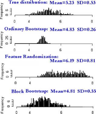
Figure 1: Comparison of different subsampling schemes.

From Figure 1, we see that block subsampling produces more reliable estimates of the variance of $S$ compared to the naive methods: ordinary bootstrapping and feature randomization. Both naive methods ignore the dependence between positions and thus fail to take into account the natural clumps of the feature II. This is the key reason for the poor performance of the two naive methods.

5.2 Simulation study IIa

Our second simulation study examines the case where the sequence is generated from a piecewise stationary model where there is more than one homogeneous region. As before, we consider the problem of estimating the percentage of base pair overlap between two features, and compare the performance of four strategies:

1. feature randomization,

2. naive block subsampling from unsegmented sequence,

3. block subsampling from sequence segmented using the true changepoints, and

4. block subsampling from sequence segmented using the changepoints estimated by the dyadic segmentation method we described in Section 4.3.

In our simulation model, we generate $X_{t}$, $Y_{t}$ independently from a Neyman–Scott process characterized as follows:

1. Cluster centers occur along the sequence according to a Poisson process of rate $\lambda_{i}$ in region $i$.

2. The number of features in each cluster follows Poisson distribution with mean $\alpha$.

3. The start of features are located at a geometric distance (mean $\mu$) from the cluster center.

4. The features are generated with length that is geometric with mean $\beta$.

5. Overlap between features generated using steps 1–4 are ignored.

For simplicity, we let there be only 2 homogeneous regions, each of length $T=10{,}000$. Consider the setting where the parameters for the two regions have the following values: $(\lambda_{1},\alpha_{1},\mu_{1},\beta_{1})=(0.01,10,10,5)$ and $(\lambda_{2},\alpha_{2},\mu_{2},\beta_{2})=(0.02,10,10,5)$. Figure 2 shows a simulated example, where features $A$ and $B$ are plotted as well as their overlap. Figure 2 also shows the cumulative sum and the segmentation. Figure 3 shows respectively the histograms of the estimated distribution of the overlap statistic $\bar{X}^{*}$ centered and scaled. It is clear that the feature randomization underestimates the standard deviation, whereas naive block subsampling without segmentation gives a mixture distribution with long tails. Strategy 3, which subsamples assuming the true changepoint at $\tau$ is known, gives the correct distribution as expected. Strategy 4, which uses the estimated changepoint, reassurringly gives a very similar distribution to strategy 3. Table 1 gives the standard deviation estimates.

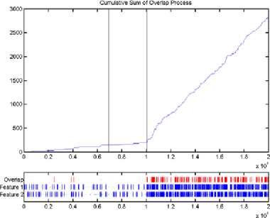
Figure 2: Example of one instance from simulation model 2. Top plot shows cumulative sum and estimated segmentation.

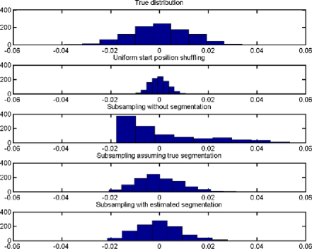
Figure 3: Comparison of different subsampling schemes.

5.3 Simulation study IIb

We utilized the Neyman–Scott process described in simulation study IIa to study the consistency of the double bootstrap method described in Section 4.4 for estimating the distribution of $R_{n}$. We consider the simple case where there is one homogeneous region. We utilized a larger region and a parameterization of the process that results in more and longer feature instances than we consider in the study above. The parameters are $T=5$ Mb and $(\lambda_{1},\alpha_{1},\mu_{1},\beta_{1})=(\lambda_{2},\alpha_{2},\mu_{2},\beta_{2})=(0.05,10,100,75)$. This yields a pair of feature-sets with around 5000 instances, where each feature-set covers around 17% of the 5 Mb region. We simulated 20,000 pairs of feature-sets from this process, and found that the mean of region-overlap between pairs, $R_{n}$, was 0.293, and the standard error was 0.0072. We subsampled 1000 sets of 10,000 draws from this distribution, each of which yielded the mean above (to 3 significant digits), and the standard errors ranged from 0.0071 to 0.0073, which corresponds almost exactly to the theoretical 95% confidence interval for the standard error of the standard error of a Gaussian with standard deviation 0.0072 after 10,000 draws. Not surprisingly, the distribution of $R_{n}$ was Gaussian, as indicated by the Lilliefors and the Shapiro–Wilk test, which did not reject the hypothesis of Gaussianity at a significance level 0.05 with the full sample of 20,000 observations.

In order to test the capacity of segmented subsampling with a version of the double block bootstrap to discover this distribution based on only a single pair of observations, we selected the most extreme pair found during simulation, for which $R_{n}$ was 0.321, corresponding to a $z$-score of 3.87. Since the number of feature instances is itself a random quantity, the job of block subsampling is particularly difficult: when $R_{n}$ is far to the right of expectation, the feature-sets tend to contain more feature instances than those closer to the center. The pair we chose was no exception. The results are given in Figure 4. Hence, it is not surprising that our subsampling procedure tends to over-estimate the mean. The Lilliefors test fails to reject the Gaussianity of any of the resulting distributions with sample sizes up to 1000 at a significance level of 0.05, but does reject it for several of the smaller block-sizes when the sample size is pushed up to 10,000. The Shapiro–Wilk test, however, detects departures from Gaussianity for many of the distributions at a significance level of 0.05 for samples larger than 500. This is because $R_{n}$ is predicated on relatively small counts of feature-instance overlaps and, hence, the distributions tend to have heavy tails.

We note that the global minimum of the Inter-Quantile (IQ) statistic was found at $L_{b}/L_{r}=0.15$ and $L_{r}/n=0.06$. That is, 0.9% of the 5 Mb region, or 45 Kb, were included in each block sample. This block sample size is certainly sufficient to capture multiple feature-clusters, since the parameterized Neyman–Scott process above yields an average inter-cluster distance of about 1 Kb.

Table 1: Estimates of standard error by four sampling strategies in simulation study IIa

	Standard error	Fold change from
Method	estimate	true value
True value	1.2e$-$002	—
Uniform shuffle	3.6e$-$003	0.30
Subsample, no segmentation	1.7e$-$002	1.40
Subsample, true segmentation	1.1e$-$002	0.91
Subsample, estimated segmentation	1.0e$-$002	0.83

Figure 4: Comparison of block subsampling distributions.

To corroborate our hypothesis that the mean was overestimated because the feature-sets we chose were more dense than most, we applied our method with learned parametrization, $L_{b}/L_{r}=0.15$ and $L_{r}/n=0.06$, for a pair of feature-sets with $R_{n}=0.293$, the population average. Indeed, the mean was estimated, after 10,000 samples, to be 0.293, and $\hat{\sigma}_{n}$ was 0.0072.

Although the purpose of this simulation was merely to check the consistency of our version of the double block bootstrap for data not unlike actual genomic data, for example, ChIP-seq “broad-peaks,” we decided to also check the performance of feature-start site shuffling for the same pair of feature-sets used above. In the case of $B_{n}$, the basepair overlap statistic, feature start-site shuffling correctly estimates the mean, but can (in the stationary case) radically underestimate the standard deviation. The same is not true in the case of $R_{n}$. Start-site shuffling is not assured (under our model) to provide an unbiased estimate of the mean or the standard deviation. We drew 10,000 samples from the distribution under shuffling, and found the mean to be 0.337, and the standard deviation to be 0.0070, which indicates that the pair of feature-sets under study in fact overlap slightly less than expected at random ($p\approx 0.011$). The fact that this conclusion is actually in the wrong direction in this relatively easy, stationary example should make us skeptical of studies that rely upon start-site shuffling to draw conclusions about statistics that cannot be defined locally, such as $R_{n}$.

Our discussion of this simulation and the following real data examples exhibit the subtleties inherent in our approach. Subtleties appear whenever inference follows regularization.

5.4 Association of noncoding ENCODE annotations and constrained sequences

Here we present a real example of the study of association between “constrained sequences” and “nonexonic annotations” from the ENCODE project, limited to the 1.87 Mbp ENCODE Pilot Region ENm001, also known as the CFTR locus. The constrained sequences are those highly conserved between human and the 14 mammalian species studied and sequenced by the ENCODE consortium. Enrichment of evolutionary constraint at the “nonexonic annotations” sites implies that the biochemical assays employed by the ENCODE consortium are capable of identifying biologically functional elements. We tested the association of noncoding annotations and constrained elements using the base pair overlap statistic $B_{n}$ in Section 4.3 using the conditional formulation. We interpret the lack of association as, given sequence composition and the distribution of each feature along the genome as observed, the assignments (by nature) of features $A$ and $B$ to individual bases are made independently. We derive the significance of the observed statistic under this null hypothesis following the method proposed in Section 4.3.

As we discussed, we have several issues to deal with:

1. [(iii)]

2. How do we segment? That is, what statistic(s) do we use for segmenation?

3. Is segmentation necessary or is the region sufficiently homogeneous?

4. If we segment, what $L_{s}$ should we use?

5. Given a segmentation, what $L_{b}$ is appropriate?

Here are our methods:

1. [(a)]

2. The simplest choice for (i) and the one we followed was to segment according to both numerator and denominator in $B_{n}$: intersect partitions and enforce an $L_{s}$ bound. Given our theory, this should ensure homogeneity in the mean of $B_{n}$.

3. Although strictly speaking (ii) and (iii) can be combined, we experimented a bit to also see if the theory of Section 4.1 was borne out in practice.

4. We did not use the $V$ statistic and thus only had to choose $L_{s}$. Again, we experimented with $L_{s}=500$ Kb to preserve as much genomic structure as possible, and $L_{s}=200$ Kb to ensure we had not undersegmented.

5. We explored a variety of values of $L_{b}$, and studied the consistency between nearby values under the interquartile statistic (IQ statistic) discussed in Section 4.6. We draw conclusions based on the value of $L_{b}$ that optimizes local consistency.

To segment the data, we applied the method in Section 4.3 to both features $A$ and $B$, or in the language of Section 4, $I$ and $J$, and then combined the segmentation. In segmenting each feature, we experimented with minimum segment lengths $L_{s}$ of 200 and 500 Kb. Before subsampling, we combined the segmentations of $A$ and $B$ by taking a union of the changepoints. This created regions with length less than $L_{s}$. However, the total length of these regions comprise $<$0.1% of the total Encode region, and were left out of the remaining analyses.

If the sequence were sufficiently homogeneous, we could forgo the initial segmentation step. Figure 5 shows an estimate of variance of $B_{n}$ (with the appropriate renormalization) for a reasonable range of $L_{b}$, both before and after segmentation. Two trends are clearly evident. First, segmentation greatly reduces the estimated variance. As we discussed in Section 4.1.2, inhomogeneity of the sequence causes an inflated estimate of variance. If the data were homogeneous, segmentation should not change the variance estimate. Thus, the fact that the estimated variances drop after segmentation for such a large range of $L_{b}$’s suggests that the data are inhomogeneous. Second, and more importantly, the estimated variance of $B_{n}$ increases sharply with increasing $L_{b}$ in the unsegmented data. This is evidence of inhomogeneity in the mean of $B_{n}$ across this ENCODE region: underlying shifts in mean, if ignored, can be mistaken for spurious long range autocorrelation, which also implicitly runs against our assumption. In either case, as Theorem 4.2 suggests, we would be overly conservative. Thus, a preliminary exploration of the data convinces us that this ENCODE region is inhomogeneous in $I$ and/or $J$ and segmentation is necessary.

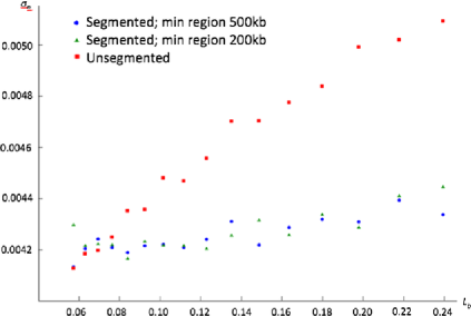
Figure 5: Estimated $\sigma_{n}$ as a function of $L_{b}$ for 10,000 samples.

We found that 200 and 500 Kb gave 5 and 3 segments respectively. Figure 6 gives the results for 500 Kb. What is fairly surprising, but reassuring, is that over the whole broad range of $L_{b}$ considered, the estimated SD of the statistic under the null was essentially flat after segmentation. Flat here means that variability was within a Monte Carlo SD for the 10,000 replications we used. We would expect longer values of $L_{b}$ to include, in our estimate of $\sigma$, additional covariance between distant genomic positions captured by the extended block-length. The fact that this, by and large, does not appear to be happening is consistent with our hypothesis that the relevant mixing distance is indeed quite small compared to the size of approximately stationary regimes.

We found that there is still moderate deviation from Gaussianity in both the segmented and unsegmented case for $0.05<L_{b}<0.25$, both in the tails, as detected by the Shapiro–Wilk test, and in the body of the distribution under the Lilliefors test. With a sample size of 100, neither test detects this departure, but at a sample size of only 500, it is detected under a number of parameterizations of $L_{b}$. As we discussed in Section 4.5, the definition of stationarity depends on the scale at which we view the genome. This suggests that our segmentation still does not take care of inhomogenity in the variance. Hence, as we have mentioned, if we use the variance for the Gaussian approximation, our results are still conservative.

The scientific conclusion of this example is that, indeed, there is strong association since the $z$-value is over 9 SDs. We note that the effect of segmentation on our scientific conclusion is essentially nonexistent. However, it is comforting to note that the change in (with and without segmentation) variance is in the correct direction.

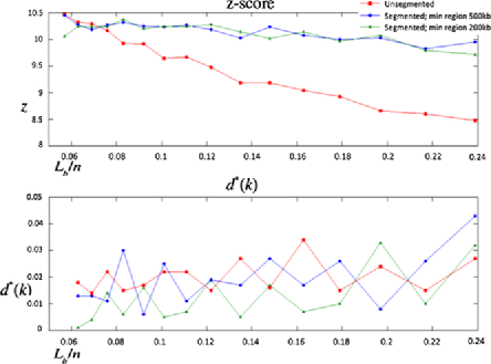
Figure 6: Comparison of block subsampling distributions, $\rho^{\beta}n$ vs. $\rho^{\beta+1}n$ under the IQR statistic. Estimates $\hat{\sigma}_{n}$ and resulting $z$-scores of $B_{n}$ shown.

5.5 The association of copy number variation with RefSeq annotated exons in the human genome

In this example, we reanalyze a published data set; this reanalysis leads to a different conclusion from the one made by the original paper. In 2006, Redon et al. published a set of 1445 genomic regions with observed Copy Number Variation (CNVs) across individuals. These regions consist of both deletions and insertions, and more than half of them overlap genes. In the paper, the authors reported, among other things, a paucity of overlap with RefSeq genes at a significance level of 0.05. The statistic that they used is precisely our marginal formulation of the region overlap statistic $R_{n}$, but the null distribution to which they referred it is quite different. Their null was computed by randomly permuting both genes and CNVs, and hence treats the entire genome (or at least entire chromosomes) as homogeneous, and the distances between feature-instances as exponential. Thus, if feature-instance lengths were all 1 bp, this would be a Poisson process. As discussed in Section 5.3, under our model this procedure provides an unbiased estimate of the mean in the case of the $B_{n}$, but is unpredictable with respect to its estimate of the variance. In the case of $R_{n}$, it is unpredictable with respect to both the mean and the variance. Here, for comparison with the result of Redon et al. (2006), we examine only $R_{n}$.

Although we have attempted to replicate this portion of the Redon study, undoubtedly there are small differences between our efforts and those of Redon et al. (2006). For instance, we have masked all genomic repeats in the “Repeat Masker” track on the UCSC genome browser (genome.ucsc.edu). Redon et al. also considered patterns of repeats in their analysis, but may have utilized an at least slightly different map of genomic repeats. We find that $61.8\%$ of the CNVs overlap RefSeq genes by at least 1 basepair. That is, we wish to assess the significance of our observed statistic $R_{n}=0.618$.

The calibration of the subsampling procedure is nontrivial, especially in this application where we must consider the additional parameter $L_{r}$. Hence, in the following we provide complete detail regarding the calibration of our method for the data of Redon et al. (2006).

As before, our analysis begins with an assessment of the need for segmentation. In this case, we are dealing with whole human chromosomes, we expect that, in general, at least some segmentation is necessary. We segmented down to a minimum segment length of 10,000,000 bps (10 Mbs), letting $L_{s}=10$ Mb. The mean length of these CNVs is around 250 Kb, and they are not uniformly distributed, so we are compelled not to segment down to regions much smaller than 10 Mb by our desire to capture the appropriate spatial distribution of clusters of feature-instances. To assess the sufficiency of the resulting segmentation, we examine the Gaussianity of the segmented subsampling distributions. This examination is tied to our selection of block length.

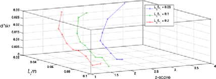
Figure 7: The relationship between the estimated $z$-score, $d^{*}(k)$, $L_{r}$ and $L_{b}$. As $L_{r}$ increases, our estimate of $\hat{\sigma}_{n}$ (not shown) increases, which drives the estimated $z$-score down. As $L_{r}$ becomes too small, we lose the stability of our estimates, and $d^{*}(k)$ increases. For the smallest value of $L_{r}$ shown here, the estimated z-score increases sharply, but the corresponding value of $d^{*}(k)$ indicates that this parameterization is unreliable. The ideal parameterization under $d^{*}(k)$ is given by $L_{r}/n=0.09$ and $L_{b}/L_{r}=0.20$.

To select an inner block length, $L_{b}$, and an outer block-length, $L_{r}$, we drew 10,000 samples for each of several lengths. We chose to use a linear, rather than exponential, scale for $L_{r}/n$: we selected 10 values from 0.01 to 0.10 in increments of 0.01. We chose three values of $L_{b}/L_{r}$, 0.05, 0.10 and 0.20. Each of these parameterizations yields several responses, including: an estimated $z$-score, $d^{*}(k)$, and measures of Gaussianity. In Figure 7, we plot the relationship between the estimated $z$-score, $d^{*}(k)$, $L_{r}$ and $L_{b}$. Regarding the Gaussianity of the resulting distributions, at a significance level of 0.01 and a sample size of 5000, neither the Shapiro–Wilk nor the Lilliefors test rejected the null hypothesis of Gaussianity for any of the 30 explored parameterizations. To supplement our biological intuition that segmentation is necessary when whole chromosomes are considered, we used the same 30 parameterizations with the unsegmented data, and performed the same tests to check the Gaussianity of the resulting distributions. Of the 30 parameterizations, 3 showed departures from Gaussianity under Lilliefors test, and 9 showed strong departures in the tails under the Shapiro–Wilks test. This indicates, as expected, that segmentation has substantially improved the Gaussianity of the sample distributions. In practice, one might attempt a finer segmentation in hopes of further reducing the (conservative) bias in $\hat{\sigma}_{n}$. For this example we are satisfied with the current segmentation.

The global minimum of $d^{*}(k)$ occurs for $L_{r}/n=0.09$ and $L_{b}/L_{r}=0.20$. This parameterization yields an estimated $z$-score of 1.25 and, therefore, we conclude that we cannot corroborate the result of Redon et al. (2006). Under our model it appears that CNVs are, if anything, very slightly positively associated with genes ($p\approx 0.105$). We note that a few parameterizations, as shown in Figure 7, do produce $z$-scores greater than 2. However, these parameterizations correspond to large values of $d^{*}(k)$ and, furthermore, significance is in the opposite direction reported by Redon et al. (2006). This highlights the need for carefully defined null distributions in genomic studies. We are not suggesting that the results presented necessarily invalidate the corresponding result of Redon et al. (2006), but rather we caution that scientific conclusions of this kind are predicated on how the researcher defines “at random,” and that this definition should be made to reflect, as much as possible, that which is known about the actual distribution of genomic elements. We presume that authors wish, in general, to err on the side of caution, and hence do not wish to report significant association when the association can be explained simply by a conservative choice of null.

[id-suppA] Some theorems in subsampling methods for genomic inference In Supplementary Material, we provide theoretical proofs to the theorems presented in the main text. [doi]10.1214/10-AOAS363SUPP [url]http://lib.stat.cmu.edu/aoas/363/supplement.pdf .pdf

References

- (1) Andrews, D. and Mallows, C. (1974). Scale mixtures of normal distributions. J. Roy. Statist. Soc. Ser. B 26 99–102. \MR0359122
- (2) Beran, R. (1988). Prepivoting test statistics: A bootstrap view of asymptotic refinements. J. Amer. Statist. Assoc. 83 687–697. \MR0963796
- (3) Bernardi, G., Olofsson, B., Filipski, J., Zerial, M., Salinas, J., Cuny, G., Meunier-Rotival, M. and Rodier, F. (1985). The mosaic genome of warm-blooded vertebrates. Science 228 953–958.
- (4) Bickel, P. J., Boley, N., Brown, J. B., Huang, H. and Zhang, N. R. (2010). Supplement to “Subsampling methods for genomic inference.” DOI: 10.1214/10-AOAS363SUPP.
- (5) Bickel, P. J. and Sakov, A. (2008). On the choice of in the out of bootstrap and its application to confidence bounds for extreme percentiles. Statist. Sinica 18 967–985. \MR2440400
- (6) Bickel, P. J., Gotze, F. and van Zwet, W. R. (1997). Resampling fewer than observations: Gains, losses, and remedies for losses. Statist. Sinica 1 1–31. \MR1441142
- (7) Birney, E. et al. (2007). Identification and analysis of functional elements in of the human genome by the ENCODE pilot project. Nature 447 799–816.
- (8) Blakesley, R. W. et al. (2004). An intermediate grade of finished genomic sequence suitable for comparative analyses. Genome Res. 14 2235–2244.
- (9) Braun, J. and Muller, H.-G. (1998). Statistical methods for DNA sequence segmentation. Statist. Sci. 13 142–162.
- (10) Carter, N. (2007). Methods and strategies for analyzing copy number variation using DNA microarrays. Nature Genet. 39 S16–S21.
- (11) Churchill, G. A. (1989). Stochastic models for heterogeneous genome sequences. Bull. Math. Biol. 51 79–94. \MR0978904
- (12) Churchill, G. A. (1992). Hidden Markov chains and the analysis of genome structure. Comput. Chem. 16 107–115.
- (13) Das, D., Banerjee, N. and Zhang, M. Q. (2004). Interacting models of cooperative gene regulation. Proc. Natl. Acad. Sci. USA 101 16234–16239.
- (14) Dedecker, J., Doukhan, P., Lang, G., Leon R., J. R., Louhichi, S. and Prieur, C. (2007). Weak Dependence: With Examples and Applications. Lecture Notes in Statist. 190. Springer, New York. \MR2338725
- (15) Efron, B. (1981). Nonparametric standard errors and confidence intervals. With discussion and a reply by the author. Canad. J. Statist. 9 139–172. \MR0640014
- (16) Fickett, J. W., Torney, D. C. and Wolf, D. R. (1992). Base compositional structure of genomes. Genomics 13 1056–1064.
- (17) Fu, Y.-X. and Curnow, R.-N. (1990). Maximum likelihood estimation of multiple change-points. Biometrika 77 563–573. \MR1087847
- (18) Gotze, F. and Rackauskas, A. (2001). Adaptive choice of bootstrap sample sizes. In State of the Art in Probability and Statistics (Leiden, 1999) 286–309. Lecture Notes Monogr. Ser. 36. Inst. Math. Statist., Beachwood, OH. \MR1836566
- (19) Gupta, M. and Liu, J. S. (2005). De novo cis-regulatory module elicitation for eukaryotic genomes. Proc. Natl. Acad. Sci. USA 102 7079–7084.
- (20) Hall, P. (1992). The Bootstrap and Edgeworth Expansion. Springer, New York. \MR1145237
- (21) Huang, H., Kao, M. C., Zhou, X., Liu, J. S. and Wong, W. H. (2004). Determination of local statistical significance of patterns in Markov sequences with application to promoter element identification. J. Comput. Biol. 11 1–14.
- (22) James, B., James, K. L. and Siegmund, D. (1987). Tests for a change-point. Biometrika 74 71–84. \MR0885920
- (23) Kato, M., Hata, N., Banerjee, N., Futcher, B. and Zhang, M. Q. (2004). Identifying combinatorial regulation of transcription factors and binding motifs. Genome Biol. 5 R56.
- (24) Künsch, H. (1989). The jackknife and the bootstrap for general stationary observations. Ann. Statist. 17 1217–1241. \MR1015147
- (25) Letson, D. and McCullough, B. D. (1998). Better confidence intervals: The double bootstrap with no pivot. Amer. J. Agr. Econ. 80 552–559.
- (26) Li, W., Stolovitzky, G., Bernaola-Galván, P. and Oliver, J. L. (1998). Compositional heterogeneity within, and uniformity between, DNA sequences of yeast chromosomes. Genome Res. 8 916–928.
- (27) Li, W., Bernaola-Galván, P., Haghighi, F. and Grosse, I. (2002). Applications of recursive segmentation to the analysis of DNA sequences. Comput. Chem. 26 491–510.
- (28) Margulies, E. H. et al. (2007). Analyses of deep mammalian sequence alignments and constraint predictions for 1% of the human genome. Genome Res. 17 760–774.
- (29) Olshen, A. B., Venkatraman, E. S., Lucito, R. and Wigler, M. (2004). Circular binary segmentation for the analysis of array-based DNA copy number data. Biostatistics 5 557–572.
- (30) Politis, D. and Romano, J. (1994). Large sample confidence regions based on subsamples under minimal assumptions. Ann. Statist. 22 2031–2050. \MR1329181
- (31) Politis, D., Romano, J. and Wolf, M. (1999). Subsampling. Springer, New York. \MR1707286
- (32) Redon, R. et al. (2006). Global variation in copy number in the human genome. Nature 444 444–454.
- (33) Thisted, R. and Efron, B. (1987). Did Shakespeare write a newly-discovered poem? Biometrika 74 445–455. \MR0909350
- (34) Venkatraman, S. (1992). Consistency results in multiple change-point problems. Ph.D. dissertation, Stanford Univ.
- (35) Vostrikova, L. J. (1981). Detecting disorder in multidimensional random process. Sov. Math. Dokl. 24 55–59.
- (36) Yu, H., Yoo, A. S. and Greenwald, I. (2004). Cluster Analyzer for Transcription Sites (CATS): A C-based program for identifying clustered transcription factor binding sites. Bioinformatics 20 1198–1200.
- (37) Zhang, C., Xuan, Z., Mandel, G. and Zhang, M. Q. (2006). A clustering property of highly-degenerate transcription factor binding sites in the mammalian genome. Nucleic Acid Res. 34 2238–2246.
- (38) Zhou, Q. and Wong, W. H. (2004). CisModule: De Novo discovery of cis-regulatory modules by hierarchical mixture modeling. Proc. Natl. Acad. Sci. USA 101 12114–12119.