Adaptive and anisotropic piecewise polynomial approximation

Abstract

We survey the main results of approximation theory for adaptive piecewise polynomial functions. In such methods, the partition on which the piecewise polynomial approximation is defined is not fixed in advance, but adapted to the given function $f$ which is approximated. We focus our discussion on (i) the properties that describe an optimal partition for $f$, (ii) the smoothness properties of $f$ that govern the rate of convergence of the approximation in the $L^{p}$-norms, and (iii) fast refinement algorithms that generate near optimal partitions. While these results constitute a fairly established theory in the univariate case and in the multivariate case when dealing with elements of isotropic shape, the approximation theory for adaptive and anisotropic elements is still building up. We put a particular emphasis on some recent results obtained in this direction.

1 Introduction

1.1 Piecewise polynomial approximation

Approximation by piecewise polynomial functions is a procedure that occurs in numerous applications. In some of them such as terrain data simplification or image compression, the function $f$ to be approximated might be fully known, while it might be only partially known or fully unknown in other applications such as denoising, statistical learning or in the finite element discretization of PDE’s. In all these applications, one usually makes the distinction between uniform and adaptive approximation. In the uniform case, the domain of interest is decomposed into a partition where all elements have comparable shape and size, while these attributes are allowed to vary strongly in the adaptive case. The partition may therefore be adapted to the local properties of $f$, with the objective of optimizing the trade-off between accuracy and complexity of the approximation. This chapter is concerned with the following fundamental questions:

• Which mathematical properties describe an optimally adapted partition for a given function $f$ ?

• For such optimally adapted partitions, what smoothness properties of $f$ govern the convergence properties of the corresponding piecewise polynomial approximations ?

• Can one construct optimally adapted partitions for a given function $f$ by a fast algorithm ?

For a given bounded domain $\Omega\subset\rm\hbox{I\kern-1.99997pt\hbox{R}}^{d}$ and a fixed integer $m>0$, we associate to any partition ${\cal T}$ of $\Omega$ the space

$$V_{\cal T}:=\{f\;\;{\rm s.t.}\;\;f_{|T}\in\rm\hbox{I\kern-1.99997pt\hbox{P}}_{m-1},\;T\in{\cal T}\}$$

of piecewise polynomial functions of total degree $m-1$ over ${\cal T}$. The dimension of this space measures the complexity of a function $g\in V_{\cal T}$. It is proportional to the cardinality of the partition:

$${\rm dim}(V_{\cal T}):=C_{m,d}\#({\cal T}),\mbox{ with }C_{m,d}:={\rm dim}(\rm\hbox{I\kern-1.99997pt\hbox{P}}_{m-1})=\binom{m+d-1}{d}.$$

In order to describe how accurately a given function $f$ may be described by piecewise polynomial functions of a prescribed complexity, it is therefore natural to introduce the error of best approximation in a given norm $\|\cdot\|_{X}$ which is defined as

$$\sigma_{N}(f)_{X}:=\inf_{\#({\cal T})\leq N}\min_{g\in V_{{\cal T}}}\|f-g\|_{X}.$$

This object of study is too vague if we do not make some basic assumptions that limitate the set of partitions which may be considered. We therefore restrict the definition of the above infimum to a class ${\cal A}_{N}$ of “admissible partitions” of complexity at most $N$. The approximation to $f$ is therefore searched in the set

$$\Sigma_{N}:=\cup_{{\cal T}\in{\cal A}_{N}}V_{{\cal T}},$$

and the error of best approximation is now defined as

$$\sigma_{N}(f)_{X}:=\inf_{g\in\Sigma_{N}}\|f-g\|_{X}=\inf_{{\cal T}\in{\cal A}_{N}}\inf_{g\in V_{\cal T}}\|f-g\|_{X}.$$

The assumptions which define the class ${\cal A}_{N}$ are usually of the following type:

1. The elementary geometry of the elements of ${\cal T}$. The typical examples that are considered in this chapter are: intervals when $d=1$, triangles or rectangles when $d=2$, simplices when $d>2$.

2. Restrictions on the regularity of the partition, in the sense of the relative size and shape of the elements that constitute the partition ${\cal T}$.

3. Restrictions on the conformity of the partition, which impose that each face of an element $T$ is common to at most one adjacent element $T^{\prime}$.

The conformity restriction is critical when imposing global continuity or higher smoothness properties in the definition of $V_{\cal T}$, and if one wants to measure the error in some smooth norm. In this survey, we limitate our interest to the approximation error measured in $X=L^{p}$. We therefore do not impose any global smoothness property on the space $V_{\cal T}$ and ignore the conformity requirement.

Throughout this chapter, we use the notation

$$e_{m,{\cal T}}(f)_{p}:=\min_{g\in V_{\cal T}}\|f-g\|_{L^{p}},$$

to denote the $L^{p}$ approximation error in the space $V_{\cal T}$ and

$$\sigma_{N}(f)_{p}:=\sigma_{N}(f)_{L^{p}}=\inf_{g\in\Sigma_{N}}\|f-g\|_{L^{p}}=\inf_{{\cal T}\in{\cal A}_{N}}e_{m,{\cal T}}(f)_{p}.$$

If $T\in{\cal T}$ is an element and $f$ is a function defined on $\Omega$, we denote by

$$e_{m,T}(f)_{p}:=\min_{\pi\in\rm\hbox{I\kern-1.39998pt\hbox{P}}_{m-1}}\|f-\pi\|_{L^{p}(T)},$$

the local approximation error. We thus have

$$e_{m,{\cal T}}(f)_{p}=\Bigl{(}\sum_{T\in{\cal T}}e_{m,T}(f)_{p}^{p}\Bigr{)}^{1/p},$$

when $p<\infty$ and

$$e_{m,{\cal T}}(f)_{\infty}=\max_{T\in{\cal T}}e_{m,T}(f)_{\infty}.$$

The norm $\|f\|_{L^{p}}$ without precision on the domain stands for $\|f\|_{L^{p}(\Omega)}$ where $\Omega$ is the full domain where $f$ is defined.

1.2 From uniform to adaptive approximation

Concerning the restrictions ont the regularity of the partitions, three situations should be distinguished:

1. Quasi-uniform partitions: all elements have approximately the same size. This may be expressed by a restriction of the type

   $$C_{1}N^{-1/d}\leq\rho_{T}\leq h_{T}\leq C_{2}N^{-1/d},$$ (1.1)

   for all $T\in{\cal T}$ with ${\cal T}\in{\cal A}_{N}$, where $0<C_{1}\leq C_{2}$ are constants independent of $N$, and where $h_{T}$ and $\rho_{T}$ respectively denote the diameters of $T$ and of it largest inscribed disc.

2. Adaptive isotropic partitions: elements may have arbitrarily different size but their aspect ratio is controlled by a restriction of the type

   $$\frac{h_{T}}{\rho_{T}}\leq C,$$ (1.2)

   for all $T\in{\cal T}$ with ${\cal T}\in{\cal A}_{N}$, where $C>1$ is independent of $N$.

3. Adaptive anisotropic partitions: element may have arbitrarily different size and aspect ratio, i.e. no restriction is made on $h_{T}$ and $\rho_{T}$.

A classical result states that if a function $f$ belongs to the Sobolev space $W^{m,p}(\Omega)$ the $L^{p}$ error of approximation by piecewise polynomial of degree $m$ on a given partition satisfies the estimate

$$e_{m,{\cal T}}(f)_{p}\leq Ch^{m}|f|_{W^{m,p}},$$ (1.3)

where $h:=\max_{T\in{\cal T}}h_{T}$ is the maximal mesh-size, $|f|_{W^{m,p}}:=\Bigl{(}\sum_{|\alpha|=m}\|\partial^{\alpha}f\|_{L^{p}}^{p}\Bigr{)}^{1/p}$ is the standard Sobolev semi-norm, and $C$ is a constant that only depends on $(m,d,p)$. In the case of quasi-uniform partitions, this yields an estimate in terms of complexity:

$$\sigma_{N}(f)_{p}\leq CN^{-m/d}|f|_{W^{m,p}},$$ (1.4)

where the constant $C$ now also depends on $C_{1}$ and $C_{2}$ in (1.1).

Here and throughout the chapter, ${\rm C}$ denotes a generic constant which may vary from one equation to the other. The dependence of this constant with respect to the relevant parameters will be mentionned when necessary.

Note that the above estimate can be achieved by restricting the family ${\cal A}_{N}$ to a single partition: for example, we start from a coarse partition ${\cal T}_{0}$ into cubes and recursively define a nested sequence of partition ${\cal T}_{j}$ by splitting each cube of ${\cal T}_{j-1}$ into $2^{d}$ cubes of half side-length. We then set

$${\cal A}_{N}:=\{{\cal T}_{j}\},\mbox{ if }\#({\cal T}_{0})2^{dj}\leq N<\#({\cal T}_{0})2^{d(j+1)}.$$

Similar uniform refinement rules can be proposed for more general partitions into triangles, simplices or rectangles. With such a choice for ${\cal A}_{N}$, the set $\Sigma_{N}$ on which one picks the approximation is thus a standard linear space. Piecewise polynomials on quasi-uniform partitions may therefore be considered as an instance of linear approximation.

The interest of adaptive partitions is that the choice of ${\cal T}\in{\cal A}_{N}$ may vary depending on $f$, so that the set $\Sigma_{N}$ is inherently a nonlinear space. Piecewise polynomials on adaptive partitions are therefore an instance of nonlinear approximation. Other instances include approximation by rational functions, or by $N$-term linear combinations of a basis or dictionary. We refer to [28] for a general survey on nonlinear approximation.

The use of adaptive partitions allows to improve significantly on (1.4). The theory that describes these improvements is rather well established for adaptive isotropic partitions: as explained further, a typical result for such partitions is of the form

$$\sigma_{N}(f)_{p}\leq CN^{-m/d}|f|_{W^{m,\tau}},$$ (1.5)

where $\tau$ can be chosen smaller than $p$. Such an estimate reveals that the same rate of decay $N^{-\frac{m}{d}}$ as in (1.4) is achieved for $f$ in a smoothness space which is larger than $W^{m,p}$. It also says that for a smooth function, the multiplicative constant governing this rate might be substantially smaller than when working with quasi-uniform partitions.

When allowing adaptive anisotropic partitions, one should expect for further improvements. From an intuitive point of view, such partitions are needed when the function $f$ itself displays locally anisotropic features such as jump discontinuities or sharp transitions along smooth manifolds. The available approximation theory for such partitions is still at its infancy. Here, typical estimates are also of the form

$$\sigma_{N}(f)_{p}\leq CN^{-m/d}A(f),$$ (1.6)

but they involve quantities $A(f)$ which are not norms or semi-norms associated with standard smoothness spaces. These quantities are highly nonlinear in $f$ in the sense that they do not satisfy $A(f+g)\leq C(A(f)+A(g))$ even with $C\geq 1$.

1.3 Outline

This chapter is organized as follows. As a starter, we study in §2 the simple case of piecewise constant approximation on an interval. This example gives a first illustration the difference between the approximation properties of uniform and adaptive partitions. It also illustrates the principle of error equidistribution which plays a crucial role in the construction of adaptive partitions which are optimally adapted to $f$. This leads us to propose and study a multiresolution greedy refinement algorithm as a design tool for such partitions. The distinction between isotropic and anisotropic partitions is irrelevant in this case, since we work with one-dimensional intervals.

We discuss in §3 the derivation of estimates of the form (1.5) for adaptive isotropic partitions. The main guiding principle for the design of the partition is again error equidistribution. Adaptive greedy refinement algorithms are discussed, similar to the one-dimensional case.

We study in §4 an elementary case of adaptive anisotropic partitions for which all elements are two-dimensional rectangles with sides that are parallel to the $x$ and $y$ axes. This type of anisotropic partitions suffer from an intrinsic lack of directional selectivity. We limitate our attention to piecewise constant functions, and identify the quantity $A(f)$ involved in (1.6) for this particular case. The main guiding principles for the design of the optimal partition are now error equidistribution combined with a local shape optimization of each element.

In §5, we present some recently available theory for piecewise polynomials on adaptive anisotropic partitions into triangles (and simplices in dimension $d>2$) which offer more directional selectivity than the previous example. We give a general formula for the quantity $A(f)$ which can be turned into an explicit expression in terms of the derivatives of $f$ in certain cases such as piecewise linear functions i.e. $m=2$. Due to the fact that $A(f)$ is not a semi-norm, the function classes defined by the finiteness of $A(f)$ are not standard smoothness spaces. We show that these classes include piecewise smooth objects separated by discontinuities or sharp transitions along smooth edges.

We present in §6 several greedy refinement algorithms which may be used to derive anisotropic partitions. The convergence analysis of these algorithms is more delicate than for their isotropic counterpart, yet some first results indicate that they tend to generate optimally adapted partitions which satisfy convergence estimates in accordance with (1.6). This behaviour is illustrated by numerical tests on two-dimensional functions.

2 Piecewise constant one-dimensional approximation

We consider here the very simple problem of approximating a continuous function by piecewise constants on the unit interval $[0,1]$, when we measure the error in the uniform norm. If $f\in C([0,1])$ and $I\subset[0,1]$ is an arbitrary interval we have

$$e_{1,I}(f)_{\infty}:=\min_{c\in\rm\hbox{I\kern-1.39998pt\hbox{R}}}\|f-c\|_{L^{\infty}(I)}=\frac{1}{2}\max_{x,y\in I}|f(x)-f(y)|.$$

The constant $c$ that achieves the minimum is the median of $f$ on $I$. Remark that we multiply this estimate at most by a factor $2$ if we take $c=f(z)$ for any $z\in I$. In particular, we may choose for $c$ the average of $f$ on $I$ which is still defined when $f$ is not continuous but simply integrable.

If ${\cal T}_{N}=\{I_{1},\cdots,I_{N}\}$ is a partition of $[0,1]$ into $N$ sub-intervals and $V_{{\cal T}_{N}}$ the corresponding space of piecewise constant functions, we thus find hat

$$e_{1,{\cal T}_{N}}(f)_{\infty}:=\min_{g\in V_{{\cal T}_{N}}}\|f-g\|_{L^{\infty}}=\frac{1}{2}\max_{k=1,\cdots,N}\max_{x,y\in I_{k}}|f(x)-f(y)|.$$ (2.7)

2.1 Uniform partitions

We first study the error of approximation when the ${\cal T}_{N}$ are uniform partitions consisting of the intervals $I_{k}=[\frac{k}{N},\frac{(k+1)}{N}]$. Assume first that $f$ is a Lipschitz function i.e. $f^{\prime}\in L^{\infty}$. We then have

$$\max_{x,y\in I_{k}}|f(x)-f(y)|\leq|I_{k}|\|f^{\prime}\|_{L^{\infty}(I_{k})}=N^{-1}\|f^{\prime}\|_{L^{\infty}}.$$

Combining this estimate with (2.7), we find that for uniform partitions,

$$f\in{\rm Lip}([0,1])\Rightarrow\sigma_{N}(f)_{\infty}\leq CN^{-1},$$ (2.8)

with $C=\frac{1}{2}\|f^{\prime}\|_{L^{\infty}}$. For less smooth functions, we may obtain lower convergence rates: if $f$ is Hölder continuous of exponent $0<\alpha<1$, we have by definition

$$|f(x)-f(y)|\leq|f|_{C^{\alpha}}|x-y|^{\alpha},$$

which yields

$$\max_{x,y\in I_{k}}|f(x)-f(y)|\leq N^{-\alpha}|f|_{C^{\alpha}}.$$

We thus find that

$$f\in C^{\alpha}([0,1])\Rightarrow\sigma_{N}(f)_{\infty}\leq CN^{-\alpha},$$ (2.9)

with $C=\frac{1}{2}|f|_{C^{\alpha}}$.

The estimates (2.8) and (2.9) are sharp in the sense that they admit a converse: it is easily checked that if $f$ is a continuous function such that $\sigma_{N}(f)_{\infty}\leq CN^{-1}$ for some $C>0$, it is necessarily Lipschitz. Indeed, for any $x$ and $y$ in $[0,1]$, consider an integer $N$ such that $\frac{1}{2}N^{-1}\leq|x-y|\leq N^{-1}$. For such an integer, there exists a $f_{N}\in V_{{\cal T}_{N}}$ such that $\|f-f_{N}\|_{L^{\infty}}\leq CN^{-1}$. We thus have

$$|f(x)-f(y)|\leq 2CN^{-1}+|f_{N}(x)-f_{N}(y)|.$$

Since $x$ and $y$ are either contained in one interval or two adjacent intervals of the partition ${\cal T}_{N}$ and since $f$ is continuous, we find that $|f_{N}(x)-f_{N}(y)|$ is either zero or less than $2CN^{-1}$. We therefore have

$$|f(x)-f(y)|\leq 4CN^{-1}\leq 8C|x-y|,$$

which shows that $f\in{\rm Lip}([0,1])$. In summary, we have the following result.

Theorem 2.1

If $f$ is a continuous function defined on $[0,1]$ and if $\sigma_{N}(f)_{\infty}$ denotes the $L^{\infty}$ error of piecewise constant approximation on uniform partitions, we have

$$f\in{\rm Lip}([0,1])\Leftrightarrow\sigma_{N}(f)_{\infty}\leq CN^{-1}.$$ (2.10)

In an exactly similar way, is can be proved that

$$f\in C^{\alpha}([0,1])\Leftrightarrow\sigma_{N}(f)_{\infty}\leq CN^{-\alpha},$$ (2.11)

These equivalences reveal that Lipschitz and Holder smoothness are the properties that do govern the rate of approximation by piecewise constant functions in the uniform norm.

The estimate (2.8) is also optimal in the sense that it describes the saturation rate of piecewise constant approximation: a higher convergence rate cannot be obtained, even for smoother functions, and the constant $C=\frac{1}{2}\|f^{\prime}\|_{L^{\infty}}$ cannot be improved. In order to see this, consider an arbitrary function $f\in C^{1}([0,1])$, so that for all $\varepsilon>0$, there exists $\eta>0$ such that

$$|x-y|\leq\eta\Rightarrow|f^{\prime}(x)-f^{\prime}(y)|\leq\varepsilon.$$

Therefore if $N$ is such that $N^{-1}\leq\eta$, we can introduce on each interval $I_{k}$ an affine function $p_{k}(x)=f(x_{k})+(x-x_{k})f^{\prime}(x_{k})$ where $x_{k}$ is an arbitrary point in $I_{k}$, and we then have

$$\|f-p_{k}\|_{L^{\infty}(I_{k})}\leq N^{-1}\varepsilon.$$

It follows that

$$\begin{array}[]{ll}e_{1,I_{k}}(f)_{\infty}&\geq e_{1,I_{k}}(p_{k})_{\infty}-e_{1,I_{k}}(f-p_{k})_{\infty}\\ &\geq e_{1,I_{k}}(p_{k})_{\infty}-\frac{1}{2}N^{-1}\varepsilon\\ &=\frac{1}{2}N^{-1}(|f^{\prime}(x_{k})|-\varepsilon),\end{array}$$

where we have used the triangle inequality

$$e_{m,T}(f+g)_{p}\leq e_{m,T}(f)_{p}+e_{m,T}(g)_{p},$$ (2.12)

Choosing for $x_{k}$ the point that maximize $|f^{\prime}|$ on $I_{k}$ and taking the supremum of the above estimate over all $k$, we obtain

$$e_{1,{\cal T}_{N}}(f)_{\infty}\geq\frac{1}{2}N^{-1}(\|f^{\prime}\|_{L^{\infty}}-\varepsilon).$$

Since $\varepsilon>0$ is arbitrary, this implies the lower estimate

$$\liminf_{N\to+\infty}\;N\sigma_{N}(f)_{\infty}\geq\frac{1}{2}\|f^{\prime}\|_{L^{\infty}}.$$ (2.13)

Combining with the upper estimate (2.8), we thus obtain the equality

$$\lim_{N\to+\infty}N\sigma_{N}(f)_{\infty}=\frac{1}{2}\|f^{\prime}\|_{L^{\infty}},$$ (2.14)

for any function $f\in C^{1}$. This identity shows that for smooth enough functions, the numerical quantity that governs the rate of convergence $N^{-1}$ of uniform piecewise constant approximations is exactly $\frac{1}{2}\|f^{\prime}\|_{L^{\infty}}$.

2.2 Adaptive partitions

We now consider an adaptive partition ${\cal T}_{N}$ for which the intervals $I_{k}$ may depend on $f$. In order to understand the gain in comparison to uniform partitions, let us consider a function $f$ such that $f^{\prime}\in L^{1}$, i.e. $f\in W^{1,1}([0,1])$. Remarking that

$$\max_{x,y\in I}|f(x)-f(y)|\leq\int_{I}|f^{\prime}(t)|dt,$$

we see that a natural choice fo the $I_{k}$ can be done by imposing that

$$\int_{I_{k}}|f^{\prime}(t)|dt=N^{-1}\int_{0}^{1}|f^{\prime}(t)|dt,$$

which means that the $L^{1}$ norm of $f^{\prime}$ is equidistributed over all intervals. Combining this estimate with (2.7), we find that for adaptive partitions,

$$f\in W^{1,1}([0,1])\Rightarrow\sigma_{N}(f)_{\infty}\leq CN^{-1},$$ (2.15)

with $C:=\frac{1}{2}\|f^{\prime}\|_{L^{1}}$. This improvement upon uniform partitions in terms of approximation properties was firstly established in [35]. The above argument may be extended to the case where $f$ belongs to the slightly larger space $BV([0,1])$ which may include discontinuous functions in contrast to $W^{1,1}([0,1])$, by asking that the $I_{k}$ are such that

$$|f|_{BV(I_{k})}\leq N^{-1}|f|_{BV}.$$

We thus have

$$f\in BV([0,1])\Rightarrow\sigma_{N}(f)_{\infty}\leq CN^{-1},$$ (2.16)

Similar to the case of uniform partitions, the estimate (2.16) is sharp in the sense that a converse result holds: if $f$ is a continuous function such that $\sigma_{N}(f)_{\infty}\leq CN^{-1}$ for some $C>0$, then it is necessarily in $BV([0,1])$. To see this, consider $N>0$ and any set of points $0\leq x_{1}<x_{2}<\cdots<x_{N}\leq 1$. We know that there exists a partition ${\cal T}_{N}$ of $N$ intervals and $f_{N}\in V_{{\cal T}_{N}}$ such that $\|f-f_{N}\|_{L^{\infty}}\leq CN^{-1}$. We define a set of points $0\leq y_{1}<y_{2}\cdots<y_{M}\leq 1$ by unioning the set of the $x_{k}$ with the nodes that define the partition ${\cal T}_{N}$, excluding $0$ and $1$, so that $M<2N$. We can write

$$\sum_{k=0}^{N-1}|f(x_{k+1})-f(x_{k})|\leq 2C+\sum_{k=0}^{N-1}|f_{N}(x_{k+1})-f_{N}(x_{k})|\leq 2C+\sum_{k=0}^{M-1}|f_{N}(y_{k+1})-f_{N}(y_{k})|.$$

Since $y_{k}$ and $y_{k+1}$ are either contained in one interval or two adjacent intervals of the partition ${\cal T}_{N}$ and since $f$ is continuous, we find that $|f_{N}(y_{k+1})-f_{N}(y_{k})|$ is either zero or less than $2CN^{-1}$, from which it follows that

$$\sum_{k=0}^{N-1}|f(x_{k+1})-f(x_{k})|\leq 6C,$$

which shows that $f$ has bounded variation. We have thus proved the following result.

Theorem 2.2

If $f$ is a continuous function defined on $[0,1]$ and if $\sigma_{N}(f)_{\infty}$ denotes the $L^{\infty}$ error of piecewise constant approximation on adaptive partitions, we have

$$f\in BV([0,1])\Leftrightarrow\sigma_{N}(f)_{\infty}\leq CN^{-1}.$$ (2.17)

In comparison with (2.8) we thus find that same rate $N^{-1}$ is governed by a weaker smoothness condition since $f^{\prime}$ is not assumed to be bounded but only a finite measure. In turn, adaptive partitions may significantly outperform uniform partition for a given function $f$: consider for instance the function $f(x)=x^{\alpha}$ for some $0<\alpha<1$. According to (2.11), the convergence rate of uniform approximation for this function is $N^{-\alpha}$. On the other hand, since $f^{\prime}(x)=\alpha x^{\alpha-1}$ is integrable, we find that the convergence rate of adaptive approximation is $N^{-1}$.

The above construction of an adaptive partition is based on equidistributing the $L^{1}$ norm of $f^{\prime}$ or the total variation of $f$ on each interval $I_{k}$. An alternative is to build ${\cal T}_{N}$ in such a way that all local errors are equal, i.e.

$$\varepsilon_{1,I_{k}}(f)_{\infty}=\eta,$$ (2.18)

for some $\eta=\eta(N)\geq 0$ independent of $k$. This new construction of ${\cal T}_{N}$ does not require that $f$ belongs to $BV([0,1])$. In the particular case where $f\in BV([0,1])$, we obtain that

$$N\eta\leq\sum_{k=1}^{N}\\ e_{1,I_{k}}(f)_{\infty}\leq\frac{1}{2}\sum_{k=1}^{N}|f|_{BV(I_{k})}\leq\frac{1}{2}|f|_{BV},$$

from which it immediately follows that

$$e_{1,{\cal T}_{N}}(f)_{\infty}=\eta\leq CN^{-1},$$

with $C=\frac{1}{2}|f|_{BV}$. We thus have obtained the same error estimate as with the previous construction of ${\cal T}_{N}$.

The basic principle of error equidistribution, which is expressed by (2.18) in the case of piecewise constant approximation in the uniform norm, plays a central role in the derivation of adaptive partitions for piecewise polynomial approximation.

Similar to the case of uniform partitions we can express the optimality of (2.15) by a lower estimate when $f$ is smooth enough. For this purpose, we make a slight restriction on the set ${\cal A}_{N}$ of admissible partitions, assuming that the diameter of all intervals decreases as $N\to+\infty$, according to

$$\max_{I_{k}\in{\cal T}_{N}}|I_{k}|\leq AN^{-1},$$

for some $A>0$ which may be arbitrarily large. Assume that $f\in C^{1}([0,1])$, so that for all $\varepsilon>0$, there exists $\eta>0$ such that

$$|x-y|\leq\eta\Rightarrow|f^{\prime}(x)-f^{\prime}(y)|\leq\frac{\varepsilon}{A}.$$ (2.19)

If $N$ is such that $AN^{-1}\leq\eta$, we can introduce on each interval $I_{k}$ an affine function $p_{k}(x)=f(x_{k})+(x-x_{k})f^{\prime}(x_{k})$ where $x_{k}$ is an arbitrary point in $I_{k}$, and we then have

$$\|f-p_{k}\|_{L^{\infty}(I_{k})}\leq N^{-1}\varepsilon.$$

It follows that

$$\begin{array}[]{ll}e_{1,I_{k}}(f)_{\infty}&\geq e_{1,I_{k}}(p_{k})_{\infty}-e_{1,I_{k}}(f-p_{k})_{\infty}\\ &\geq e_{1,I_{k}}(p_{k})_{\infty}-\frac{1}{2}N^{-1}\varepsilon\\ &=\frac{1}{2}(\int_{I_{k}}|p^{\prime}_{k}(t)|dt-N^{-1}\varepsilon)\\ &\geq\frac{1}{2}(\int_{I_{k}}|f^{\prime}(t)|dt-2N^{-1}\varepsilon).\end{array}$$

Since there exists at least one interval $I_{k}$ such that $\int_{I_{k}}|f^{\prime}(t)|dt\geq N^{-1}\|f^{\prime}\|_{L^{1}}$, it follows that

$$e_{1,{\cal T}_{N}}(f)_{\infty}\geq\frac{1}{2}N^{-1}(\|f^{\prime}\|_{L^{1}}-2\varepsilon).$$

This inequality becomes an equality only when all quantities $\int_{I_{k}}|f^{\prime}(t)|dt$ are equal, which justifies the equidistribution principle for the design of an optimal partition. Since $\varepsilon>0$ is arbitrary, we have thus obtained the lower estimate

$$\liminf_{N\to+\infty}\;N\sigma_{N}(f)\geq\frac{1}{2}\|f^{\prime}\|_{L^{1}}.$$ (2.20)

The restriction on the family of adaptive partitions ${\cal A}_{N}$ is not so severe since $A$ maybe chosen arbitrarily large. In particular, it is easy to prove that the upper estimate is almost preserved in the following sense: for a given $f\in C^{1}$ and any $\varepsilon>0$, there exists $A>0$ depending on $\varepsilon$ such that

$$\limsup_{N\to+\infty}\;N\sigma_{N}(f)\leq\frac{1}{2}\|f^{\prime}\|_{L^{1}}+\varepsilon,$$

These results show that for smooth enough functions, the numerical quantity that governs the rate of convergence $N^{-1}$ of adaptive piecewise constant approximations is exactly $\frac{1}{2}\|f^{\prime}\|_{L^{1}}$. Note that $\|f^{\prime}\|_{L^{\infty}}$ may be substantially larger than $\|f^{\prime}\|_{L^{1}}$ even for very smooth functions, in which case adaptive partitions performs at a similar rate as uniform partitions, but with a much more favorable multiplicative constant.

2.3 A greedy refinement algorithm

The principle of error distribution suggests a simple algorithm for the generation of adaptive partitions, based on a greedy refinement algorithm:

1. Initialization: ${\cal T}_{1}=\{[0,1]\}$.

2. Given ${\cal T}_{N}$ select $I_{m}\in{\cal T}_{N}$ that maximizes the local error $e_{1,I_{k}}(f)_{\infty}$.

3. Split $I_{m}$ into two sub-intervals of equal size to obtain ${\cal T}_{N+1}$ and return to step 2.

The family ${\cal A}_{N}$ of adaptive partitions that are generated by this algorithm is characterized by the restriction that all intervals are of the dyadic type $2^{-j}[n,n+1]$ for some $j\geq 0$ and $n\in\{0,\cdots,2^{j}-1\}$. We also note that all such partitions ${\cal T}_{N}$ may be identified to a finite subtree with $N$ leaves, picked within an infinite dyadic master tree ${\cal M}$ in which each node represents a dyadic interval. The root of ${\cal M}$ corresponds to $[0,1]$ and each node $I$ of generation $j$ corresponds to an interval of length $2^{-j}$ which has two children nodes of generation $j+1$ corresponding to the two halves of $I$. This identification, which is illustrated on Figure 1, is useful for coding purposes since any such subtree can be encoded by $2N$ bits.

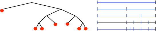
Figure 1: Adaptive dyadic partitions identify to dyadic trees

We now want to understand how the approximations generated by adaptive refinement algorithm behave in comparison to those associated with the optimal partition. In particular, do we also have that $e_{1,{\cal T}_{N}}(f)_{\infty}\leq CN^{-1}$ when $f^{\prime}\in L^{1}$ ? The answer to this question turns out to be negative, but it was proved in [30] that a slight strengthening of the smoothness assumption is sufficient to ensure this convergence rate : we instead assume that the maximal function of $f^{\prime}$ is in $L^{1}$. We recall that the maximal function of a locally integrable function $g$ is defined by

$$M_{g}(x):=\sup_{r>0}|B(x,r)|^{-1}\int_{B(x,r)}|g(t)|dt,$$

It is known that $M_{g}\in L^{p}$ if and only if $g\in L^{p}$ for $1<p<\infty$ and that $M_{g}\in L^{1}$ if and only if $g\in L\log L$, i.e. $\int_{0}^{1}|g(t)|\log(1+|g(t)|)dt<\infty$, see [42]. In this sense, the assumption that $M_{f^{\prime}}$ is integrable is only slightly stronger than $f\in W^{1,1}$.

If ${\cal T}_{N}:=(I_{1},\cdots,I_{N})$, define the accuracy

$$\eta:=\max_{1\leq k\leq N}e_{1,I_{k}}(f)_{\infty}.$$

For each $k$, we denote by $J_{k}$ the interval which is the parent of $I_{k}$ in the refinement process. From the definition of the algorithm, we necessarily have

$$\eta\leq\|f-a_{J_{k}}(f)\|_{L^{\infty}}\leq\int_{J_{k}}|f^{\prime}(t)|dt.$$

For all $x\in I_{k}$, the ball $B(x,2|I_{k}|)$ contains $J_{k}$ and it follows therefore that

$$M_{f^{\prime}}(x)\geq|B(x,2|I_{k}|)|^{-1}\int_{B(x,2|I_{k}|)}|f^{\prime}(t)|dt\geq[4|I_{k}|]^{-1}\eta,$$

which implies in turn

$$\int_{I_{k}}M_{f^{\prime}}(t)dt\geq\eta/4.$$

If $M_{f^{\prime}}$ is integrable, this yields the estimate

$$N\eta\leq 4\int_{0}^{1}M_{f^{\prime}}(t)dt.$$

It follows that

$$e_{1,{\cal T}_{N}}(f)_{\infty}=\eta\leq CN^{-1}$$

with $C=4\|M_{f^{\prime}}\|_{L^{1}}$. We have thus established the following result.

Theorem 2.3

If $f$ is a continuous function defined on $[0,1]$ and if $\sigma_{N}(f)_{\infty}$ denotes the $L^{\infty}$ error of piecewise constant approximation on adaptive partitions of dyadic type, we have

$$M_{f^{\prime}}\in L^{1}([0,1])\Rightarrow\sigma_{N}(f)_{\infty}\leq CN^{-1},$$ (2.21)

and that this rate may be achieved by the above described greedy algorithm.

Note however that a converse to (2.21) does not hold and that we do not so far know of a simple smoothness property that would be exactly equivalent to the rate of approximation $N^{-1}$ by dyadic adaptive partitions. A by-product of (2.21) is that

$$f\in W^{1,p}([0,1])\Rightarrow\sigma_{N}(f)_{\infty}\leq CN^{-1},$$ (2.22)

for any $p>1$.

3 Adaptive and isotropic approximation

We now consider the problem of piecewise polynomial approximation on a domain $\Omega\subset\rm\hbox{I\kern-1.99997pt\hbox{R}}^{d}$, using adaptive and isotropic partitions. We therefore consider a sequence $({\cal A}_{N})_{N\geq 0}$ of families of partitions that satisfies the restriction (1.2). We use piecewise polynomials of degree $m-1$ for some fixed but arbitrary $m$.

Here and in all the rest of the chapter, we restrict our attention to partitions into geometrically simple elements which are either cubes, rectangles or simplices. These simple elements satisfy a property of affine invariance: there exist a reference element $R$ such that any $T\in{\cal T}\in{\cal A}_{N}$ is the image of $R$ by an invertible affine transformation $A_{T}$. We can choose $R$ to be the unit cube $[0,1]^{d}$ or the unit simplex $\{0\leq x_{1}\leq\cdots\leq x_{d}\leq 1\}$ in the case of partitions by cubes and rectangles or simplices, respectively.

3.1 Local estimates

If $T\in{\cal T}$ is an element and $f$ is a function defined on $\Omega$, we study the local approximation error

$$e_{m,T}(f)_{p}:=\min_{\pi\in\rm\hbox{I\kern-1.39998pt\hbox{P}}_{m-1}}\|f-\pi\|_{L^{p}(T)}.$$ (3.23)

When $p=2$ the minimizing polynomial is given by

$$\pi:=P_{m,T}f,$$

where $P_{m,T}$ is the $L^{2}$-orthogonal projection, and can therefore be computed by solving a least square system. When $p\neq 2$, the minimizing polynomial is generally not easy to determine. However it is easily seen that the $L^{2}$-orthogonal projection remains an acceptable choice: indeed, it can easily be checked that the operator norm of $P_{m,T}$ in $L^{p}(T)$ is bounded by a constant $C$ that only depends on $(m,d)$ but not on the cube or simplex $T$. From this we infer that for all $f$ and $T$ one has

$$e_{m,T}(f)_{p}\leq\|f-P_{m,T}f\|_{L^{p}(T)}\leq(1+C)e_{m,T}(f)_{p}.$$ (3.24)

Local estimates for $e_{m,T}(f)_{p}$ can be obtained from local estimates on the reference element $R$, remarking that

$$e_{m,T}(f)_{p}=\Bigl{(}\frac{|T|}{|R|}\Bigr{)}^{1/p}e_{m,R}(g)_{p},$$ (3.25)

where $g=f\circ A_{T}$. Assume that $p,\tau\geq 1$ are such that $\frac{1}{\tau}=\frac{1}{p}+\frac{m}{d}$, and let $g\in W^{m,\tau}(R)$. We know from Sobolev embedding that

$$\|g\|_{L^{p}(R)}\leq C\|g\|_{W^{m,\tau}(R)},$$

where the constant $C$ depends on $p,\tau$ and $R$. Accordingly, we obtain

$$e_{m,R}(g)_{p}\leq C\min_{\pi\in\rm\hbox{I\kern-1.39998pt\hbox{P}}_{m-1}}\|g-\pi\|_{W^{m,\tau}(R)}.$$ (3.26)

We then invoke Deny-Lions theorem which states that if $R$ is a connected domain, there exists a constant $C$ that only depends on $m$ and $R$ such that

$$\min_{\pi\in\rm\hbox{I\kern-1.39998pt\hbox{P}}_{m-1}}\|g-\pi\|_{W^{m,\tau}(R)}\leq C|g|_{W^{m,\tau}(R)}.$$ (3.27)

If $g=f\circ A_{T}$, we obtain by this change of variable that

$$|g|_{W^{m,\tau}(R)}\leq C\Bigl{(}\frac{|R|}{|T|}\Bigr{)}^{1/\tau}\|B_{T}\|^{m}|f|_{W^{m,\tau}(T)},$$ (3.28)

where $B_{T}$ is the linear part of $A_{T}$ and $C$ is a constant that only depends on $m$ and $d$. A well known and easy to derive bound for $\|B_{T}\|$ is

$$\|B_{T}\|\leq\frac{h_{T}}{\rho_{R}},$$ (3.29)

Combining (3.25), (3.26), (3.27), (3.28) and (3.29), we thus obtain a local estimate of the form

$$e_{m,T}(f)_{p}\leq C|T|^{1/p-1/\tau}\,h_{T}^{m}|f|_{W^{m,\tau}(T)}=C|T|^{-m/d}h_{T}^{m}|f|_{W^{m,\tau}(T)}.$$

where we have used the relation $\frac{1}{\tau}=\frac{1}{p}+\frac{m}{d}$. From the isotropy restriction (1.2), there exists a constant $C>0$ independent of $T$ such that $h_{T}^{d}\leq C|T|$. We have thus established the following local error estimate.

Theorem 3.1

If $f\in W^{m,\tau}(\Omega)$, we have for all element $T$

$$e_{m,T}(f)_{p}\leq C|f|_{W^{m,\tau}(T)},$$ (3.30)

where the constant $C$ only depends on $m$, $R$ and the constants in (1.2).

Let us mention several useful generalizations of the local estimate (3.30) that can be obtained by a similar approach based on a change of variable on the reference element. First, if $f\in W^{s,\tau}(\Omega)$ for some $0<s\leq m$ and $\tau\geq 1$ such that $\frac{1}{\tau}=\frac{1}{p}+\frac{s}{d}$, we have

$$e_{m,T}(f)_{p}\leq C|f|_{W^{s,\tau}(T)}.$$ (3.31)

Recall that when $s$ is not an integer, the $W^{s,\tau}$ semi-norm is defined by

$$|f|_{W^{s,\tau}(\Omega)^{q}}:=\sum_{|\alpha|=n}\int_{\Omega\times\Omega}\frac{|\partial^{\alpha}f(x)-\partial^{\alpha}f(y)|^{\tau}}{|x-y|^{(s-n)\tau+d}}dxdy,$$

where $n$ is the largest integer below $s$. In the more general case where $\frac{1}{\tau}\leq\frac{1}{p}+\frac{s}{d}$, we obtain an estimate that depends on the diameter of $T$:

$$e_{m,T}(f)_{p}\leq Ch_{T}^{r}|f|_{W^{s,\tau}(T)},\;\;r:=\frac{d}{p}-\frac{d}{\tau}+s\geq 0.$$ (3.32)

Finally, remark that for a fixed $p\geq 1$ and $s$, the index $\tau$ defined by $\frac{1}{\tau}=\frac{1}{p}+\frac{s}{d}$ may be smaller than $1$, in which case the Sobolev space $W^{s,\tau}(\Omega)$ is not well defined. The local estimate remain valid if $W^{s,\tau}(\Omega)$ is replaced by the Besov space $B^{s}_{\tau,\tau}(\Omega)$. This space consists of all $f\in L^{\tau}(\Omega)$ functions such that

$$|f|_{B^{s}_{\tau,\tau}}:=\|\omega_{k}(f,\cdot)_{\tau}\|_{L^{\tau}([0,\infty[,\frac{dt}{t})},$$

is finite. Here $k$ is the smallest integer above $s$ and $\omega_{k}(f,t)_{\tau}$ denotes the $L^{\tau}$-modulus of smoothness of order $k$ defined by

$$\omega_{k}(f,t)_{\tau}:=\sup_{|h|\leq t}\|\Delta_{h}^{k}f\|_{L^{\tau}},$$

where $\Delta_{h}f:=f(\cdot+h)-f(\cdot)$ is the usual difference operator. The space $B^{s}_{\tau,\tau}$ describes functions which have “$s$ derivatives in $L^{\tau}$” in a very similar way as $W^{s,\tau}$. In particular it is known that these two spaces coincide when $\tau\geq 1$ and $s$ is not an integer. We refer to [29] and [18] for more details on Besov spaces and their characterization by approximation procedures. For all $p,\tau>0$ and $0\leq s\leq m$ such that $\frac{1}{\tau}\leq\frac{1}{p}+\frac{s}{d}$, a local estimate generalizing (3.32) has the form

$$e_{m,T}(f)_{p}\leq Ch_{T}^{r}|f|_{B^{s}_{\tau,\tau}(T)},\;\;r:=\frac{d}{p}-\frac{d}{\tau}+s\geq 0.$$ (3.33)

3.2 Global estimates

We now turn our local estimates into global estimates, recalling that

$$e_{m,{\cal T}}(f)_{p}:=\min_{g\in V_{{\cal T}}}\|f-g\|_{L^{p}}=\Bigl{(}\sum_{T\in{\cal T}}e_{m,T}(f)_{p}^{p}\Bigr{)}^{1/p};$$

with the usual modification when $p=\infty$. We apply the principle of error equidistribution assuming that the partition ${\cal T}_{N}$ is built in such way that

$$e_{m,T}(f)_{p}=\eta,$$ (3.34)

for all $T\in{\cal T}_{N}$ where $N=N(\eta)$. A first immediate estimate for the global error is therefore

$$e_{m,{\cal T}_{N}}(f)_{p}\leq N^{1/p}\eta.$$ (3.35)

Assume now that $f\in W^{m,\tau}(\Omega)$ with $\tau\geq 1$ such that $\frac{1}{\tau}=\frac{1}{p}+\frac{m}{d}$. It then follows from Theorem 3.1 that

$$N\eta^{\tau}\leq\sum_{T\in{\cal T}_{N}}e_{m,T}(f)_{p}^{\tau}\leq C\sum_{T\in{\cal T}_{N}}|f|_{W^{m,\tau}(T)}^{\tau}=C|f|_{W^{m,\tau}}^{\tau},$$

Combining with (3.35) and using the relation $\frac{1}{\tau}=\frac{1}{p}+\frac{m}{d}$, we have thus obtained that for adaptive partitions ${\cal T}_{N}$ built according to the error equidistribution, we have

$$e_{m,{\cal T}_{N}}(f)_{p}\leq CN^{-m/d}|f|_{W^{m,\tau}}.$$ (3.36)

By using (3.31), we obtain in a similar manner that if $0\leq s\leq m$ and $\tau\geq 1$ are such that $\frac{1}{\tau}=\frac{1}{p}+\frac{s}{d}$, then

$$e_{m,{\cal T}_{N}}(f)_{p}\leq CN^{-s/d}|f|_{W^{s,\tau}}.$$ (3.37)

Similar results hold when $\tau<1$ with $W^{s,\tau}$ replaced by $B^{s}_{\tau,\tau}$ but their proof requires a bit more work due to the fact that $|f|_{B^{s}_{\tau,\tau}}^{\tau}$ is not sub-additive with respect to the union of sets. We also reach similar estimate in the case $p=\infty$ by a standard modification of the argument.

The estimate (3.36) suggests that for piecewise polynomial approximation on adaptive and isotropic partitions, we have

$$\sigma_{N}(f)_{p}\leq CN^{-m/d}|f|_{W^{m,\tau}},\;\;\frac{1}{\tau}=\frac{1}{p}+\frac{m}{d}.$$ (3.38)

Such an estimate should be compared to (1.4), in a similar way as we compared (2.17) with (2.8) in the one dimensional case: the same same rate $N^{-m/d}$ is governed by a weaker smoothness condition.

In contrast to the one dimensional case, however, we cannot easily prove the validity of (3.38) since it is not obvious that there exists a partition ${\cal T}_{N}\in{\cal A}_{N}$ which equidistributes the error in the sense of (3.34). It should be remarked that the derivation of estimates such as (3.36) does not require a strict equidistribution of the error. It is for instance sufficient to assume that $e_{m,T}(f)_{p}\leq\eta$ for all $T\in{\cal T}_{N}$, and that

$$c_{1}\eta\leq e_{m,T}(f)_{p},$$

for at least $c_{2}N$ elements of ${\cal T}_{N}$, where $c_{1}$ and $c_{2}$ are fixed constants. Nevertheless, the construction of a partition ${\cal T}_{N}$ satisfying such prescriptions still appears as a difficult task both from a theoretical and algorithmical point of view.

3.3 An isotropic greedy refinement algorithm

We now discuss a simple adaptive refinement algorithm which emulates error equidistribution, similar to the algorithm which was discussed in the one dimensional case. For this purpose, we first build a hierarchy of nested quasi-uniform partitions $({\cal D}_{j})_{j\geq 0}$, where ${\cal D}_{0}$ is a coarse triangulation and where ${\cal D}_{j+1}$ is obtained from ${\cal D}_{j}$ by splitting each of its elements into a fixed number $K$ of children. We therefore have

$$\#({\cal D}_{j})=K^{j}\#({\cal D}_{0}),$$

and since the partitions ${\cal D}_{j}$ are assumed to be quasi-uniform, there exists two constants $0<c_{1}\leq c_{2}$ such that

$$c_{1}K^{-j/d}\leq h_{T}\leq c_{2}K^{-j/d},$$ (3.39)

for all $T\in{\cal D}_{j}$ and $j\geq 0$. For example, in the case of two dimensional triangulations, we may choose $K=4$ by splitting each triangle into $4$ similar triangles by the midpoint rule, or $K=2$ by bisecting each triangle from one vertex to the midpoint of the opposite edge according to a prescribed rule in order to preserve isotropy. Specific rules which have been extensively studied are bisection from the most recently generated vertex [8] or towards the longest edge [41]. In the case of partitions by rectangles, we may preserve isotropy by splitting each rectangle into $4$ similar rectangles by the midpoint rule.

The refinement algorithm reads as follows:

1. Initialization: ${\cal T}_{N_{0}}={\cal D}_{0}$ with $N_{0}:=\#({\cal D}_{0})$.

2. Given ${\cal T}_{N}$ select $T\in{\cal T}_{N}$ that maximizes $e_{m,T}(f)_{T}$.

3. Split $T$ into its $K$ childrens to obtain ${\cal T}_{N+K-1}$ and return to step 2.

Similar to the one dimensional case, the adaptive partitions that are generated by this algorithm are restricted to a particular family where each element $T$ is picked within an infinite dyadic master tree ${\cal M}=\cup_{j\geq 0}{\cal D}_{j}$ which roots are given by the elements ${\cal D}_{0}$. The partition ${\cal T}_{N}$ may be identified to a finite subtree of ${\cal M}$ with $N$ leaves. Figure 2 displays an example of adaptively refined partitions either based on longest edge bisection for triangles, or by quad-split for squares.

         

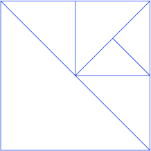
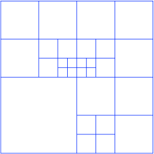
Figure 2: Adaptively refined partitions based on longest edge bisection (left) or quad-split (right)

This algorithm cannot exactly achieve error equidistribution, but our next result reveals that it generates partitions that yield error estimates almost similar to (3.36).

Theorem 3.2

If $f\in W^{m,\tau}(\Omega)$ for some $\tau\geq 1$ such that $\frac{1}{\tau}<\frac{1}{p}+\frac{m}{d}$, we then have for all $N\geq 2N_{0}=2\#({\cal D}_{0})$,

$$e_{m,{\cal T}_{N}}(f)_{p}\leq CN^{-m/d}|f|_{W^{m,\tau}},$$ (3.40)

where $C$ depends on $\tau$, $m$, $K$, $R$ and the choice of ${\cal D}_{0}$. We therefore have for piecewise polynomial approximation on adaptively refined partitions

$$\sigma_{N}(f)_{p}\leq CN^{-m/d}|f|_{W^{m,\tau}},\;\;\frac{1}{\tau}>\frac{1}{p}+\frac{m}{d}.$$ (3.41)

Proof: The technique used for proving this result is adapted from the proof of a similar result for tree-structured wavelet approximation in [19]. We define

$$\eta:=\max_{T\in{\cal T}_{N}}e_{m,T}(f)_{p},$$ (3.42)

so that we obviously have when $p<\infty$,

$$e_{m,{\cal T}_{N}}(f)_{p}\leq N^{1/p}\eta.$$ (3.43)

For $T\in{\cal T}_{N}\setminus{\cal D}_{0}$, we denote by $P(T)$ its parent in the refinement process. From the definition of the algorithm, we necessarily have

$$\eta\leq e_{m,P(T)}(f)_{p},$$

and therefore, using (3.32) with $s=m$, we obtain

$$\eta\leq Ch_{P(T)}^{r}|f|_{W^{s,\tau}(P(T))},$$ (3.44)

with $r:=\frac{d}{p}-\frac{d}{\tau}+m>0$. We next denote by ${\cal T}_{N,j}:={\cal T}_{N}\cap{\cal D}_{j}$ the elements of generation $j$ in ${\cal T}_{N}$ and define $N_{j}:=\#({\cal T}_{N,j})$. We estimate $N_{j}$ by taking the $\tau$ power of (3.44) and summing over ${\cal T}_{N,j}$ which gives

$$\begin{array}[]{ll}N_{j}\eta^{\tau}&\leq C^{\tau}\sum_{T\in{\cal T}_{N,j}}h_{P(T)}^{r\tau}|f|_{W^{s,\tau}(P(T))}^{\tau}\\ &\leq C^{\tau}(\sup_{T\in{\cal T}_{N,j}}h_{P(T)}^{r\tau})\sum_{T\in{\cal T}_{N,j}}|f|_{W^{s,\tau}(P(T))}^{\tau}\\ &\leq KC^{\tau}(\sup_{T\in{\cal D}_{j-1}}h_{T}^{r\tau})|f|_{W^{s,\tau}}^{\tau}.\end{array}$$

Using (3.39) and the fact that $\#({\cal D}_{j})=N_{0}K^{j}$, we thus obtain

$$N_{j}\leq\min\{C\eta^{-\tau}K^{-jr\tau/d}|f|_{W^{s,\tau}}^{\tau}\,,\,N_{0}K^{j}\}.$$

We now evaluate

$$N-N_{0}=\sum_{j\geq 1}N_{j}\leq\sum_{j\geq 1}\min\{C\eta^{-\tau}K^{-jr\tau/d}|f|_{W^{s,\tau}}^{\tau}\,,\,N_{0}K^{j}\}.$$

By introducing $j_{0}$ the smallest integer such that $C\eta^{-\tau}K^{-jr\tau/d}|f|_{W^{s,\tau}}^{\tau}\leq N_{0}K^{j}$, we find that

$$N-N_{0}\leq N_{0}\sum_{j\leq j_{0}}K^{j}+C\eta^{-\tau}|f|_{W^{s,\tau}}^{\tau}\sum_{j>j_{0}}K^{-jr\tau/d},$$

which after evaluation of $j_{0}$ yields

$$N-N_{0}\leq C\eta^{-\frac{d\tau}{d+r\tau}}|f|_{W^{s,\tau}}^{\frac{d\tau}{d+r\tau}}=C\eta^{-\frac{dp}{d+mp}}|f|_{W^{s,\tau}}^{\frac{dp}{d+mp}},$$

and therefore, assuming that $N\geq 2N_{0}$,

$$\eta\leq CN^{-1/p-m/d}|f|_{W^{s,\tau}}.$$

Combining this estimate with (3.43) gives the announced result. In the case $p=\infty$, a standard modification of the argument leads to a similar conclusion. $\Box$

Remark 3.3

By similar arguments, we obtain that if $f\in W^{s,\tau}(\Omega)$ for some $\tau\geq 1$ and $0\leq s\leq m$ such that $\frac{1}{\tau}<\frac{1}{p}+\frac{s}{d}$, we have

$$e_{m,{\cal T}_{N}}(f)_{p}\leq CN^{-s/d}|f|_{W^{s,\tau}}.$$

The restriction $\tau\geq 1$ may be dropped if we replace $W^{s,\tau}$ by the Besov space $B^{s}_{\tau,\tau}$, at the price of a more technical proof.

Remark 3.4

The same approximation results can be obtained if we replace $e_{m,T}(f)_{p}$ in the refinement algorithm by the more computable quantity $\|f-P_{m,T}f\|_{L^{p}(T)}$, due to the equivalence (3.24).

Remark 3.5

The greedy refinement algorithm defines a particular sequence of subtrees ${\cal T}_{N}$ of the master tree ${\cal M}$, but ${\cal T}_{N}$ is not ensured to be the best choice in the sense of minimizing the approximation error among all subtrees of cardinality at most $N$. The selection of an optimal tree can be performed by an additional pruning strategy after enough refinement has been performed. This approach was developped in the context of statistical estimation under the acronyme CART (classification and regression tree), see [12, 32]. Another approach that builds a near optimal subtree only based on refinement was proposed in [7].

Remark 3.6

The partitions which are built by the greedy refinement algorithm are non-conforming. Additional refinement steps are needed when the users insists on conformity, for instance when solving PDE’s. For specific refinement procedures, it is possible to bound the total number of elements that are due to additional conforming refinement by the total number of triangles $T$ which have been refined due to the fact that $e_{m,T}(f)_{T}$ was the largest at some stage of the algorithm, up to a fixed multiplicative constant. In turn, the convergence rate is left unchanged compared to the original non-conforming algorithm. This fact was proved in [8] for adaptive triangulations built by the rule of newest vertex bisection. A closely related concept is the amount of additional elements which are needed in order to impose that the partition satisfies a grading property, in the sense that two adjacent elements may only differ by one refinement level. For specific partitions, it was proved in [23] that this amount is bounded up to a fixed multiplicative constant the number of elements contained in the non-graded partitions. Figure 3 displays the conforming and graded partitions obtained by the minimal amount of additional refinement from the partitions of Figure 2.

         

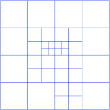
Figure 3: Conforming refinement (left) and graded refinement (right)

The refinement algorithm may also be applied to discretized data, such as numerical images. The approximated $512\times 512$ image is displayed on Figure 4 together with its approximation obtained by the refinement algorithm based on newest vertex bisection and the error measured in $L^{2}$, using $N=2000$ triangles. In this case, $f$ has the form of a discrete array of pixels, and the $L^{2}(T)$-orthogonal projection is replaced by the $\ell^{2}(S_{T})$-orthogonal projection, where $S_{T}$ is the set of pixels with centers contained in $T$. The use of adaptive isotropic partitions has strong similarity with wavelet thresholding [28, 18]. In particular, it results in ringing artifacts near the edges.

         

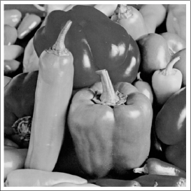
Figure 4: The image ‘peppers” (left) and its approximation by $2000$ isotropic triangles obtained by the greedy algorithm (right).

3.4 The case of smooth functions.

Although the estimate (3.38) might not be achievable for a general $f\in W^{m,\tau}(\Omega)$, we can show that for smooth enough $f$, the numerical quantity that governs the rate of convergence $N^{-\frac{n}{d}}$ is exactly $|f|_{W^{m,\tau}}:=\Bigl{(}\sum_{|\alpha|=m}\|\partial^{\alpha}f\|_{L^{\tau}}^{\tau}\Bigr{)}^{1/\tau}$ that we may define as so even for $\tau<1$. For this purpose, we assume that $f\in C^{m}(\Omega)$. Our analysis is based on the fact that such a function can be locally approximated by a polynomial of degree $m$.

We first study in more detail the approximation error on a function $q\in\rm\hbox{I\kern-1.99997pt\hbox{P}}_{m}$. We denote by ${\rm\hbox{I\kern-1.99997pt\hbox{H}}}_{m}$ the space of homogeneous polynomials of degree $m$. To $q\in\rm\hbox{I\kern-1.99997pt\hbox{P}}_{m}$, we associate its homogeneous part ${\bf q}\in{\rm\hbox{I\kern-1.99997pt\hbox{H}}}_{m}$, which is such that

$$q-{\bf q}\in\rm\hbox{I\kern-1.99997pt\hbox{P}}_{m-1}.$$

We denote by ${\bf q}_{\alpha}$ the coefficient of ${\bf q}$ associated to the multi-index $\alpha=(\alpha_{1},\cdots,\alpha_{d})$ with $|\alpha|=m$. We thus have

$$e_{m,T}(q)_{p}=e_{m,T}({\bf q})_{p}.$$

Using the affine transformation $A_{T}$ which maps the reference element $R$ onto $T$, and denoting by $B_{T}$ its linear part, we can write

$$e_{m,T}({\bf q})_{p}=\Bigl{(}\frac{|T|}{|R|}\Bigr{)}^{1/p}e_{R,m}({\bf q}\circ A_{T})_{p}=\Bigl{(}\frac{|T|}{|R|}\Bigr{)}^{1/p}e_{m,R}(\tilde{\bf q})_{p},\;\;\tilde{\bf q}:={\bf q}\circ B_{T}\in{\rm\hbox{I\kern-1.99997pt\hbox{H}}}_{m}$$

where we have used the fact that $\tilde{\bf q}-{\bf q}\circ A_{T}\in\rm\hbox{I\kern-1.99997pt\hbox{P}}_{m-1}$. Introducing for any $r>0$ the quasi-norm on ${\rm\hbox{I\kern-1.99997pt\hbox{H}}}_{m}$

$$|{\bf q}|_{r}:=\Bigl{(}\sum_{|\alpha|=m}|{\bf q}_{\alpha}|^{r}\Bigr{)}^{1/r},$$

one easily checks that

$$C^{-1}\|B_{T}^{-1}\|^{-m}|{\bf q}|_{r}\leq|\tilde{\bf q}|_{r}\leq C\|B_{T}\|^{m}|{\bf q}|_{r},$$

for some constant $C>0$ that only depends on $m$, $r$ and $R$. We then remark that $e_{R,m}({\bf q})_{p}$ is a norm on ${\rm\hbox{I\kern-1.99997pt\hbox{H}}}_{m}$, which is equivalent to $|{\bf q}|_{r}$ since ${\rm\hbox{I\kern-1.99997pt\hbox{H}}}_{m}$ is finite dimensional. It follows that there exists constants $0<C_{1}\leq C_{2}$ such that for all $q$ and $T$

$$C_{1}|T|^{1/p}\|B_{T}^{-1}\|^{-m}|{\bf q}|_{r}\leq e_{m,T}(q)_{p}\leq C_{2}|T|^{1/p}\|B_{T}\|^{m}|{\bf q}|_{r}.$$

Finally, using the bound (3.29) for $\|B_{T}\|$ and its symmetrical counterpart

$$\|B_{T}^{-1}\|\leq\frac{h_{R}}{\rho_{T}},$$

together with the isotropy restriction (1.2), we obtain with $\frac{1}{\tau}:=\frac{1}{p}+\frac{m}{d}$ the equivalence

$$C_{1}|T|^{\tau}|{\bf q}|_{r}\leq e_{m,T}(q)_{p}\leq C_{2}|T|^{\tau}|{\bf q}|_{r},$$

where $C_{1}$ and $C_{2}$ only depend on $m$, $R$ and the constant $C$ in (1.2). Choosing $r=\tau$ this equivalence can be rewritten as

$$C_{1}\Bigl{(}\sum_{|\alpha|=m}\|{\bf q}_{\alpha}\|_{L^{\tau}(T)}^{\tau}\Bigr{)}^{1/\tau}\leq e_{m,T}(q)_{p}\leq C_{2}\Bigl{(}\sum_{|\alpha|=m}\|{\bf q}_{\alpha}\|_{L^{\tau}(T)}^{\tau}\Bigr{)}^{1/\tau}.$$

Using shorter notations, this is summarized by the following result.

Lemma 3.7

Let $p\geq 1$ and $\frac{1}{\tau}:=\frac{1}{p}+\frac{m}{d}$. There exists constant $C_{1}$ and $C_{2}$ that only depends on $m$, $R$ and the constant $C$ in (1.2) such that

$$C_{1}|q|_{W^{m,\tau}(T)}\leq e_{m,T}(q)_{p}\leq C_{2}|q|_{W^{m,\tau}(T)},$$ (3.45)

for all $q\in\rm\hbox{I\kern-1.99997pt\hbox{P}}_{m}$.

In what follows, we shall frequently identify the $m$-th order derivatives of a function $f$ at some point $x$ with an homogeneous polynomial of degree $m$. In particular we write

$$|d^{m}f(x)|_{r}:=\Bigl{(}\sum_{|\alpha|=m}|\partial^{\alpha}f(x)|^{r}\Bigr{)}^{1/r}.$$

We first establish a lower estimate on $\sigma_{N}(f)$, which reflects the saturation rate $N^{-m/d}$ of the method, under a slight restriction on the set ${\cal A}_{N}$ of admissible partitions, assuming that the diameter of all elements decreases as $N\to+\infty$, according to

$$\max_{T\in{\cal T}_{N}}h_{T}\leq AN^{-1/d},$$ (3.46)

for some $A>0$ which may be arbitrarily large.

Theorem 3.8

Under the restriction (3.46), there exists a constant $c>0$ that only depends on $m$, $R$ and the constant $C$ in (1.2) such that

$$\liminf_{N\to+\infty}\;N^{m/d}\sigma_{N}(f)_{p}\geq c|f|_{W^{m,\tau}}$$ (3.47)

for all $f\in C^{m}(\Omega)$, where $\frac{1}{\tau}:=\frac{1}{p}+\frac{m}{d}$.

Proof: If $f\in C^{m}(\Omega)$ and $x\in\Omega$, we denote by $q_{x}$ the Taylor polynomial of order $m$ at the point $x=(x_{1},\cdots,x_{d})$:

$$q_{x}(y)=q_{x}(y_{1},\cdots,y_{d}):=\sum_{|\alpha|\leq m}\frac{1}{|\alpha|!}\partial^{\alpha}f(x)(y_{1}-x_{1})^{\alpha_{1}}\cdots(y_{d}-x_{d})^{\alpha_{d}}.$$ (3.48)

If ${\cal T}_{N}$ is a partition in ${\cal A}_{N}$, we may write for each element $T\in{\cal T}_{N}$ and $x\in T$

$$\begin{array}[]{ll}e_{m,T}(f)_{p}&\geq e_{m,T}(q_{x})_{p}-\|f-q_{x}\|_{L^{p}(T)}\\ &\geq C_{1}|q_{x}|_{W^{m,\tau}(T)}-\|f-q_{x}\|_{L^{p}(T)}\\ &\geq c|f|_{W^{m,\tau}(T)}-C_{1}|f-q_{x}|_{W^{m,\tau}(T)}-\|f-q_{x}\|_{L^{p}(T)},\end{array}$$

with $c:=C_{1}\min\{1,\tau\}$, where we have used the lower bound in (3.45) and the quasi-triangle inequality

$$\|u+v\|_{L^{\tau}}\leq\max\{1,\tau^{-1}\}(\|u\|_{L^{\tau}}+\|v\|_{L^{\tau}}).$$

By the continuity of the $m$-th order derivative of $f$, we are ensured that for all $\varepsilon>0$ there exists $\delta>0$ such that

$$|x-y|\leq\delta\Rightarrow|f(y)-q_{x}(y)|\leq\varepsilon|x-y|^{m}\;\;{\rm and}\;\;|d^{m}f(y)-d^{m}q_{x}|_{\tau}\leq\varepsilon.$$ (3.49)

Therefore if $N\geq N_{0}$ such that $AN_{0}^{-1/d}\leq\delta$, we have

$$\begin{array}[]{ll}e_{m,T}(f)_{p}&\geq c|f|_{W^{m,\tau}(T)}-(C_{1}\varepsilon|T|^{1/\tau}+\varepsilon h_{T}^{m}|T|^{1/p})\\ &\geq c|f|_{W^{m,\tau}(T)}-(1+C_{1})\varepsilon h_{T}^{m+d/p}\\ &\geq c|f|_{W^{m,\tau}(T)}-C\varepsilon N^{-1/\tau},\end{array}$$

where the constant $C$ depends on $C_{1}$ in (3.45) and $A$ in (3.46). Using triangle inequality, it follows that

$$e_{m,{\cal T}_{N}}(f)_{p}=\Bigl{(}\sum_{T\in{\cal T}}e_{m,T}(f)_{p}^{p}\Bigr{)}^{1/p}\geq c\Bigl{(}\sum_{T\in{\cal T}}|f|_{W^{m,\tau}(T)}^{p}\Bigr{)}^{1/p}-C\varepsilon N^{-m/d}.$$

Using Hölder’s inequality, we find that

$$|f|_{W^{m,\tau}}=\Bigl{(}\sum_{T\in{\cal T}}|f|_{W^{m,\tau}(T)}^{\tau}\Bigr{)}^{1/\tau}\leq N^{m/d}\Bigl{(}\sum_{T\in{\cal T}}|f|_{W^{m,\tau}(T)}^{p}\Bigr{)}^{1/p},$$ (3.50)

which combined with the previous estimates shows that

$$N^{m/d}e_{m,{\cal T}_{N}}(f)_{p}\geq c|f|_{W^{m,\tau}}-C\varepsilon.$$

Since $\varepsilon>0$ is arbitrary this concludes the proof. $\Box$

Remark 3.9

The Hölder’s inequality (3.50) becomes an equality if and only if all quantities in the sum are equal, which justifies the error equidistribution principle since these quantities are approximations of $e_{m,T}(f)_{p}$.

We next show that if $f\in C^{m}(\Omega)$, the adaptive approximations obtained by the greedy refinement algorithm introduced in §3.3 satisfy an upper estimate which closely matches the lower estimate (3.47).

Theorem 3.10

There exists a constant $C$ that only depends on $m$, $R$ and on the choice of the hierarchy $({\cal D}_{j})_{j\geq 0}$ such that for all $f\in C^{m}(\Omega)$, the partitions ${\cal T}_{N}$ obtained by the greedy algorithm satisfy.

$$\limsup_{N\to+\infty}\;N^{m/d}e_{m,{\cal T}_{N}}(f)_{p}\leq C|f|_{W^{m,\tau}},$$ (3.51)

where $\frac{1}{\tau}:=\frac{1}{p}+\frac{m}{d}$. In turn, for adaptively refined partitions, we have

$$\limsup_{N\to+\infty}\;N^{m/d}\sigma_{N}(f)_{p}\leq C|f|_{W^{m,\tau}},$$ (3.52)

for all $f\in C^{m}(\Omega)$.

Proof: For any $\varepsilon>0$, we choose $\delta>0$ such that (3.49) holds. We first remark that there exists $N(\delta)$ sufficiently large such that for any $N\geq N(\delta)$ at least $N/2$ elements $T\in{\cal T}_{N}$ have parents with diameter $h_{P(T)}\leq\delta$. Indeed, the uniform isotropy of the elements ensures that

$$|T|\geq ch_{P(T)}^{d},$$

for some fixed constant $c>0$. We thus have

$$\#\{T\in{\cal T}_{N}\;;\;h_{P(T)}\geq\delta\}\leq\frac{|\Omega|}{c\delta^{d}},$$

and the right-hand side is less than $N/2$ for large enough $N$. We denote by $\tilde{\cal T}_{N}$ the subset of $T\in{\cal T}_{N}$ such that $h_{P(T)}\leq\delta$. Defining $\eta$ as previously by (3.42), we observe that for all $T\in\tilde{\cal T}_{N}\setminus{\cal D}_{0}$, we have

$$\eta\leq e_{m,P(T)}(f)_{p}.$$ (3.53)

If $x$ is any point contained in $T$ and $q_{x}$ the Taylor polynomial of $f$ at this point defined by (3.48), we have

$$\begin{array}[]{ll}e_{m,P(T)}(f)_{p}&\leq e_{m,P(T)}(q_{x})_{p}+\|f-q_{x}\|_{L^{p}(P(T))}\\ &\leq C_{2}|q_{x}|_{W^{m,\tau}(P(T))}+\varepsilon h_{P(T)}^{m}|P(T)|^{1/p}\\ &\leq C_{2}\Bigl{(}\frac{|P(T)|}{|T|}\Bigr{)}^{1/\tau}|q_{x}|_{W^{m,\tau}(T)}+\varepsilon h_{P(T)}^{m}|P(T)|^{1/p}\\ &\leq C_{2}\Bigl{(}\frac{|P(T)|}{|T|}\Bigr{)}^{1/\tau}|f|_{W^{m,\tau}(T)}+\varepsilon D_{2}\Bigl{(}\frac{|P(T)|}{|T|}\Bigr{)}^{1/\tau}|T|^{1/\tau}+\varepsilon h_{P(T)}^{m}|P(T)|^{1/p},\\ \end{array}$$

where $C_{2}$ is the constant appearing in (3.45) and $D_{2}:=C_{2}\max\{1,1/\tau\}$. Combining this with (3.53), we obtain that for all $T\in\tilde{\cal T}_{N}$,

$$\eta\leq D(|f|_{W^{m,\tau}(T)}+\varepsilon|T|^{1/\tau})$$

where the constant $D$ depends on $C_{2}$, $m$ and on the refinement rule defining the hierarchy $({\cal D}_{j})_{j\geq 0}$. Elevating to the power $\tau$ and summing on all $T\in\tilde{\cal T}_{N}$, we thus obtain

$$(N/2-N_{0})\eta^{\tau}\leq\max\{1,\tau\}D^{\tau}(|f|_{W^{m,\tau}}^{\tau}+\varepsilon^{\tau}|\Omega|),$$

where $N_{0}:=\#({\cal D}_{0})$. Combining with (3.43), we therefore obtain

$$e_{m,{\cal T}_{N}}(f)_{p}\leq D\max\{\tau^{\frac{1}{\tau}},1/\tau\}N^{1/p}(N/2-N_{0})^{-1/\tau}(|f|_{W^{m,\tau}}+\varepsilon|\Omega|^{1/\tau}).$$

Taking $N>4N_{0}$ and remarking that $\varepsilon>0$ is arbitrary, we conclude that (3.52) holds with $C=4^{1/\tau}D\max\{\tau^{\frac{1}{\tau}},1/\tau\}$. $\Box$
Theorems 3.8 and 3.10 reveal that for smooth enough functions, the numerical quantity that governs the rate of convergence $N^{-m/d}$ in the $L^{p}$ norm of piecewise polynomial approximations on adaptive isotropic partitions is exactly $|f|_{W^{m,\tau}}$. In a similar way one would obtain that the same rate for quasi-uniform partitions is governed by the quantity $|f|_{W^{m,p}}$. Note however that these results are of asymptotic nature since they involve $\limsup$ and $\liminf$ as $N\to+\infty$, in contrast to Theorem 3.2. The results dealing with piecewise polynomial approximation on anisotropic adaptive partitions that we present in the next sections are of a similar asymptotic nature.

4 Anisotropic piecewise constant approximation on rectangles

We first explore a simple case of adaptive approximation on anisotropic partitions in two space dimensions. More precisely, we consider piecewise constant approximation in the $L^{p}$ norm on adaptive partitions by rectangles with sides parallel to the $x$ and $y$ axes. In order to build such partitions, $\Omega$ cannot be any polygonal domain, and for the sake of simplicity we fix it to be the unit square:

$$\Omega=[0,1]^{2}.$$

The family ${\cal A}_{N}$ consists therefore of all partitions of $\Omega$ of at most $N$ rectangles of the form

$$T=I\times J,$$

where $I$ and $J$ are intervals contained in $[0,1]$. This type of adaptive anisotropic partitions suffers from a strong coordinate bias due to the special role of the $x$ and $y$ direction: functions with sharp transitions on line edges are better approximated when these eges are parallel to the $x$ and $y$ axes. We shall remedy this defect in §5 by considering adaptive piecewise polynomial approximation on anisotropic partitions consisting of triangles, or simplices in higher dimension. Nevertheless, this first simple example is already instructive. In particular, it reveals that the numerical quantity governing the rate of approximation has an inherent non-linear structure. Throughout this section, we assume that $f$ belongs to $C^{1}([0,1]^{2})$.

4.1 A heuristic estimate

We first establish an error estimate which is based on the heuristic assumption that the partition is sufficiently fine so that we may consider that $\nabla f$ is constant on each $T$, or equivalently $f$ coincides with an affine function $q_{T}\in\rm\hbox{I\kern-1.99997pt\hbox{P}}_{1}$ on each $T$. We thus first study the local $L^{p}$ approximation error on $T=I\times J$ for an affine function of the form

$$q(x,y)=q_{0}+q_{x}x+q_{y}y.$$

Denoting by ${\bf q}(x,y):=q_{x}x+q_{y}y$ the homogeneous linear part of $q$, we first remark that

$$e_{1,T}(q)_{p}=e_{1,T}({\bf q})_{p},$$ (4.54)

since $q$ and ${\bf q}$ differ by a constant. We thus concentrate on $e_{1,T}({\bf q})_{p}$ and discuss the shape of $T$ that minimizes this error when the area $|T|=1$ is prescribed. We associate to this optimization problem a function $K_{p}$ that acts on the space of linear functions according to

$$K_{p}({\bf q})=\inf_{|T|=1}e_{1,T}({\bf q})_{p}.$$ (4.55)

As we shall explain further, the above infimum may or may not be attained.

We start by some observations that can be derived by elementary change of variable. If $a+T$ is a translation of $T$, then

$$e_{1,a+T}({\bf q})_{p}=e_{1,T}({\bf q})_{p}$$ (4.56)

since ${\bf q}$ and ${\bf q}(\cdot-a)$ differ by a constant. Therefore, if $T$ is a minimizing rectangle in (4.55), then $a+T$ is also one. If $hT$ is a dilation of $T$, then

$$e_{1,hT}({\bf q})_{p}=h^{2/p+1}e_{1,T}({\bf q})_{p}$$ (4.57)

Therefore, if we are interested in minimizing the error for an area $|T|=A$, we find that

$$\inf_{|T|=A}e_{1,T}(q)_{p}=A^{1/\tau}K_{p}({\bf q}),\;\;\frac{1}{\tau}:=\frac{1}{p}+\frac{1}{2}$$ (4.58)

and the minimizing rectangles for (4.58) are obtained by rescaling the minimizing rectangles for (4.55).

In order to compute $K_{p}({\bf q})$, we thus consider a rectangle $T=I\times J$ of unit area which barycenter is the origin. In the case $p=\infty$, using the notation $X:=|q_{x}|\,|I|/2$ and $Y:=|q_{y}|\,|J|/2$, we obtain

$$e_{1,T}({\bf q})_{\infty}=X+Y.$$

We are thus interested in the minimization of the function $X+Y$ under the constraint $XY=|q_{x}q_{y}|/4$. Elementary computations show that when $q_{x}q_{y}\neq 0$, the infimum is attained when $X=Y=\frac{1}{2}\sqrt{|q_{y}q_{x}|}$ which yields

$$|I|=\sqrt{\frac{|q_{y}|}{|q_{x}|}}\;\;{\rm and}\;\;|J|=\sqrt{\frac{|q_{x}|}{|q_{y}|}}.$$

Note that the optimal aspect ratio is given by the simple relation

$$\frac{|I|}{|J|}=\frac{|q_{y}|}{|q_{x}|},$$ (4.59)

which expresses the intuitive fact that the refinement should be more pronounced in the direction where the function varies the most. Computing $e_{1,T}(q)_{\infty}$ for such an optimized rectangle, we find that

$$K_{\infty}({\bf q})=\sqrt{|q_{y}q_{x}|}.$$ (4.60)

In the case $p=2$, we find that

$$\begin{array}[]{ll}e_{1,T}({\bf q})_{2}^{2}&=\int_{-|I|/2}^{|I|/2}\int_{-|J|/2}^{|J|/2}|q_{x}x+q_{y}y|^{2}dy\,dx\\ &=\int_{-|I|/2}^{|I|/2}\int_{-|J|/2}^{|J|/2}(q_{x}^{2}x^{2}+q_{y}^{2}y^{2}+2q_{x}q_{y}xy)dy\,dx\\ &=4\int_{0}^{|I|/2}\int_{0}^{|J|/2}(q_{x}^{2}x^{2}+q_{y}^{2}y^{2})dy\,dx\\ &=\frac{4}{3}(q_{x}^{2}(|I|/2)^{3}|J|/2+q_{y}^{2}(|J|/2)^{3}|I|/2)\\ &=\frac{1}{3}(X^{2}+Y^{2}),\end{array}$$

where we have used the fact that $|I|\,|J|=1$. We now want to minimize the function $X^{2}+Y^{2}$ under the constraint $XY=|q_{x}q_{y}|/4$. Elementary computations again show that when $q_{x}q_{y}\neq 0$, the infimum is again attained when $X=Y=\frac{1}{2}\sqrt{|q_{y}q_{x}|}$, and therefore leads to the same aspect ratio given by (4.59), and the value

$$K_{2}({\bf q})=\frac{1}{\sqrt{6}}\sqrt{|q_{x}q_{y}|}.$$ (4.61)

For other values of $p$ the computation of $e_{1,T}({\bf q})_{p}$ is more tedious, but leads to a same conclusion: the optimal aspect ratio is given by (4.59) and the function $K_{p}$ has the general form

$$K_{p}({\bf q})=C_{p}\sqrt{|q_{x}q_{y}|},$$ (4.62)

with $C_{p}:=\Bigl{(}\frac{2}{(p+1)(p+2)}\Bigr{)}^{1/p}$. Note that the optimal shape of $T$ does not depend on the $L^{p}$ metric in which we measure the error.

By (4.54), (4.56) and (4.57), we find that for shape-optimized triangles of arbitrary area, the error is given by

$$e_{1,T}(q)_{p}=|T|^{1/\tau}K_{p}({\bf q})_{p}=C_{p}\sqrt{|q_{y}q_{x}|}|T|^{1/\tau},$$ (4.63)

Note that $C_{p}$ is uniformly bounded for all $p\geq 1$.

In the case where $q\neq 0$ but $q_{x}q_{y}=0$, the infimum in (4.55) is not attained, and the rectangles of a minimizing sequence tend to become infinitely long in the direction where $q$ is constant. We ignore at the moment this degenerate case.

Since we have assumed that $f$ coincides with an affine function on $T$, the estimate (4.63) yields

$$e_{1,T}(f)_{p}=C_{p}\left\|\sqrt{|\partial_{x}f\partial_{y}f|}\right\|_{L^{\tau}(T)}=\|K_{p}(\nabla f)\|_{L^{\tau}},\;\;\frac{1}{\tau}:=\frac{1}{p}+\frac{1}{2}.$$ (4.64)

where we have identifed $\nabla f$ to the linear function $(x,y)\mapsto x\partial_{x}f+y\partial_{y}f$. This local estimate should be compared to those which were discussed in §3.1 for isotropic elements: in the bidimensional case, the estimate (3.30) of Theorem 3.1 can be restated as

$$e_{1,T}(f)_{p}\leq C\|\nabla f\|_{L^{\tau}(T)},\;\;\frac{1}{\tau}:=\frac{1}{p}+\frac{1}{2}.$$

The improvement in (4.64) comes the fact that $\sqrt{|\partial_{x}f\partial_{y}f|}$ may be substantially smaller than $|\nabla f|$ when $|\partial_{x}f|$ and $|\partial_{y}f|$ have different order of magnitude which reflects an anisotropic behaviour for the $x$ and $y$ directions. However, let us keep in mind that the validity of (4.64) is only when $f$ is identified to an affine function on $T$.

Assume now that the partition ${\cal T}_{N}$ is built in such a way that all rectangles have optimal shape in the above described sense, and obeys in addition the error equidistribution principle, which by (4.64) means that

$$\|K_{p}(\nabla f)\|_{L^{\tau}(T)}=\eta,\;\;T\in{\cal T}_{N}.$$

Then, we have on the one hand that

$$e_{1,{\cal T}_{N}}(f)_{p}\leq\eta N^{1/p},$$

and on the other hand, that

$$N\eta^{\tau}\leq\|K_{p}(\nabla f)\|_{L^{\tau}}^{\tau}.$$

Combining the two above, and using the relation $\frac{1}{\tau}:=\frac{1}{p}+\frac{1}{2}$, we thus obtain the error estimate

$$\sigma_{N}(f)_{p}\leq N^{-1/2}\|K_{p}(\nabla f)\|_{L^{\tau}}.$$ (4.65)

This estimate should be compared with those which were discussed in §3.2 for adaptive partition with isotropic elements: for piecewise constant functions on adaptive isotropic partitions in the two dimensional case, the estimate (3.38) can be restated as

$$\sigma_{N}(f)_{p}\leq CN^{-1/2}\|\nabla f\|_{L^{\tau}},\;\;\frac{1}{\tau}=\frac{1}{p}+\frac{1}{2}.$$

As already observed for local estimates, the improvement in (4.64) comes from the fact that $|\nabla f|$ is replaced by the possibly much smaller $\sqrt{|\partial_{x}f\partial_{y}f|}$. It is interesting to note that the quantity

$$A_{p}(f):=\|K_{p}(\nabla f)\|_{L^{\tau}}=C_{p}\left\|\sqrt{|\partial_{x}f\partial_{y}f|}\right\|_{L^{\tau}},$$

is strongly nonlinear in the sense that it does not satisfy for any $f$ and $g$ an inequality of the type $A_{p}(f+g)\leq C(A_{p}(f)+A_{p}(g))$, even with $C>1$. This reflects the fact that two functions $f$ and $g$ may be well approximated by piecewise constants on anisotropic rectangular partitions while their sum $f+g$ may not be.

4.2 A rigourous estimate

We have used heuristic arguments to derive the estimate (4.65), and a simple example shows that this estimate cannot hold as such: if $f$ is a non-constant function that only depends on the variable $x$ or $y$, the quantity $A_{p}(f)$ vanishes while the error $\sigma_{N}(f)_{p}$ may be non-zero. In this section, we prove a valid estimate by a rigourous derivation. The price to pay is in the asymptotic nature of the new estimate, which has a form similar to those obtained in §3.4.

We first introduce a “tamed” variant of the function $K_{p}$, in which we restrict the search of the infimum to rectangles of limited diameter. For $M>0$, we define

$$K_{p,M}({\bf q})=\min_{|T|=1,h_{T}\leq M}e_{1,T}({\bf q})_{p}.$$ (4.66)

In contrast to the definition of $K_{p}$, the above minimum is always attained, due to the compactness in the Hausdorff distance of the set of rectangles of area $1$, diameter less or equal to $M$, and centered at the origin. It is also not difficult to check that the functions ${\bf q}\mapsto e_{1,T}({\bf q})_{p}$ are uniformly Lipschitz continuous for all $T$ of area $1$ and diameter less than $M$: there exists a constant $C_{M}$ such that

$$|e_{1,T}({\bf q})_{p}-e_{1,T}(\tilde{\bf q})_{p}|\leq C_{M}|{\bf q}-\tilde{\bf q}|,$$ (4.67)

where $|{\bf q}|:=(q_{x}^{2}+q_{y}^{2})^{1/2}$. In turn $K_{p,M}$ is also Lipschitz continuous with constant $C_{M}$. Finally, it is obvious that $K_{p,M}({\bf q})\to K_{p}({\bf q})$ as $M\to+\infty$.

If $f$ is a $C^{1}$ function, we denote by

$$\omega(\delta):=\max_{|z-z^{\prime}|\leq\delta}|\nabla f(z)-\nabla f(z^{\prime})|,$$

the modulus of continuity of $\nabla f$, which satisfies $\lim_{\delta\to 0}\omega(\delta)=0$. We also define for all $z\in\Omega$

$$q_{z}(z^{\prime})=f(z)+\nabla f\cdot(z^{\prime}-z),$$

the Taylor polynomial of order $1$ at $z$. We identify its linear part to the gradient of $f$ at $z$:

$${\bf q}_{z}=\nabla f(z).$$

We thus have

$$|f(z^{\prime})-q_{z}(z^{\prime})|\leq|z-z^{\prime}|\omega(|z-z^{\prime}|).$$

At each point $z$, we denote by $T_{M}(z)$ a rectangle of area $1$ which is shape-optimized with respect to the gradient of $f$ at $z$ in the sense that it solves (4.66) with ${\bf q}={\bf q}_{z}$. The following results gives an estimate of the local error for $f$ for such optimized triangles.

Lemma 4.1

Let $T=a+hT_{M}(z)$ be a rescaled and shifted version of $T_{M}(z)$. We then have for any $z^{\prime}\in T$

$$e_{1,T}(f)_{p}\leq(K_{p,M}({\bf q}_{z^{\prime}})+B_{M}\omega(\max\{|z-z^{\prime}|,h_{T}\}))|T|^{1/\tau},$$

with $B_{M}:=2C_{M}+M$.

Proof: For all $z,z^{\prime}\in\Omega$, we have

$$\begin{array}[]{ll}e_{1,T_{M}}({\bf q}_{z^{\prime}})&\leq e_{1,T_{M}}({\bf q}_{z})+C_{M}|{\bf q}_{z}-{\bf q}_{z^{\prime}}|\\ &=K_{p,M}({\bf q}_{z})+C_{M}|{\bf q}_{z}-{\bf q}_{z^{\prime}}|\\ &\leq K_{p,M}({\bf q}_{z^{\prime}})+2C_{M}|{\bf q}_{z}-{\bf q}_{z^{\prime}}|\\ &\leq K_{p,M}({\bf q}_{z^{\prime}})+2C_{M}\omega(|z-z^{\prime}|).\end{array}$$

We then observe that if $z^{\prime}\in T$

$$\begin{array}[]{ll}e_{1,T}(f)_{p}&\leq e_{1,T}({\bf q}_{z^{\prime}})+\|f-q_{z^{\prime}}\|_{L^{p}(T)}\\ &\leq e_{1,T_{M}}({\bf q}_{z^{\prime}})|T|^{1/\tau}+\|f-q_{z^{\prime}}\|_{L^{\infty}(T)}|T|^{1/p}\\ &\leq(K_{p,M}({\bf q}_{z^{\prime}})+2C_{M}\omega(|z-z^{\prime}|))|T|^{1/\tau}+h_{T}\omega(h_{T})|T|^{1/p}\\ &\leq(K_{p,M}({\bf q}_{z^{\prime}})+2C_{M}\omega(|z-z^{\prime}|)+M\omega(h_{T}))|T|^{1/\tau},\end{array}$$

which concludes the proof. $\Box$  
We are now ready to state our main convergence theorem.

Theorem 4.2

For piecewise constant approximation on adaptive anisotropic partitions on rectangles, we have

$$\limsup_{N\to+\infty}\;N^{1/2}\sigma_{N}(f)_{p}\leq\|K_{p}(\nabla f)\|_{L^{\tau}}.$$ (4.68)

for all $f\in C^{1}([0,1]^{2})$.

Proof: We first fix some number $\delta>0$ and $M>0$ that are later pushed towards $0$ and $+\infty$ respectively. We define a uniform partition ${\cal T}_{\delta}$ of $[0,1]$ into squares $S$ of diameter $h_{S}\leq\delta$, for example by $j_{0}$ iterations of uniform dyadic refinement, where $j_{0}$ is chosen large enough such that $2^{-j_{0}+1/2}\leq\delta$. We then build partitions ${\cal T}_{N}$ by further decomposing the square elements of ${\cal T}_{\delta}$ in an anisotropic way. For each $S\in{\cal T}_{\delta}$, we pick an arbitrary point $z_{S}\in S$ (for example the barycenter of $S$) and consider the Taylor polynomial $q_{z_{S}}$ of degree $1$ of $f$ at this point. We denote by $T_{S}=T_{M}({\bf q}_{z_{S}})$ the rectangle of area $1$ such that,

$$e_{1,T_{S}}({\bf q}_{z_{S}})_{p}=\min_{|T|=1,h_{T}\leq M}e_{1,T}({\bf q}_{z_{S}})_{p}=K_{p,M}({\bf q}_{z_{S}}).$$

For $h>0$, we rescale this rectangle according to

$$T_{h,S}=h(K_{p,M}({\bf q}_{z_{S}})+(B_{M}+C_{M})\omega(\delta)+\delta)^{-\tau/2}T_{S}.$$

and we define ${\cal T}_{h,S}$ as the tiling of the plane by $T_{h,S}$ and its translates. We assume that $hC_{A}\leq\delta$ so that $h_{T}\leq\delta$ for all $T\in{\cal T}_{h,S}$ and all $S$. Finally, we define the partition

$${\cal T}_{N}=\{T\cap S\,;\;T\in{\cal T}_{h,S}\;{\rm and}\;S\in{\cal T}_{\delta}\}.$$

We first estimate the local approximation error. By lemma (4.1), we obtain that for all $T\in{\cal T}_{h,S}$ and $z^{\prime}\in T\cap S$

$$\begin{array}[]{ll}e_{1,T\cap S}(f)_{p}&\leq e_{1,T}(f)_{p}\\ &\leq(K_{p,M}({\bf q}_{z^{\prime}})+B_{M}\omega(\delta))|T|^{1/\tau}\\ &\leq h^{2/\tau}(K_{p,M}({\bf q}_{z_{S}})+(B_{M}+C_{M})\omega(\delta))(K_{p,M}({\bf q}_{z_{S}})+(B_{M}+C_{M})\omega(\delta)+\delta)^{-1}\\ &\leq h^{2/\tau}\end{array}$$

The rescaling has therefore the effect of equidistributing the error on all rectangles of ${\cal T}_{N}$, and the global approximation error is bounded by

$$e_{1,{\cal T}_{N}}(f)_{p}\leq N^{1/p}h^{2/\tau}$$ (4.69)

We next estimate the number of rectangles $N=\#({\cal T}_{N})$, which behaves like

$$\begin{array}[]{ll}N&=(1+\eta(h))\sum_{S\in{\cal T}_{\delta}}\frac{|S|}{|T_{h,S}|}\\ &=(1+\eta(h))h^{-2}\sum_{S\in{\cal T}_{\delta}}|S|(K_{p,M}({\bf q}_{z_{S}})+(B_{M}+C_{M})\omega(\delta)+\delta)^{\tau}\\ &=(1+\eta(h))h^{-2}\sum_{S\in{\cal T}_{\delta}}\int_{S}(K_{p,M}({\bf q}_{z_{S}})+(B_{M}+C_{M})\omega(\delta)+\delta)^{\tau},\end{array}$$

where $\eta(h)\to 0$ as $h\to 0$. Recalling that $K_{p,M}({\bf q}_{z_{S}})$ is Lipschitz continuous with constant $C_{M}$, it follows that

$$N\leq(1+\eta(h))h^{-2}\int_{\Omega}(K_{p,M}({\bf q}_{z})+(B_{M}+2C_{M})\omega(\delta)+\delta)^{\tau}.$$ (4.70)

Combining (4.69) and (4.70), we have thus obtained

$$N^{1/2}e_{1,{\cal T}_{N}}(f)_{p}\leq(1+\eta(h))^{1/\tau}\|K_{p,M}({\bf q}_{z})+(B_{M}+2C_{M})\omega(\delta)+\delta\|_{L^{\tau}}.$$

Observing that for all $\varepsilon>0$, we can choose $M$ large enough and $\delta$ and $h$ small enough so that

$$(1+\eta(h))^{1/\tau}\|K_{p,M}({\bf q}_{z})+(B_{M}+2C_{M})\omega(\delta)+\delta\|_{L^{\tau}}\leq\|K_{p,M}({\bf q}_{z})\|_{L^{\tau}}+\varepsilon,$$

this concludes the proof. $\Box$  
In a similar way as in Theorem 3.8, we can establish a lower estimate on $\sigma_{N}(f)$, which reflects the saturation rate $N^{-1/2}$ of the method, and shows that the numerical quantity that governs this rate is exactly equal to $\|K_{p}(\nabla f)\|_{L^{\tau}}$. We again impose a slight restriction on the set ${\cal A}_{N}$ of admissible partitions, assuming that the diameter of all elements decreases as $N\to+\infty$, according to

$$\max_{T\in{\cal T}_{N}}h_{T}\leq AN^{-1/2},$$ (4.71)

for some $A>0$ which may be arbitrarily large.

Theorem 4.3

Under the restriction (4.71), we have

$$\liminf_{N\to+\infty}\;N^{1/2}\sigma_{N}(f)_{p}\geq\|K_{p}(\nabla f)\|_{L^{\tau}}$$ (4.72)

for all $f\in C^{1}(\Omega)$, where $\frac{1}{\tau}:=\frac{1}{p}+\frac{1}{2}$.

Proof: We assume here $p<\infty$. The case $p=\infty$ can be treated by a simple modification of the argument. Here, we need a lower estimate for the local approximation error, which is a counterpart to Lemma 4.1. We start by remarking that for all rectangle $T\in\Omega$ and $z\in T$, we have

$$|e_{1,T}(f)_{p}-e_{1,T}(q_{z})_{p}|\leq\|f-q_{z}\|_{L^{p}(T)}\leq|T|^{1/p}h_{T}\omega(h_{T}),$$

and therefore

$$e_{1,T}(f)_{p}\geq e_{1,T}(q_{z})_{p}-|T|^{1/p}h_{T}\omega(h_{T})\geq K_{p}({\bf q}_{z})|T|^{1/\tau}-|T|^{1/p}h_{T}\omega(h_{T})$$

Then, using the fact that if $(a,b,c)$ are positive numbers such that $a\geq b-c$ one has $a^{p}\geq b^{p}-pcb^{p-1}$, we find that

$$\begin{array}[]{ll}e_{1,T}(f)_{p}^{p}&\geq K_{p}({\bf q}_{z})^{p}|T|^{p/\tau}-pK_{p}({\bf q}_{z})^{p-1}|T|^{(p-1)/\tau}|T|^{1/p}h_{T}\omega(h_{T})\\ &=K_{p}({\bf q}_{z})^{p}|T|^{1+p/2}-pK_{p}({\bf q}_{z})^{p-1}|T|^{1+(p-1)/2}h_{T}\omega(h_{T}),\end{array}$$

Defining $C:=p\max_{z\in\Omega}K_{p}({\bf q}_{z})^{p-1}$ and remarking that $|T|^{(p-1)/2}\leq h^{p-1}$, this leads to the estimate

$$e_{1,T}(f)_{p}^{p}\geq K_{p}({\bf q}_{z})^{p}|T|^{1+p/2}-Ch_{T}^{p}|T|\omega(h_{T}).$$

Since we work under the assumption (4.71), we can rewrite this estimate as

$$e_{1,T}(f)_{p}^{p}\geq K_{p}({\bf q}_{z})^{p}|T|^{1+p/2}-C|T|N^{-p/2}\varepsilon(N),$$ (4.73)

where $\varepsilon(N)\to 0$ as $N\to\infty$. Integrating (4.73) over $T$, gives

$$e_{1,T}(f)_{p}^{p}\geq\int_{T}(K_{p}({\bf q}_{z})^{p}|T|^{p/2}-CN^{-p/2}\varepsilon(N))dz.$$

Summing over all rectangles $T\in{\cal T}_{N}$ and denoting by $T_{z}$ the triangle that contains $z$, we thus obtain

$$e_{1,{\cal T}_{N}}(f)_{p}^{p}\geq\int_{\Omega}K_{p}(\nabla f(z))^{p}|T_{z}|^{p/2}dz-C|\Omega|N^{-p/2}\varepsilon(N).$$ (4.74)

Using Hölder inequality, we find that

$$\int_{\Omega}K_{p}(\nabla f(z))^{\tau}dz\leq\Bigl{(}\int_{\Omega}K_{p}(\nabla f(z))^{p}|T_{z}|^{p/2}dz\Bigr{)}^{\tau/p}\Bigl{(}\int_{\Omega}|T_{z}|^{-1}dz\Bigr{)}^{1-\tau/p}.$$ (4.75)

Since $\int_{\Omega}|T_{z}|^{-1}dz=\#({\cal T}_{N})=N$, it follows that

$$e_{1,{\cal T}_{N}}(f)_{p}^{p}\geq\|K_{p}(\nabla f)\|_{L^{\tau}}^{p}N^{-p/2}-C|\Omega|N^{-p/2}\varepsilon(N),$$

which concludes the proof. $\Box$

Remark 4.4

The Hölder inequality (4.75) which is used in the above proof becomes an equality when the quantity $K_{p}(\nabla f(z))^{p}|T_{z}|^{p/2}$ and $|T_{z}|^{-1}$ are proportional, i.e. $K_{p}(\nabla f(z))|T|^{1/\tau}$ is constant, which again reflects the principle of error equidistribution. In summary, the optimal partitions should combine this principe with locally optimized shapes for each element.

5 Anisotropic piecewise polynomial approximation

We turn to adaptive piecewise polynomial approximation on anisotropic partitions consisting of triangles, or simplices in higher dimension. Here $\Omega\subset\mathbb{R}^{d}$ is a domain that can be decomposed into such partitions, therefore a polygon when $d=2$, a polyhedron when $d=3$, etc. The family ${\cal A}_{N}$ consists therefore of all partitions of $\Omega$ of at most $N$ simplices. The first estimates of the form (1.6) were rigorously established in [17] and [5] in the case of piecewise linear element for bidimensional triangulations. Generalization to higher polynomial degree as well as higher dimensions were recently proposed in [14, 15, 16] as well as in [39]. Here we follow the general approach of [39] to the characterization of optimal partitions.

5.1 The shape function

If $f$ belongs to $C^{m}(\Omega)$, where $m-1$ is the degree of the piecewise polynomials that we use for approximation, we mimic the heuristic approach proposed for piecewise constants on rectangles in §4.1 by assuming that on each triangle $T$ the relative variation of $d^{m}f$ is small so that it can be considered as a constant over $T$. This means that $f$ is locally identified with its Taylor polynomial of degree $m$ at $z$, which is defined as

$$q_{z}(z^{\prime}):=f(z)+\nabla f(z)\cdot(z^{\prime}-z)+\sum_{k=2}^{m}\frac{1}{k!}d^{k}f(z)[z^{\prime}-z,\cdots,z^{\prime}-z].$$

If $q\in\rm\hbox{I\kern-1.99997pt\hbox{P}}_{m}$ is a polynomial of degree $m$, we denote by ${\bf q}\in\rm\hbox{I\kern-1.99997pt\hbox{H}}^{m}$ its homogeneous part of degree $m$. For $q=q_{z}$ we can identify ${\bf q}_{z}\in\rm\hbox{I\kern-1.99997pt\hbox{H}}_{m}$ with $\frac{1}{m!}d^{m}f(z)$. Since ${\bf q}-q\in\rm\hbox{I\kern-1.99997pt\hbox{P}}_{m-1}$ we have

$$e_{m,T}(q)_{p}=e_{m,T}({\bf q})_{p}.$$

We optimize the shape of the simplex $T$ with respect to ${\bf q}$ by introducing the function $K_{m,p}$ defined on the space $\rm\hbox{I\kern-1.99997pt\hbox{H}}_{m}$

$$K_{m,p}({\bf q}):=\inf_{|T|=1}e_{m,T}({\bf q})_{p},$$ (5.76)

where the infimum is taken among all triangles of area $1$. This infimum may or may not be attained. We refer to $K_{m,p}$ as the shape function. It is obviously a generalization of the function $K_{p}$ introduced for piecewise constant on rectangles in §4.1.

As in the case of rectangles, some elementary properties of $K_{m,p}$ are obtained by change of variable: if $a+T$ is a shifted version of $T$, then

$$e_{m,a+T}({\bf q})_{p}=e_{m,T}({\bf q})_{p}$$ (5.77)

since ${\bf q}$ and ${\bf q}(\cdot-a)$ differ by a polynomial of degree $m-1$, and that if $hT$ is a dilation of $T$, then

$$e_{m,hT}({\bf q})_{p}=h^{d/p+m}e_{m,T}({\bf q})_{p}$$ (5.78)

Therefore, if $T$ is a minimizing simplex in (5.76), then $a+T$ is also one, and if we are interested in minimizing the error for a given area $|T|=A$, we find that

$$\inf_{|T|=A}e_{m,T}(q)_{p}=A^{1/\tau}K_{m,p}({\bf q}),\;\;\frac{1}{\tau}:=\frac{1}{p}+\frac{m}{d}$$ (5.79)

and the minimizing simplex for (4.58) are obtained by rescaling the minimizing simplex for (4.55).

Remarking in addition that if $\varphi$ is an invertible linear transform, we then have for all $f$

$$|{\rm det}(\varphi)|^{1/p}e_{m,T}(f\circ\varphi)_{p}=e_{m,\varphi(T)}(f)_{p},$$

and using (5.79), we also obtain that

$$K_{m,p}({\bf q}\circ\varphi)=|{\rm det}(\varphi)|^{m}K_{m,p}({\bf q})$$ (5.80)

The minimizing simplex of area $1$ for ${\bf q}\circ\varphi$ is obtained by application of $\varphi^{-1}$ followed by a rescaling by $|{\rm det}(\varphi)|^{1/d}$ to the minimizing simplex of area $1$ for ${\bf q}$ if it exists.

5.2 Algebraic expressions of the shape function

The identity (5.80) can be used to derive the explicit expression of $K_{m,p}$ for particular values of $(m,p,d)$, as well as the exact shape of the minimizing triangle $T$ in (5.76).

We first consider the case of piecewise affine elements on two dimensional triangulations, which corresponds to $d=m=2$. Here ${\bf q}$ is a quadratic form and we denote by $\det({\bf q})$ its determinant. We also denote by $|{\bf q}|$ the positive quadratic form associated with the absolute value of the symmetric matrix associated to ${\bf q}$.

If ${\rm det}({\bf q})\neq 0$, there exists a $\varphi$ such that ${\bf q}\circ\varphi$ is either $x^{2}+y^{2}$ or $x^{2}-y^{2}$, up to a sign change, and we have $|{\rm det}({\bf q})|=|{\rm det}(\varphi)|^{-2}$. It follows from (5.80) that $K_{2,p}({\bf q})$ has the simple form

$$K_{2,p}({\bf q})=\kappa_{p}|{\rm det}({\bf q})|^{1/2},$$ (5.81)

where $\kappa_{p}:=K_{2,p}(x^{2}+y^{2})$ if ${\rm det}({\bf q})>0$ and $\kappa_{p}=K_{2,p}(x^{2}-y^{2})$ if ${\rm det}({\bf q})<0$.

The triangle of area $1$ that minimizes the $L^{p}$ error when ${\bf q}=x^{2}+y^{2}$ is the equilateral triangle, which is unique up to rotations. For ${\bf q}=x^{2}-y^{2}$, the triangle that minimizes the $L^{p}$ error is unique up to an hyperbolic transformation with eigenvalues $t$ and $1/t$ and eigenvectors $(1,1)$ and $(1,-1)$ for any $t\neq 0$. Therefore, such triangles may be highly anisotropic, but at least one of them is isotropic. For example, it can be checked that a triangle of area $1$ that minimizes the $L^{\infty}$ error is given by the half square with vertices $((0,0),(\sqrt{2},0),(0,\sqrt{2}))$. It can also be checked that an equilateral triangle $T$ of area $1$ is a “near-minimizer” in the sense that

$$e_{2,T}({\bf q})_{p}\leq CK_{2,p}({\bf q}),$$

where $C$ is a constant independent of $p$. It follows that when ${\rm det}({\bf q})\neq 0$, the triangles which are isotropic with respect to the distorted metric induced by $|{\bf q}|$ are “optimally adapted” to ${\bf q}$ in the sense that they nearly minimize the $L^{p}$ error among all triangles of similar area.

In the case when ${\rm det}({\bf q})=0$, which corresponds to one-dimensional quadratic forms ${\bf q}=(ax+by)^{2}$, the minimum in (5.76) is not attained and the minimizing triangles become infinitely long along the null cone of ${\bf q}$. In that case one has $K_{2,p}({\bf q})=0$ and the equality (5.81) remains therefore valid.

These results easily generalize to piecewise affine functions on simplicial partitions in higher dimension $d>1$: one obtains

$$K_{2,p}({\bf q})=\kappa_{p}|{\rm det}({\bf q})|^{1/d},$$ (5.82)

where $\kappa_{p}$ only takes a finite number of possible values. When ${\rm det}({\bf q})\neq 0$, the simplices which are isotropic with respect to the distorted metric induced by $|{\bf q}|$ are “optimally adapted” to ${\bf q}$ in the sense that they nearly minimize the $L^{p}$ error among all simplices of similar volume.

The analysis becomes more delicate for higher polynomial degree $m\geq 3$. For piecewise quadratic elements in dimension two, which corresponds to $m=3$ and $d=2$, it is proved in [39] that

$$K_{3,p}({\bf q})=\kappa_{p}|{\rm disc}({\bf q})|^{1/4}.$$

for any homogeneous polynomial ${\bf q}\in\rm\hbox{I\kern-1.99997pt\hbox{H}}_{3}$, where

$${\rm disc}(ax^{3}+bx^{2}y+cxy^{2}+dy^{3}):=b^{2}c^{2}-4ac^{3}-4b^{3}d+18abcd-27a^{2}d^{2},$$

is the usual discriminant and $\kappa_{p}$ only takes two values depending on the sign of ${\rm disc}({\bf q})$. The analysis that leads to this result also describes the shape of the triangles which are optimally adapted to ${\bf q}$.

For other values of $m$ and $d$, the exact expression of $K_{m,p}({\bf q})$ is unknown, but it is possible to give equivalent versions in terms of polynomials $Q_{m,d}$ in the coefficients of ${\bf q}$, in the following sense: for all ${\bf q}\in\rm\hbox{I\kern-1.99997pt\hbox{H}}_{m}$

$$c_{1}(Q_{m,d}({\bf q}))^{\frac{1}{r}}\leq K_{3,p}({\bf q})\leq c_{2}(Q_{m,d}({\bf q}))^{\frac{1}{r}},$$

where $r:={\rm deg}(Q_{m,d})$, see [39].

Remark 5.1

It is easily checked that the shape functions ${\bf q}\mapsto K_{m,p}({\bf q})$ are equivalent for all $p$ $p$ in the sense that there exist constant $0<C_{1}\leq C_{2}$ that only depend on the dimension $d$ such that

$$C_{1}K_{m,\infty}({\bf q})\leq K_{m,p}({\bf q})\leq C_{2}K_{m,\infty}({\bf q}),$$

for all ${\bf q}\in\rm\hbox{I\kern-1.99997pt\hbox{H}}_{m}$ and $p\geq 1$. In particular a minimizing triangle for $K_{m,\infty}$ is a near-minimizing triangle for $K_{m,p}$. In that sense, the optimal shape of the element does not strongly depend on $p$.

5.3 Error estimates

Following at first a similar heuristics as in §4.1 for piecewise constants on rectangles, we assume that the triangulation ${\cal T}_{N}$ is such that all its triangles $T$ have optimized shape with respect to the polynomial $q$ that coincides with $f$ on $T$.

According to (5.79), we thus have for any triangle $T\in{\cal T}$,

$$e_{m,T}(f)_{p}=|T|^{\frac{1}{\tau}}K_{m,p}({\bf q})=\left\|K_{m,p}\Bigl{(}\frac{d^{m}f}{m!}\Bigr{)}\right\|_{L^{\tau}(T)}.$$

We then apply the principle of error equidistribution, assuming that

$$e_{m,T}(f)_{p}=\eta,$$

From which it follows that $e_{m,{\cal T}_{N}}(f)_{p}\leq N^{1/p}\eta$ and

$$N\eta^{\tau}\leq\left\|K_{m,p}\Bigl{(}\frac{d^{m}f}{m!}\Bigr{)}\right\|_{L^{\tau}}^{\tau},$$

and therefore

$$\sigma_{N}(f)_{p}\leq N^{-m/d}\left\|K_{m,p}\Bigl{(}\frac{d^{m}f}{m!}\Bigr{)}\right\|_{L^{\tau}}.$$ (5.83)

This estimate should be compared to (3.38) which was obtained for adaptive partitions with elements of isotropic shape. The essential difference is in the quantity $K_{m,p}\Bigl{(}\frac{d^{m}f}{m!}\Bigr{)}$ which replaces $d^{m}f$ in the $L^{\tau}$ norm, and which may be significantly smaller. Consider for example the case of piecewise affine elements, for which we can combine (5.83) with (5.82) to obtain

$$\sigma_{N}(f)_{p}\leq CN^{-2/d}\left\||{\rm det}(d^{2}f)|^{1/d}\right\|_{L^{\tau}}.$$ (5.84)

In comparison to (3.38), the norm of the hessian $|d^{2}f|$ is replaced by the quantity $|{\rm det}(d^{2}f)|^{1/d}$ which is geometric mean of its eigenvalues, a quantity which is significantly smaller when two eigenvalues have different orders of magnitude which reflects an anisotropic behaviour in $f$.

As in the case of piecewise constants on rectangles, the example of a function $f$ depending on only one variable shows that the estimate (5.84) cannot hold as such. We may obtain some valid estimates by following the same approach as in Theorem 4.2. This leads to the following result which is established in [39].

Theorem 5.2

For piecewise polynomial approximation on adaptive anisotropic partitions into simplices, we have

$$\limsup_{N\to+\infty}\;N^{m/d}\sigma_{N}(f)_{p}\leq C\left\|K_{m,p}\Bigl{(}\frac{d^{m}f}{m!}\Bigr{)}\right\|_{L^{\tau}},\;\;\frac{1}{\tau}:=\frac{1}{p}+\frac{m}{d},$$ (5.85)

for all $f\in C^{m}(\Omega)$. The constant $C$ can be chosen equal to $1$ in the case of two-dimensional triangulations $d=2$.

The proof of this theorem follows exactly the same line as the one of Theorem 4.2: we build a sequence of partitions ${\cal T}_{N}$ by refining the triangles $S$ of a sufficiently fine quasi-uniform partition ${\cal T}_{\delta}$, intersecting each $S$ with a partition ${\cal T}_{h,S}$ by elements with shape optimally adapted to the local value of $d^{m}f$ on each $S$. The constant $C$ can be chosen equal to $1$ in the two-dimensional case, due to the fact that it is then possible to build ${\cal T}_{h,S}$ as a tiling of triangles which are all optimally adapted. This is no longer possible in higher dimension, which explains the presence of a constant $C=C(m,d)$ larger than $1$.

We may also obtain lower estimates, following the same approach as in Theorem 4.3: we first impose a slight restriction on the set ${\cal A}_{N}$ of admissible partitions, assuming that the diameter of the elements decreases as $N\to+\infty$, according to

$$\max_{T\in{\cal T}_{N}}h_{T}\leq AN^{-1/d},$$ (5.86)

for some $A>0$ which may be arbitrarily large. We then obtain the following result, which proof is similar to the one of Theorem 4.3.

Theorem 5.3

Under the restriction (5.86), we have

$$\liminf_{N\to+\infty}\;N^{m/d}\sigma_{N}(f)_{p}\geq\left\|K_{m,p}\Bigl{(}\frac{d^{m}f}{m!}\Bigr{)}\right\|_{L^{\tau}}$$ (5.87)

for all $f\in C^{m}(\Omega)$, where $\frac{1}{\tau}:=\frac{1}{p}+\frac{m}{d}$.

5.4 Anisotropic smoothness and cartoon functions

Theorem 5.2 reveals an improvement over the approximation results based on adaptive isotropic partitions in the sense that $\|K_{m,p}\Bigl{(}\frac{d^{m}f}{m!}\Bigr{)}\|_{L^{\tau}}$ may be significantly smaller than $\|d^{m}f\|_{L^{\tau}}$, for functions which have an anisotropic behaviour. However, this result suffers from two major defects:

1. The estimate (5.85) is asymptotic: it says that for all $\varepsilon>0$, there exists $N_{0}$ depending on $f$ and $\varepsilon$ such that

   $$\sigma_{N}(f)_{p}\leq CN^{-m/d}\Bigl{(}\left\|K_{m,p}\Bigl{(}\frac{d^{m}f}{m!}\Bigr{)}\right\|_{L^{\tau}}+\varepsilon\Bigr{)},$$

   for all $N\geq N_{0}$. However, it does not ensure a uniform bound on $N_{0}$ which may be very large for certain $f$.

2. Theorem 5.2 is based on the assumption $f\in C^{m}(\Omega)$, and therefore the estimate (5.85) only seems to apply to sufficiently smooth functions. This is in contrast to the estimates that we have obtained for adaptive isotropic partitions, which are based on the assumption that $f\in W^{m,\tau}(\Omega)$ or $f\in B^{m}_{\tau,\tau}(\Omega)$.

The first defect is due to the fact that a certain amount of refinement should be performed before the relative variation of $d^{m}f$ is sufficiently small so that there is no ambiguity in defining the optimal shape of the simplices. It is in that sense unavoidable.

The second defect raises a legitimate question concerning the validity of the convergence estimate (5.85) for functions which are not in $C^{m}(\Omega)$. It suggests in particular to introduce a class of distributions such that

$$\left\|K_{m,p}\Bigl{(}\frac{d^{m}f}{m!}\Bigr{)}\right\|_{L^{\tau}}<+\infty,$$

and to try to understand if the estimate remains valid inside this class which describe in some sense functions which have a certain amount anisotropic smoothness. The main difficulty is that that this class is not well defined due to the nonlinear nature of $K_{m,p}\Bigl{(}\frac{d^{m}f}{m!}\Bigr{)}$. As an example consider the case of piecewise linear elements on two dimensional triangulation, that corresponds to $m=d=2$. In this case, we have seen that $K_{2,p}({\bf q})=\kappa_{p}\sqrt{|{\rm det}({\bf q})|}$. The numerical quantity that governs the approximation rate $N^{-1}$ is thus

$$A_{p}(f):=\left\|\sqrt{|{\rm det}(d^{2}f)|}\right\|_{L^{\tau}},\;\;\frac{1}{\tau}=\frac{1}{p}+1.$$

However, this quantity cannot be defined in the distribution sense since the product of two distributions is generally ill-defined. On the other hand, it is known that the rate $N^{-1}$ can be achieved for functions which do not have $C^{2}$ smoothness, and which may even be discontinuous along curved edges. Specifically, we say that $f$ is a cartoon function on $\Omega$ if it is almost everywhere of the form

$$f=\sum_{1\leq i\leq k}f_{i}\raise 1.29167pt\hbox{\large$\chi$}_{\Omega_{i}},$$

where the $\Omega_{i}$ are disjoint open sets with piecewise $C^{2}$ boundary, no cusps (i.e. satisfying an interior and exterior cone condition), and such that $\overline{\Omega}=\cup_{i=1}^{k}\overline{\Omega}_{i}$, and where for each $1\leq i\leq k$, the function $f_{i}$ is $C^{2}$ on a neighbourhood of $\overline{\Omega}_{i}$. Such functions are a natural candidates to represent images with sharp edges or solutions of PDE’s with shock profiles.

Let us consider a fixed cartoon function $f$ on a polygonal domain $\Omega$ associated with a partition $(\Omega_{i})_{1\leq i\leq k}$. We define

$$\Gamma:=\bigcup_{1\leq i\leq k}\partial\Omega_{i},$$

the union of the boundaries of the $\Omega_{i}$. The above definition implies that $\Gamma$ is the disjoint union of a finite set of points ${\cal P}$ and a finite number of open curves $(\Gamma_{i})_{1\leq i\leq l}$.

$$\Gamma=\Bigl{(}\bigcup_{1\leq i\leq l}\Gamma_{i}\Bigr{)}\cup{\cal P}.$$

If we consider the approximation of $f$ by piecewise affine function on a triangulation ${\cal T}_{N}$ of cardinality $N$, we may distinguish two types of elements of ${\cal T}_{N}$. A triangle $T\in{\cal T}_{N}$ is called “regular” if $T\cap\Gamma=\emptyset$, and we denote the set of such triangles by ${\cal T}_{N}^{r}$. Other triangles are called “edgy” and their set is denoted by ${\cal T}_{N}^{e}$. We can thus split $\Omega$ according to

$$\Omega:=(\cup_{T\in{\cal T}_{N}^{r}}T)\cup(\cup_{T\in{\cal T}_{N}^{e}}T)=\Omega_{N}^{r}\cup\Omega_{N}^{e}.$$

We split accordingly the $L^{p}$ approximation error into

$$e_{2,{\cal T}_{N}}(f)_{p}^{p}=\sum_{T\in{\cal T}_{N}^{r}}e_{2,T}(f)_{p}^{p}+\sum_{T\in{\cal T}_{N}^{e}}e_{2,T}(f)_{p}^{p}.$$

We may use $\mathcal{O}(N)$ triangles in ${\cal T}_{N}^{e}$ and ${\cal T}_{N}^{r}$ (for example $N/2$ in each set). Since $f$ has discontinuities along $\Gamma$, the approximation error on the edgy triangles does not tend to zero in $L^{\infty}$ and ${\cal T}_{N}^{e}$ should be chosen so that $\Omega_{N}^{e}$ has the aspect of a thin layer around $\Gamma$. Since $\Gamma$ is a finite union of $C^{2}$ curves, we can build this layer of width $\mathcal{O}(N^{-2})$ and therefore of global area $|\Omega_{N}^{e}|\leq CN^{-2}$, by choosing long and thin triangles in ${\cal T}_{N}^{e}$. On the other hand, since $f$ is uniformly $C^{2}$ on $\Omega_{N}^{r}$, we may choose all triangles in ${\cal T}_{N}^{r}$ of regular shape and diameter $h_{T}\leq CN^{-1/2}$. Hence we obtain the following heuristic error estimate, for a well designed anisotropic triangulation:

$$\begin{array}[]{ll}e_{2,{\cal T}_{N}}(f)_{p}&\leq\sum_{T\in{\cal T}_{N}^{r}}|T|e_{2,T}(f)_{\infty}^{p}+\sum_{T\in{\cal T}_{N}^{e}}|T|e_{2,T}(f)_{\infty}^{p}\\ &\leq C|\Omega_{N}^{r}|(\sup_{T\in{\cal T}_{N}^{r}}h_{T}^{2})\|d^{2}f\|_{L^{\infty}(\Omega_{N}^{r})}^{p}+C|\Omega_{N}^{e}|\|f\|_{L^{\infty}(\Omega_{N}^{e})}^{p},\end{array}$$

and therefore

$$e_{2,{\cal T}_{N}}(f)_{p}\leq CN^{-\min\{1,2/p\}},$$ (5.88)

where the constant $C$ depends on $\|d^{2}f\|_{L^{\infty}(\Omega\setminus\Gamma)}$, $\|f\|_{L^{\infty}(\Omega)}$ and on the number, length and maximal curvature of the $C^{2}$ curves which constitute $\Gamma$.

These heuristic estimates have been discussed in [38] and rigorously proved in [25]. Observe in particular that the error is dominated by the edge contribution when $p>2$ and by the smooth contribution when $p<2$. For the critical value $p=2$ the two contributions have the same order.

For $p\geq 2$, we obtain the approximation rate $N^{-1}$ which suggests that approximation results such as Theorem 5.2 should also apply to cartoon functions and that the quantity $A_{p}(f)$ should be finite for such functions. In some sense, we want to “bridge the gap” between results of anisotropic piecewise polynomial approximation for cartoon functions and for smooth functions. For this purpose, we first need to give a proper meaning to $A_{p}(f)$ when $f$ is a cartoon function. As already explained, this is not straightforward, due to the fact that the product of two distributions has no meaning in general. Therefore, we cannot define $\det(d^{2}f)$ in the distribution sense, when the coefficients of $d^{2}f$ are distributions without sufficient smoothness.

We describe a solution to this problem proposed in [22] which is based on a regularization process. In the following, we consider a fixed radial nonnegative function $\varphi$ of unit integral and supported in the unit ball, and define for all $\delta>0$ and $f$ defined on $\Omega$,

$$\varphi_{\delta}(z):=\frac{1}{\delta^{2}}\varphi\left(\frac{z}{\delta}\right)\text{ and }f_{\delta}=f*\varphi_{\delta}.$$ (5.89)

It is then possible to gives a meaning to $A_{p}(f)$ based on this regularization. This approach is additionally justified by the fact that sharp curves of discontinuity are a mathematical idealisation. In real world applications, such as photography, several physical limitations (depth of field, optical blurring) impose a certain level of blur on the edges.

If $f$ is a cartoon function on a set $\Omega$, and if $x\in\Gamma\setminus{\cal P}$, we denote by $[f](x)$ the jump of $f$ at this point. We also denote by $|\kappa(x)|$ the absolute value of the curvature at $x$. For $p\in[1,\infty]$ and $\tau$ defined by $\frac{1}{\tau}:=1+\frac{1}{p}$, we introduce the two quantities

$$S_{p}(f) := \left\|\sqrt{|\det(d^{2}f)|}\right\|_{L^{\tau}(\Omega\setminus\Gamma)}=A_{p}(f_{|\Omega\setminus\Gamma}),$$

$$E_{p}(f) := \|\sqrt{|\kappa|}[f]\|_{L^{\tau}(\Gamma)},$$

which respectively measure the “smooth part” and the “edge part” of $f$. We also introduce the constant

$$C_{p,\varphi}:=\|\sqrt{|\Phi\Phi^{\prime}|}\|_{L^{\tau}(\mathbb{R})},\;\;\Phi(x):=\int_{y\in\mathbb{R}}\varphi(x,y)dy.$$ (5.90)

Note that $f_{\delta}$ is only properly defined on the set

$$\Omega^{\delta}:=\{z\in\Omega\;;\;B(z,\delta)\subset\Omega\},$$

and therefore, we define $A_{p}(f_{\delta})$ as the $L^{\tau}$ norm of $\sqrt{|\det(d^{2}f_{\delta})|}$ on this set. The following result is proved in [22].

Theorem 5.4

For all cartoon functions $f$, the quantity $A_{p}(f_{\delta})$ behaves as follows:

• If $p<2$, then

  $$\lim_{\delta\to 0}A_{p}(f_{\delta})=S_{p}(f).$$

• If $p=2$, then $\tau=\frac{2}{3}$ and

  $$\lim_{\delta\to 0}A_{2}(f_{\delta})=(S_{2}(f)^{\tau}+E_{2}(f)^{\tau}C_{2,\varphi}^{\tau})^{1/\tau}.$$

• If $p>2$, then $A_{p}(f_{\delta})\to\infty$ according to

  $$\lim_{\delta\to 0}\delta^{\frac{1}{2}-\frac{1}{p}}A_{p}(f_{\delta})=E_{p}(f)C_{p,\varphi}.$$

Remark 5.5

This theorem reveals that as $\delta\to 0$, the contribution of the neighbourhood of $\Gamma$ to $A_{p}(f_{\delta})$ is neglectible when $p<2$ and dominant when $p>2$, which was already remarked in the heuristic computation leading to (5.88).

Remark 5.6

In the case $p=2$, it is interesting to compare the limit expression $(S_{2}(f)^{\tau}+E_{2}(f)^{\tau}C_{2,\varphi}^{\tau})^{1/\tau}$ with the total variation $TV(f)=|f|_{BV}$. For a cartoon function, the total variation also can be split into a contribution of the smooth part and a contribution of the edge, according to

$$TV(f):=\int_{\Omega\setminus\Gamma}|\nabla f|+\int_{\Gamma}|[f]|.$$

Functions of bounded variation are thus allowed to have jump discontinuities along edges of finite length. For this reason, $BV$ is frequently used as a natural smoothness space to describe the mathematical properties of images. It is also well known that $BV$ is a regularity space for certain hyperbolic conservation law, in the sense that the total variation of their solutions remains finite for all time $t>0$. In recent years, it has been observed that the space $BV$ (and more generally classical smoothness spaces) do not provide a fully satisfactory description of piecewise smooth functions arising in the above mentionned applications, in the sense that the total variation only takes into account the size of the sets of discontinuities and not their geometric smoothness. In contrast, we observe that the term $E_{2}(f)$ incorporates an information on the smoothness of $\Gamma$ through the presence of the curvature $|\kappa|$. The quantity $A_{2}(f)$ appears therefore as a potential substitute to $TV(f)$ in order to take into account the geometric smoothness of the edges in cartoon function and images.

6 Anisotropic greedy refinement algorithms

In the two previous sections, we have established error estimates in $L^{p}$ norms for the approximation of a function $f$ by piecewise polynomials on optimally adapted anisotropic partitions. Our analysis reveals that the optimal partition needs to satisfy two intuitively desirable features:

1. Equidistribution of the local error.

2. Optimal shape adaptation of each element based on the local properties of $f$.

For instance, in the case of piecewise affine approximation on triangulations, these items mean that each triangle $T$ should be close to equilateral with respect to a distorted metric induced by the local value of the hessian $d^{2}f$.

From the computational viewpoint, a commonly used strategy for designing an optimal triangulation consists therefore in evaluating the hessian $d^{2}f$ and imposing that each triangle is isotropic with respect to a metric which is properly related to its local value. We refer in particular to [10] and to [9] where this program is executed by different approaches, both based on Delaunay mesh generation techniques (see also the software package [45] which includes this type of mesh generator). While these algorithms produce anisotropic meshes which are naturally adapted to the approximated function, they suffer from two intrinsic limitations:

1. They are based on the data of $d^{2}f$, and therefore do not apply well to non-smooth or noisy functions.

2. They are non-hierarchical: for $N>M$, the triangulation ${\cal T}_{N}$ is not a refinement of ${\cal T}_{M}$.

Similar remark apply to anisotropic mesh generation techniques in higher dimensions or for finite elements of higher degree.

The need for hierarchical partitions is critical in the construction of wavelet bases, which play an important role in applications to image and terrain data processing, in particular data compression [19]. In such applications, the multilevel structure is also of key use for the fast encoding of the information. Hierarchy is also useful in the design of optimally converging adaptive methods for PDE’s [8, 40, 43]. However, all these developments are so far mostly limited to isotropic refinement methods, in the spirit of the refinement procedures discussed in §3. Let us mention that hierarchical and anisotropic triangulations have been investigated in [36], yet in this work the triangulations are fixed in advance and therefore generally not adapted to the approximated function.

A natural objective is therefore to design adaptive algorithmic techniques that combine hierarchy and anisotropy, that apply to any function $f\in L^{p}(\Omega)$, and that lead to optimally adapted partitions.

In this section, we discuss anisotropic refinement algorithms which fullfill this objective. These algorithms have been introduced and studied in [20] for piecewise polynomial approximation on two-dimensional triangulations. In the particular case of piecewise affine elements, it was proved in [21] that they lead to optimal error estimates. The main idea is again to refine the element $T$ that maximizes the local error $e_{m,T}(f)_{p}$, but to allow several scenarios of refinement for this element. Here are two typical instances in two dimensions:

1. For rectangular partitions, we allow to split each rectangle into two rectangles of equal size by either a vertical or horizontal cut. There are therefore two splitting scenarios.

2. For triangular partitions, we allow to bisect each triangle from one of its vertex towards the mid-point of the opposite edge. There are therefore three splitting scenarios.

We display on Figure 5 two examples of anisotropic partitions respectively obtained by such splitting techniques.

         

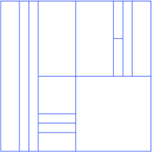
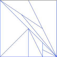
Figure 5: Anisotropic partitions obtained by rectangle split (left) and triangle bisection (right)

The choice between the different splitting scenarios is done by a decision rule which depends on the function $f$. A typical decision rule is to select the split which best decreases the local error. The greedy refinement algorithm therefore reads as follows:

1. Initialization: ${\cal T}_{N_{0}}={\cal D}_{0}$ with $N_{0}:=\#({\cal D}_{0})$.

2. Given ${\cal T}_{N}$ select $T\in{\cal T}_{N}$ that maximizes $e_{m,T}(f)_{T}$.

3. Use the decision rule in order to select the type of split to be performed on $T$.

4. Split $T$ into $K$ elements to obtain ${\cal T}_{N+K-1}$ and return to step 2.

Intuitively, the error equidistribution is ensured by selecting the element that maximizes the local error, while the role of the decision rule is to optimize the shape of the generated elements.

The problem is now to understand if the piecewise polynomial approximations generated by such refinement algorithms satisfy similar convergence properties as those which were established in §4 and §5 when using optimally adapted partitions. We first study the anisotropic refinement algorithm for the simple case of piecewise constant on rectangles, and we give a complete proof of its optimal convergence properties. We then present the anisotropic refinement algorithm for piecewise polynomials on triangulations, and give without proof the available results on its optimal convergence properties.

Remark 6.1

Let us remark that in contrast to the refinement algorithm discussed in §2.3 and 3.3, the partition ${\cal T}_{N}$ may not anymore be identified to a finite subtree within a fixed infinite master tree ${\cal M}$. Instead, for each $f$, the decision rule defines an infinite master tree ${\cal M}(f)$ that depends on $f$. The refinement algorithm corresponds to selecting a finite subtree within ${\cal M}(f)$. Due to the finite number of splitting possibilities for each element, this finite subtree may again be encoded by a number of bits proportional to $N$. Similar to the isotropic refinement algorithm, one may use more sophisticated techniques such as CART in order to select an optimal partition of $N$ elements within ${\cal M}(f)$. On the other hand the selection of the optimal partition within all possible splitting scenarios is generally of high combinatorial complexity.

Remark 6.2

A closely related algorithm was introduced in [26] and studied in [24]. In this algorithm every element is a convex polygon which may be split into two convex polygons by an arbitrary line cut, allowing therefore an infinite number of splitting scenarios. The selected split is again typically the one that decreases most the local error. Although this approach gives access to more possibilities of anisotropic partitions, the analysis of its convergence rate is still an open problem.

6.1 The refinement algorithm for piecewise constants on rectangles

As in §4, we work on the square domain $\Omega=[0,1]^{2}$ and we consider piecewise constant approximation on anisotropic rectangles. At a given stage of the refinement algorithm, the rectangle $T=I\times J$ that maximizes $e_{1,T}(f)_{p}$ is split either vertically or horizontally, which respectively corresponds to split one interval among $I$ and $J$ into two intervals of equal size and leaving the other interval unchanged. As already mentionned in the case of the refinement algorithm discussed in §3.3, we may replace $e_{1,T}(f)_{p}$ by the more computable quantity $\|f-P_{1,T}f\|_{p}$ for selecting the rectangle $T$ of largest local error. Note that the $L^{2}(T)$-projection onto constant functions is simply the average of $f$ on $T$:

$$P_{1,T}f=\frac{1}{|T|}\int_{T}f.$$

If $T$ is the rectangle that is selected for being split, we denote by $(T_{d},T_{u})$ the down and up rectangles which are obtained by a horizontal split of $T$ and by $(T_{l},T_{r})$ the left and right rectangles which are obtained by a vertical split of $T$. The most natural decision rule for selecting the type of split to be performed on $T$ is based on comparing the two quantities

$$e_{T,h}(f)_{p}:=\Bigl{(}e_{1,T_{d}}(f)_{p}^{p}+e_{1,T_{u}}(f)_{p}^{p}\Bigr{)}^{1/p}\;\;{\rm and}\;\;e_{T,v}(f)_{p}:=\Bigl{(}e_{1,T_{l}}(f)_{p}^{p}+e_{1,T_{r}}(f)_{p}^{p}\Bigr{)}^{1/p},$$

which represent the local approximation error after splitting $T$ horizontally or vertically, with the standard modification when $p=\infty$. The decision rule based on the $L^{p}$ error is therefore :

If $e_{T,h}(f)_{p}\leq e_{T,v}(f)_{p}$, then $T$ is split horizontally, otherwise $T$ is split vertically.

As already explained, the role of the decision rule is to optimize the shape of the generated elements. We have seen in §4.1 that in the case where $f$ is an affine function

$$q(x,y)=q_{0}+q_{x}x+q_{y}y,$$

the shape of a rectangle $T=I\times J$ which is optimally adapted to $q$ is given by the relation (4.59). This relation cannot be exactly fullfilled by the rectangles generated by the refinement algorithm since they are by construction dyadic type, and in particular

$$\frac{|I|}{|J|}=2^{j},$$

for some $j\in\rm{{\rm Z}\kern-2.79999pt{\rm Z}}$. We can measure the adaptation of $T$ with respect to $q$ by the quantity

$$a_{q}(T):=\left|\log_{2}\Bigl{(}\frac{|I|\,|q_{x}|}{|J|\,|q_{y}|}\Bigr{)}\right|,$$ (6.91)

which is equal to $0$ for optimally adapted rectangles and is small for “well adapted” rectangles. Inspection of the arguments leading the heuristic error estimate (4.65) in §4.1 or to the more rigourous estimate (4.68) in Theorem 4.2 reveals that these estimates also hold up to a fixed multiplicative constant if we use rectangles which have well adapted shape in the sense that $a_{q_{T}}(T)$ is uniformly bounded where $q_{T}$ is the approximate value of $f$ on $T$.

We notice that for all $q$ such that $q_{x}q_{y}\neq 0$, there exists at least a dyadic rectangle $T$ such that $a_{T}(q)\leq\frac{1}{2}$. We may therefore hope that the refinement algorithm leads to optimal error estimate of a similar form as (4.68), provided that the decision rule tends to generate well adapted rectangles. The following result shows that this is indeed the case when $f$ is exactly an affine function, and when using the decision rule either based on the $L^{2}$ or $L^{\infty}$ error.

Proposition 6.3

Let $q\in\rm\hbox{I\kern-1.99997pt\hbox{P}}_{1}$ be an affine function and let $T$ be a rectangle. If $T$ is split according to the decision rule either based on the $L^{2}$ or $L^{\infty}$ error for this function and if $T^{\prime}$ a child of $T$ obtained from this splitting, one then has

$$a_{q}(T^{\prime})\leq|a_{q}(T)-1|.$$ (6.92)

As a consequence, all rectangles obtained after sufficiently many refinements satisfy $a_{q}(T)\leq 1$.

Proof: We first observe that if $T=I\times J$, the local $L^{\infty}$ error is given by

$$e_{1,T}(q)_{\infty}:=\frac{1}{2}\max\{|q_{x}|\,|I|,|q_{y}|\,|J|\},$$

and the local $L^{2}$ error is given by

$$e_{1,T}(q)_{2}:=\frac{1}{4\sqrt{3}}(q_{x}^{2}|I|^{2}+q_{y}^{2}|J|^{2})^{1/2}.$$

Assume that $T$ is such that $|I|\,|q_{x}|\geq|J|\,|q_{y}|$. In such a case, we find that

$$e_{T,v}(q)_{\infty}=\frac{1}{2}\max\{|q_{x}|\,|I|,|q_{y}|\,|J|/2\}=|q_{x}|\,|I|/2,$$

and

$$e_{T,h}(q)_{\infty}=\frac{1}{2}\max\{|q_{x}|\,|I|/2,|q_{y}|\,|J|\}\leq|q_{x}|\,|I|/2.$$

Therefore $e_{T,h}(q)_{\infty}\leq e_{T,v}(q)_{\infty}$ which shows that the horizontal cut is selected by the decision rule based on the $L^{\infty}$ error. We also find that

$$e_{T,v}(q)_{2}:=\frac{1}{\sqrt{6}}(q_{x}^{2}|I|^{2}+q_{y}^{2}|J|^{2}/4)^{1/2},$$

and

$$e_{T,h}(q)_{2}:=\frac{1}{\sqrt{6}}(q_{x}^{2}|I|^{2}/4+q_{y}^{2}|J|^{2})^{1/2},$$

and therefore $e_{T,h}(q)_{2}\leq e_{T,v}(q)_{2}$ which shows that the horizontal cut is selected by the decision rule based on the $L^{2}$ error. Using the fact that

$$\log_{2}\Bigl{(}\frac{|I|\,|q_{x}|}{|J|\,|q_{y}|}\Bigr{)}\geq 0,$$

we find that if $T^{\prime}$ is any of the two rectangle generated by both decision rules, we have $a_{q}(T^{\prime})=a_{q}(T)-1$ if $a_{q}(T)\geq 1$ and $a_{q}(T^{\prime})=1-a_{q}(T)$ if $a_{q}(T)\leq 1$. In the case where $|I|\,|q_{x}|<|J|\,|q_{y}|$, we reach a similar conclusion observing that the vertical cut is selected by both decision rules. This proves (6.92) $\Box$

Remark 6.4

We expect that the above result also holds for the decision rules based on the $L^{p}$ error for $p\notin\{2,\infty\}$ which therefore also lead to well adapted rectangles when $f$ is an affine. In this sense all decision rules are equivalent, and it is reasonable to use the simplest rules based on the $L^{2}$ or $L^{\infty}$ error in the refinement algorithm that selects the rectangle which maximizes $e_{1,T}(f)_{p}$, even when $p$ differs from $2$ or $\infty$.

6.2 Convergence of the algorithm

From an intuitive point of view, we expect that when we apply the refinement algorithm to an arbitrary function $f\in C^{1}(\Omega)$, the rectangles tend to adopt a locally well adapted shape, provided that the algorithm reaches a stage where $f$ is sufficiently close to an affine function on each rectangle. However this may not necessarily happen due to the fact that we are not ensured that the diameter of all the elements tend to $0$ as $N\to\infty$. Note that this is not ensured either for greedy refinement algorithms based on isotropic elements. However, we have used in the proof of Theorem 3.10 the fact that for $N$ large enough, a fixed portion - say $N/2$ - of the elements have arbitrarily small diameter, which is not anymore guaranteed in the anisotropic setting.

We can actually give a very simple example of a smooth function $f$ for which the approximation produced by the anisotropic greedy refinement algorithm fails to converge towards $f$ due to this problem. Let $\varphi$ be a smooth function of one variable which is compactly supported on $]0,1[$ and positive. We then define $f$ on $[0,1]^{2}$ by

$$f(x,y):=\varphi(4x)-\varphi(4x-1).$$

This function is supported in $[0,1/2]\times[0,1]$. Due to its particular structure, we find that if $T=[0,1]^{2}$, the best approximation in $L^{p}(T)$ is achieved by the constant $c=0$ and one has

$$e_{1,T}(f)_{p}=2^{1/p}\|\varphi\|_{L^{p}}.$$

We also find that $c=0$ is the best approximation on the four subrectangles $T_{d}$, $T_{u}$, $T_{l}$ and $T_{r}$ and that $e_{T,h}(f)_{p}=e_{T_{v}}(f)_{p}=e_{1,T}(f)_{p}$ which means both horizontal and vertical split do not reduce the error. According to the decision rule, the horizontal split is selected. We are then facing a similar situation on $T_{d}$ and $T_{u}$ which are again both split horizontally. Therefore, after $N-1$ greedy refinement steps, the partition ${\cal T}_{N}$ consists of rectangles all of the form $[0,1]\times J$ where $J$ are dyadic intervals, and the best approximation remains $c=0$ on each of these rectangles. This shows that the approximation produced by the algorithm fails to converge towards $f$, and the global error remains

$$e_{1,{\cal T}_{N}}(f)_{p}=2^{1/p}\|\varphi\|_{L^{p}},$$

for all $N>0$.

The above example illustrates the fact that the anisotropic greedy refinement algorithm may be defeated by simple functions that exhibit an oscillatory behaviour. One way to correct this defect is to impose that the refinement of $T=I\times J$ reduces its largest side-length the case where the refinement suggested by the original decision rule does not sufficiently reduce the local error. This means that we modify as follow the decision rule:

Case 1: if $\min\{e_{T,h}(f)_{p},e_{T,v}(f)_{p}\}\leq\rho e_{1,T}(f)_{p}$, then $T$ is split horizontally if $e_{T,h}(f)_{p}\leq e_{T,v}(f)_{p}$ or vertically if $e_{T,h}(f)_{p}>e_{T,v}(f)_{p}$. We call this a greedy split.

Case 2: if $\min\{e_{T,h}(f)_{p},e_{T,v}(f)_{p}\}>\rho e_{1,T}(f)_{p}$, then $T$ is split horizontally if $|I|\leq|J|$ or vertically if $|I|>|J|$. We call this a safety split.

Here $\rho$ is a parameter chosen in $]0,1[$. It should not be chosen too small in order to avoid that all splits are of safety type which would then lead to isotropic partitions. Our next result shows that the approximation produced by the modified algorithm does converge towards $f$.

Theorem 6.5

For any $f\in L^{p}(\Omega)$ or in $C(\Omega)$ in the case $p=\infty$, the partitions ${\cal T}_{N}$ produced by the modified greedy refinement algorithm with parameter $\rho\in]0,1[$ satisfy

$$\lim_{N\to+\infty}e_{1,{\cal T}_{N}}(f)_{p}=0.$$ (6.93)

Proof: Similar to the original refinement procedure, the modified one defines a infinite master tree ${\cal M}:={\cal M}(f)$ with root $\Omega$ which contains all elements that can be generated at some stage of the algorithm applied to $f$. This tree depends on $f$, and the partition ${\cal T}_{N}$ produced by the modified greedy refinement algorithm may be identified to a finite subtree within ${\cal M}(f)$. We denote by ${\cal D}_{j}:={\cal D}_{j}(f)$ the partition consisting of the rectangles of area $2^{-j}$ in ${\cal M}$, which are thus obtained by $j$ refinements of $\Omega$. This partition also depends on $f$.

We first prove that $e_{1,{\cal D}_{j}}(f)_{p}\to 0$ as $j\to\infty$. For this purpose we split ${\cal D}_{j}$ into two sets ${\cal D}_{j}^{g}$ and ${\cal D}_{j}^{s}$. The first set ${\cal D}_{j}^{g}$ consists of the element $T$ for which more than half of the splits that led from $\Omega$ to $T$ were of greedy type. Due to the fact that such splits reduce the local approximation error by a factor $\rho$ and that this error is not increased by a safety split, it is easily cheched by an induction argument that

$$e_{1,{\cal D}_{j}^{g}}(f)_{p}=\Bigl{(}\sum_{T\in{\cal D}_{j}^{g}}e_{1,T}(f)_{p}^{p}\Bigr{)}^{1/p}\leq\rho^{j/2}e_{1,\Omega}(f)_{p}\leq\rho^{j/2}\|f\|_{L^{p}},$$

which goes to $0$ as $j\to+\infty$. This result also holds when $p=\infty$. The second set ${\cal D}_{j}^{s}$ consists of the elements $T$ for which at least half of the splits that led from $\Omega$ to $T$ were safety split. Since two safety splits reduce at least by $2$ the diameter of $T$, we thus have

$$\max_{T\in{\cal D}_{j}^{s}}h_{T}\leq 2^{1-j/4},$$

which goes to $0$ as $j\to+\infty$. From classical properties of density of piecewise constant functions in $L^{p}$ spaces and in the space of continuous functions, it follows that

$$e_{1,{\cal D}_{j}^{s}}(f)_{p}\to 0\;\;{\rm as}\;\;j\to+\infty.$$

This proves that

$$e_{1,{\cal D}_{j}}(f)_{p}=\Bigl{(}e_{1,{\cal D}_{j}^{g}}(f)_{p}^{p}+e_{1,{\cal D}_{j}^{s}}(f)_{p}^{p}\Bigr{)}^{1/p}\to 0\;\;{\rm as}\;\;j\to+\infty,$$

with the standard modification if $p=\infty$.

In order to prove that $e_{1,{\cal T}_{N}}(f)_{p}$ also converges to $0$, we first observe that since $e_{1,{\cal D}_{j}}(f)_{p}\to 0$, it follows that for all $\varepsilon>0$, there exists only a finite number of $T\in{\cal M}(f)$ such that $e_{1,T}(f)_{p}\geq\varepsilon$. In turn, we find that

$$\varepsilon(N):=\max_{T\in{\cal T}_{N}}e_{1,T}(f)_{p}\to 0\;\;{\rm as}\;\;N\to+\infty.$$

For some $j>0$, we split ${\cal T}_{N}$ into two sets ${\cal T}_{N}^{j+}$ and ${\cal T}_{N}^{j-}$ which consist of those $T\in{\cal T}_{N}$ which are in ${\cal D}_{l}$ for $l\geq j$ and $l<j$ respectively. We thus have

$$e_{1,{\cal T}_{N}}(f)_{p}=\Bigl{(}e_{1,{\cal T}_{N}^{j+}}(f)_{p}^{p}+e_{1,{\cal T}_{N}^{j+}}(f)_{p}^{p}\Bigr{)}^{1/p}\\ \leq\Bigl{(}e_{1,{\cal D}_{j}}(f)_{p}^{p}+2^{j}\varepsilon(N)^{p}\Bigr{)}^{1/p}.$$

Since $e_{1,{\cal D}_{j}}(f)_{p}\to 0$ as $j\to+\infty$ and $\varepsilon(N)\to 0$ as $N\to\infty$, and since $j$ is arbitrary, this concludes the proof , with the standard modification if $p=\infty$. $\Box$

6.3 Optimal convergence

We now prove that using the specific value $\rho=\frac{1}{\sqrt{2}}$ the modified greedy refinement algorithm has optimal convergence properties similar to (4.68) in the case where we measure the error in the $L^{\infty}$ norm. Similar results can be obtained when the error is measured in $L^{p}$ with $p<\infty$, at the price of more technicalities.

Theorem 6.6

There exists a constant $C>0$ such that for any $f\in C^{1}(\Omega)$, the partition ${\cal T}_{N}$ produced by the modified greedy refinement algorithm with parameter $\rho=\frac{1}{\sqrt{2}}$ satisfy the asymptotic convergence estimate

$$\limsup_{N\to+\infty}\,N^{1/2}e_{1,{\cal T}_{N}}(f)_{\infty}\leq C\left\|\sqrt{|\partial_{x}f\ \partial_{y}f|}\right\|_{L^{2}}$$ (6.94)

The proof of this theorem requires a preliminary result. Here and after, we use the $\ell^{\infty}$ norm on $\rm\hbox{I\kern-1.99997pt\hbox{R}}^{2}$ for measuring the gradient: for $z=(x,y)\in\Omega$

$$|\nabla f(z)|:=\max\{|\partial_{x}f(z)|,|\partial_{y}f(z)|\},$$

and

$$\|\nabla f\|_{L^{\infty}(T)}:=\sup_{z\in T}|\nabla f(z)|=\max\{\|\partial_{x}f\|_{L^{\infty}(T)},\|\partial_{y}f\|_{L^{\infty}(T)}\}.$$

We recall that the local $L^{\infty}$-error on $T$ is given by

$$e_{1,T}(f)_{\infty}=\frac{1}{2}\left(\max_{z\in T}f(z)-\min_{z\in T}f(z)\right).$$

For the sake of simplicity we define

$$e_{T}(f):=\max_{z\in T}f(z)-\min_{z\in T}f(z)=2e_{1,T}(f)_{\infty},$$

and

$$e_{T,h}f:=2e_{T,h}(f)_{\infty},\quad e_{T,v}(f):=2e_{T,v}(f)_{\infty}.$$

We also recall from the proof of Theorem 6.5 that

$$\varepsilon(N):=\max_{T\in{\cal T}_{N}}e_{T}(f)\to 0\;\;{\rm as}\;\;N\to+\infty.$$

Finally we sometimes use the notation $x(z)$ and $y(z)$ to denote the coordinates of a point $z\in\rm\hbox{I\kern-1.99997pt\hbox{R}}^{2}$.

Lemma 6.7

Let $T_{0}=I_{0}\times J_{0}\in{\cal T}_{M}$ be a dyadic rectangle obtained at some stage $M$ of the refinement algorithm, and let $T=I\times J\in{\cal T}_{N}$ be a dyadic rectangle obtained at some later stage $N>M$ and such that $T\subset T_{0}$. We then have

$$|I|\geq\min\left\{|I_{0}|,\frac{\varepsilon(N)}{4\|\nabla f\|_{L^{\infty}(T_{0})}}\right\}\text{ and }|J|\geq\min\left\{|J_{0}|,\frac{\varepsilon(N)}{4\|\nabla f\|_{L^{\infty}(T_{0})}}\right\}.$$

Proof: Since the coordinates $x$ and $y$ play symmetrical roles, it suffices to prove the first inequality. We reason by contradiction. If the inequality does not hold, there exists a rectangle $T^{\prime}=I^{\prime}\times J^{\prime}$ in the chain that led from $T_{0}$ to $T_{1}$ which is such that

$$|I^{\prime}|<\frac{\varepsilon(N)}{2\|\nabla f\|_{L^{\infty}(T_{0})}},$$

and such that $T^{\prime}$ is split vertically by the algorithm. If this was a safety split, we would have that $|J^{\prime}|\leq|I^{\prime}|$ and therefore

$$e_{T^{\prime}}(f)\leq(|I^{\prime}|+|J^{\prime}|)\|\nabla f\|_{L^{\infty}(T)}\leq 2|I^{\prime}|\|\nabla f\|_{L^{\infty}(T)}<\varepsilon(N),$$

which is a contradiction, since all ancestors of $T$ should satisfy $e_{T^{\prime}}(f)\geq\varepsilon(N)$. Hence this split was necessarily a greedy split.

Let $z_{m}:={\rm Argmin}_{z\in T^{\prime}}f(z)$ and $z_{M}:={\rm Argmax}_{z\in T^{\prime}}f(z)$, and let $T^{\prime\prime}$ be the child of $T^{\prime}$ (after the vertical split) containing $z_{M}$. Then $T^{\prime\prime}$ also contains a point $z^{\prime}_{m}$ such that $|x(z^{\prime}_{m})-x(z_{m})|\leq|I^{\prime}|/2$ and $y(z^{\prime}_{m})=y(z_{m})$. It follows that

$$\begin{array}[]{ll}e_{T^{\prime},v}(f)&=e_{T^{\prime\prime}}(f)\\ &\geq f(z_{M})-f(z^{\prime}_{m})\\ &\geq f(z_{M})-f(z_{m})-\|\partial_{x}f\|_{L^{\infty}(T^{\prime})}|I^{\prime}|/2\\ &\geq e_{T^{\prime}}(f)-\varepsilon(N)/4\\ &\geq\frac{3}{4}e_{T^{\prime}}(f)\\ &>\rho e_{T^{\prime}}(f).\end{array}$$

The error was therefore insufficiently reduced which contradicts a greedy split. $\Box$

Proof of Theorem 6.6: We consider a small but fixed $\delta>0$, we define $h(\delta)$ as the maximal $h>0$ such that

$$\forall z,z^{\prime}\in\Omega,\ |z-z^{\prime}|\leq 2h(\delta)\Rightarrow|\nabla f(z)-\nabla f(z^{\prime})|\leq\delta.$$

For any rectangle $T=I\times J\subset\Omega$, we thus have

$$\begin{array}[]{ll}&e_{T}(f)\geq(\|\partial_{x}f\|_{L^{\infty}(T)}-\delta)\min\{h(\delta),|I|\},\\ &e_{T}(f)\geq(\|\partial_{y}f\|_{L^{\infty}(T)}-\delta)\min\{h(\delta),|J|\}.\end{array}$$ (6.95)

Let $\delta>0$ and $M=M(f,\delta)$ be the smallest value of $N$ such that $\varepsilon(N)<9\delta h(\delta)$. For all $N\geq M$, and therefore $\varepsilon(N)<9\delta h(\delta)$, we consider the partition ${\cal T}_{N}$ which is a refinement of ${\cal T}_{M}$. For any rectangle $T_{0}=I_{0}\times J_{0}\in{\cal T}_{M}$, we denote by ${\cal T}_{N}(T_{0})$ the set of rectangles of ${\cal T}_{N}$ that are contained $T_{0}$. We thus have

$${\cal T}_{N}:=\cup_{T_{0}\in{\cal T}_{M}}{\cal T}_{N}(T_{0}),$$

and ${\cal T}_{N}(T_{0})$ is a partition of $T_{0}$. We shall next bound by below the side length of $T=I\times J$ contained in ${\cal T}_{N}(T_{0})$, distinguishing different cases depending on the behaviour of $f$ on $T_{0}$.

Case 1. If $T_{0}\in{\cal T}_{M}$ is such that $\|\nabla f\|_{L^{\infty}(T_{0})}\leq 10\delta$, then a direct application of Lemma 6.7 shows that for all $T=I\times J\in{\cal T}_{N}(T_{0})$ we have

$$|I|\geq\min\left\{|I_{0}|,\frac{\varepsilon(N)}{40\delta}\right\}\text{ and }|J|\geq\min\left\{|J_{0}|,\frac{\varepsilon(N)}{40\delta}\right\}$$ (6.96)

Case 2. If $T_{0}\in{\cal T}_{M}$ is such that $\|\partial_{x}f\|_{L^{\infty}(T_{0})}\geq 10\delta$ and $\|\partial_{y}f\|_{L^{\infty}(T_{0})}\geq 10\delta$, we then claim that for all $T=I\times J\in{\cal T}_{N}(T_{0})$ we have

$$|I|\geq\min\left\{|I_{0}|,\frac{\varepsilon(N)}{20\|\partial_{x}f\|_{L^{\infty}(T_{0})}}\right\}\text{ and }|J|\geq\min\left\{|J_{0}|,\frac{\varepsilon(N)}{20\|\partial_{x}f\|_{L^{\infty}(T_{0})}}\right\},$$ (6.97)

and that furthermore

$$|T_{0}|\ \|\partial_{x}f\|_{L^{\infty}(T_{0})}\|\partial_{y}f\|_{L^{\infty}(T_{0})}\leq\left(\frac{10}{9}\right)^{2}\int_{R^{*}}|\partial_{x}f\ \partial_{y}f|dxdy.$$ (6.98)

This last statement easily follows by the following observation: combining (6.95) with the fact that $\|\partial_{x}f\|_{L^{\infty}(T_{0})}\geq 10\delta$ and $\|\partial_{y}f\|_{L^{\infty}(T_{0})}\geq 10\delta$ and that $e_{T}(f)\leq\varepsilon(N)\leq 9\delta h(\delta)$, we find that for all $z\in T_{0}$

$$|\partial_{x}f(z)|\geq\|\partial_{x}f\|_{L^{\infty}(T_{0})}-\delta\geq\frac{9}{10}\|\partial_{x}f\|_{L^{\infty}(T_{0})},$$

and

$$|\partial_{y}f(z)|\geq\|\partial_{y}f\|_{L^{\infty}(T_{0})}-\delta\geq\frac{9}{10}\|\partial_{y}f\|_{L^{\infty}(T_{0})},$$

Integrating over $T_{0}$ yields (6.98). Moreover for any rectangle $T\subset T_{0}$, we have

$$\frac{9}{10}\leq\frac{e_{T}(f)}{\|\partial_{x}f\|_{L^{\infty}(T_{0})}|I|+\|\partial_{y}f\|_{L^{\infty}(T_{0})}|J|}\leq 1.$$ (6.99)

Clearly the two inequalities in (6.97) are symmetrical, and it suffices to prove the first one. Similar to the proof of Lemma 6.7, we reason by contradiction, assuming that a rectangle $T^{\prime}=I^{\prime}\times J^{\prime}$ with $|I^{\prime}|\|\partial_{x}f\|_{L^{\infty}(T_{0})}<\frac{\varepsilon(N)}{10}$ was split vertically by the algorithm in the chain leading from $T_{0}$ to $T$. A simple computation using inequality (6.99) shows that

$$\frac{e_{T^{\prime},h}(f)}{e_{T^{\prime}}(f)}\leq\frac{e_{T^{\prime},h}(f)}{e_{T^{\prime},v}(f)}\leq\frac{5}{9}\times\frac{1+2\sigma}{1+\sigma/2}\ \text{ with }\ \sigma:=\frac{\|\partial_{x}f\|_{L^{\infty}(T_{0})}|I^{\prime}|}{\|\partial_{y}f\|_{L^{\infty}(T_{0})}|J^{\prime}|}.$$

In particular if $\sigma<0.2$ the algorithm performs a horizontal greedy split on $T^{\prime}$, which contradicts our assumption. Hence $\sigma\geq 0.2$, but this also leads to a contradiction since

$$\varepsilon(N)\leq e_{T^{\prime}}(f)\leq\|\partial_{x}f\|_{L^{\infty}(T_{0})}|I^{\prime}|+\|\partial_{y}f\|_{L^{\infty}(T_{0})}|J^{\prime}|\leq(1+\sigma^{-1})\frac{\varepsilon(N)}{10}<\varepsilon(N)$$

Case 3. If $T_{0}\in{\cal T}_{M}$ be such that $\|\partial_{x}f\|_{L^{\infty}(T_{0})}\leq 10\delta$ and $\|\partial_{y}f\|_{L^{\infty}(T_{0})}\geq 10\delta$, we then claim that for all $T=I\times J\in{\cal T}_{N}(T_{0})$ we have

$$|I|\geq\min\left\{|I_{0}|,\frac{\varepsilon(N)}{C\delta}\right\}\text{ and }|J|\geq\min\left\{|J_{0}|,\frac{\varepsilon(N)}{4\|\nabla f\|_{L^{\infty}}}\right\},\text{ with }C=200,$$ (6.100)

with symmetrical result if $T_{0}$ is such that $\|\partial_{x}f\|_{L^{\infty}(T_{0})}\geq 10\delta$ and $\|\partial_{y}f\|_{L^{\infty}(T_{0})}\leq 10\delta$. The second part of (6.100) is a direct consequence of Lemma 6.7, hence we focus on the first part. Applyting the second inequality of (6.95) to $T=T_{0}$, we obtain

$$9\delta h(\delta)>e_{T_{0}}(f)\geq(\|\partial_{y}f\|_{L^{\infty}}(T_{0})-\delta)\min\{h(\delta),|J_{0}|\}\geq 9\delta\min\{h(\delta),|J_{0}|\},$$

from which we infer that $|J_{0}|\leq h(\delta)$. If $z_{1},z_{2}\in T_{0}$ and $x(z_{1})=x(z_{2})$ we therefore have $|\partial_{y}f(z_{1})|\geq|\partial_{y}f(z_{2})|-\delta$. It follows that for any rectangle $T=I\times J\subset T_{0}$ we have

$$(\|\partial_{y}f\|_{L^{\infty}(T)}-\delta)|J|\leq e_{T}(f)\leq\|\partial_{y}f\|_{L^{\infty}(T)}|J|+10\delta|I|.$$ (6.101)

We then again reason by contradiction, assuming that a rectangle $T^{\prime}=I^{\prime}\times J^{\prime}$ with $|I^{\prime}|\leq\frac{2\varepsilon(N)}{C\delta}$ was split vertically by the algorithm in the chain leading from $T_{0}$ to $T$. If $\|\partial_{y}f\|_{L^{\infty}(T^{\prime})}\leq 10\delta$, then $\|\nabla f\|_{L^{\infty}(T^{\prime})}\leq 10\delta$ and Lemma 6.7 shows that $T^{\prime}$ should not have been split vertically, which is a contradiction. Otherwise $\|\partial_{y}f\|_{L^{\infty}(T^{\prime})}-\delta\geq\frac{9}{10}\|\partial_{y}f\|_{L^{\infty}(T^{\prime})}$, and we obtain

$$(1-20/C)e_{T^{\prime}}(f)\leq\|\partial_{y}f\|_{L^{\infty}(T^{\prime})}|J^{\prime}|\leq\frac{10}{9}e_{T^{\prime}}(f).$$ (6.102)

We now consider the children $T^{\prime}_{v}$ and $T^{\prime}_{h}$ of $T^{\prime}$ of maximal error after a horizontal and vertical split respectively, and we inject (6.102) in (6.101). It follows that

$$\begin{array}[]{ll}e_{T^{\prime},h}(f)&=e_{T^{\prime}_{h}}(f)\\ &\leq\|\partial_{y}f\|_{L^{\infty}(T^{\prime})}|J^{\prime}|/2+10\delta|I^{\prime}|\\ &\leq\frac{5}{9}e_{T^{\prime}}(f)+20\varepsilon(N)/C\\ &\leq(\frac{5}{9}+20/C)e_{T^{\prime}}(f)=\frac{59}{90}e_{T^{\prime}}(f),\end{array}$$

and

$$\begin{array}[]{ll}e_{T^{\prime},v}(f)&=e_{T^{\prime}_{h}}(f)\\ &\geq(\|\partial_{y}f\|_{L^{\infty}(T^{\prime})}-\delta)|J|\\ &\geq\frac{9}{10}\|\partial_{y}f\|_{L^{\infty}(T^{\prime})}|J^{\prime}|\\ &\geq\frac{9}{10}(1-20/C)e_{T^{\prime}}(f)=\frac{81}{100}e_{T^{\prime}}(f).\end{array}$$

Therefore $e_{T^{\prime},v}(f)>e_{T^{\prime},h}(f)$ which is a contradiction, since our decision rule would then select a horizontal split.

We now choose $N$ large enough so that the minimum in (6.96), (6.97) and (6.100) is are always equal to the second term. For all $T\in{\cal T}_{N}(T_{0})$, we respectively find that

$$\frac{\varepsilon(N)^{2}}{|T|}\leq C\left\{\begin{array}[]{ccl}\delta^{2}&\text{ if }&\|\nabla f\|_{L^{\infty}(T_{0})}\leq 10\delta\\ \frac{1}{|T_{0}|}\int_{T_{0}}|\partial_{x}f\ \partial_{y}f|&\text{ if }&\|\partial_{x}f\|_{L^{\infty}(T_{0})}\geq 10\delta\text{ and }\|\partial_{y}f\|_{L^{\infty}(T_{0})}\geq 10\delta\\ \delta\|\nabla f\|_{L^{\infty}}&\text{ if }&\|\partial_{x}f\|_{L^{\infty}(T_{0})}\leq 10\delta\text{ and }\|\partial_{y}f\|_{L^{\infty}(T_{0})}\geq 10\delta\text{ (or reversed).}\end{array}\right.$$

with $C=\max\{40^{2},\ 20^{2}(10/9)^{2},\ 800\}=1600$. For $z\in\Omega$, we set $\psi(z):=\frac{1}{|T|}$ where $T\in{\cal T}_{N}$ such $z\in T$, and obtain

$$N=\#({\cal T}_{N})=\int_{\Omega}\psi\leq C\varepsilon(N)^{-2}\left(\int_{\Omega}|\partial_{x}f\ \partial_{y}f|dxdy+\delta\|\nabla f\|_{L^{\infty}}+\delta^{2}\right).$$

Taking the limit as $\delta\to 0$, we obtain

$$\limsup_{N\to\infty}\,N^{\frac{1}{2}}\|f-f_{N}\|_{L^{\infty}}\leq 20\left\|\sqrt{|\partial_{x}f\partial_{y}f|}\right\|_{L^{2}},$$

which concludes the proof. $\Box$

Remark 6.8

The proof of the Theorem can be adapted to any choice of parameter $\rho\in]\frac{1}{2},1[$.

6.4 Refinement algorithms for piecewise polynomials on triangles

As in §5, we work on a polygonal domain $\Omega\subset\rm\hbox{I\kern-1.99997pt\hbox{R}}^{2}$ and we consider piecewise polynomial approximation on anisotropic triangles. At a given stage of the refinement algorithm, the triangle $T$ that maximizes $e_{m,T}(f)_{p}$ is split from one of its vertices $a_{i}\subset\{a_{1},a_{2},a_{3}\}$ towards the mid-point $b_{i}$ of the opposite edge $e_{i}$. Here again, we may replace $e_{m,T}(f)_{p}$ by the more computable quantity $\|f-P_{m,T}f\|_{p}$ for selecting the triangle $T$ of largest local error.

If $T$ is the triangle that is selected for being split, we denote by $(T_{i}^{\prime},T_{i}^{\prime\prime})$ the two children which are obtained when $T$ is split from $a_{i}$ towards $b_{i}$. The most natural decision rule is based on comparing the three quantities

$$e_{T,i}(f)_{p}:=\Bigl{(}e_{m,T_{i}^{\prime}}(f)_{p}^{p}+e_{m,T_{i}^{\prime\prime}}(f)_{p}^{p}\Bigr{)}^{1/p},\;\;i=1,2,3.$$

which represent the local approximation error on $T$ after the three splitting options, with the standard modification when $p=\infty$. The decision rule based on the $L^{p}$ error is therefore :

$T$ is split from $a_{i}$ towards $b_{i}$ for an $i$ that minimizes $e_{T,i}(f)_{p}$.

A convergence analysis of this anisotropic greedy algorithm is proposed in [21] in the case of piecewise affine functions corresponding to $m=2$. Since it is by far more involved than the convergence analysis presented in §6.1, §6.2 and §6.3 for piecewise constants on rectangles, but possess several similar features, we discuss without proofs the main available results and we also illustrate their significance through numerical tests.

No convergence analysis is so far available for the case of higher order piecewise polynomial $m>2$, beside a general convergence theorem similar to Theorem 6.5. The algorithm can be generalized to simplices in dimension $d>2$. For instance, a $3$-d simplex can be split into two simplices by a plane connecting one of its edges to the midpoint of the opposite edge, allowing therefore between $6$ possibilities.

As remarked in the end of §6.1, we may use a decision rule based on a local error measured in another norm than the $L^{p}$ norm for which we select the element $T$ of largest local error. In [21], we considered the “$L^{2}$-projection” decision rule based on minimizing the quantity

$$e_{T,i}(f)_{2}:=\Bigl{(}\|f-P_{2,T_{i}^{\prime}}(f)\|_{L^{2}(T_{i}^{\prime})}^{2}+\|f-P_{2,T_{i}^{\prime\prime}}(f)\|_{L^{2}(T_{i}^{\prime\prime})}^{2}\Bigr{)}^{1/2},$$

as well as the “$L^{\infty}$-interpolation” decision rule based on minimizing the quantity

$$d_{T,i}(f)_{2}:=\|f-I_{2,T_{i}^{\prime}}(f)\|_{L^{\infty}(T_{i}^{\prime})}+\|f-I_{2,T_{i}^{\prime\prime}}(f)\|_{L^{\infty}(T_{i}^{\prime\prime})},$$

where $I_{2,T}$ denotes the local interpolation operator: $I_{2,T}(f)$ is the affine function that is equal to $f$ at the vertices of $T$. Using either of these two decision rules, it is possible to prove that the generated triangles tend to adopt a well adapted shape.

In a similar way to the algorithm for piecewise constant approximation on rectangles, we first discuss the behaviour of the algorithm when $f$ is exactly a quadratic function $q$. Denoting by ${\bf q}$ its the homogeneous part of degree $2$, we have seen in §5.1 that when ${\rm det}({\bf q})\neq 0$, the approximation error on an optimally adapted triangle $T$ is given by

$$e_{2,T}(q)_{p}=e_{2,T}(q)_{p}=|T|^{1/\tau}K_{2,p}({\bf q}),\;\;\frac{1}{\tau}:=\frac{1}{p}+1.$$

We can measure the adaptation of $T$ with respect to ${\bf q}$ by the quantity

$$\sigma_{{\bf q}}(T)_{p}=\frac{e_{2,T}({\bf q})_{p}}{|T|^{1/\tau}K_{2,p}({\bf q})},$$

which is equal to $1$ for optimally adapted triangles and small for “well adapted” triangles. It is easy to check that the functions $({\bf q},T)\mapsto\sigma_{T}({\bf q})_{p}$ are equivalent for all $p$, similar to the shape functions $K_{2,p}$ as observed in §5.2.

The following theorem, which is a direct consequence of the results in [21], shows that the decision rule tends to make “most triangles” well adapted to ${\bf q}$.

Theorem 6.9

There exists constants $0<\theta,\mu<1$ and a constant $C_{p}$ that only depends on $p$ such that the following holds. For any ${\bf q}\in\rm\hbox{I\kern-1.99997pt\hbox{H}}_{2}$ such that ${\rm det}({\bf q})\neq 0$ and any triangle $T$, after $j$ refinement levels of $T$ according to the decision rule, a proportion $1-\theta^{j}$ of the $2^{j}$ generated triangles $T^{\prime}$ satisfies

$$\sigma_{{\bf q}}(T^{\prime})_{p}\leq\min\{\mu^{j}\sigma_{{\bf q}}(T)_{p},C_{p}\}.$$ (6.103)

As a consequence, for $j>j({\bf q},T)=-\frac{\log C_{p}-\log(\sigma_{{\bf q}}(T)_{p})}{\log\mu}$ one has

$$\sigma_{{\bf q}}(T^{\prime})_{p}\leq C_{p},$$ (6.104)

for a proportion $1-\theta^{j}$ of the $2^{j}$ generated triangles $T^{\prime}$.

This result should be compared to Proposition 6.3 in the case of rectangles. Here it is not possible to show that all triangles become well adapted to $q$, but a proportion that tends to $1$ does. It is quite remarkable that with only three splitting options, the greedy algorithm manages to drive most of the triangles to a near optimal shape. We illustrate this fact on Figure 6, in the case of the quadratic form ${\bf q}(x,y):=x^{2}+100y^{2}$, and an initial triangle $T$ which is equilateral for the euclidean metric and therefore not well adapted to ${\bf q}$. Triangles such that $\sigma_{{\bf q}}(T^{\prime})_{2}\leq C_{2}$ are displayed in white, others in grey. We observe the growth of the proportion of well adapted triangles as the refinement level increases.

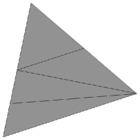
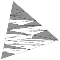
Figure 6: Greedy refinement for ${\bf q}(x,y):=x^{2}+100y^{2}$: $j=2$ (left), $j=5$ (center), $j=8$ (right).

From an intuitive point of view, we expect that when we apply the anisotropic greedy refinement algorithm to an arbitrary function $f\in C^{2}(\Omega)$, the triangles tend to adopt a locally well adapted shape, provided that the algorithm reaches a stage where $f$ is sufficiently close to an quadratic function on each triangle. As in the case of the greedy refinement algorithm for rectangles, this may not always be the case. It is however possible to prove that this property holds in the case of strictly convex or concave functions, using the “$L^{\infty}$-interpolation” decision rule. This allows to prove in such a case that the approximation produced by the anisotropic greedy algorithm satisfies an optimal convergence estimate in accordance with Theorem 5.2. These results from [21] can be summarized as follows.

Theorem 6.10

If $f$ is a $C^{2}$ function such that $d^{2}f(x)\geq\alpha I$ or $d^{2}f(x)\leq-\alpha I$, for all $x\in\Omega$ and some $\alpha>0$, then the triangulation generated by the anisotropic greedy refinement algorithm (with the $L^{\infty}$-interpolation decision rule) satisfies

$$\lim_{N\to+\infty}\max_{T\in{\cal T}_{N}}h_{T}=0.$$ (6.105)

Moreover, there exists a constant $C>0$ such that for any such $f$, the approximation produced by the anisotropic greedy refinement algorithm satisfies the asymptotic convergence estimate

$$\limsup_{N\to+\infty}\,Ne_{2,{\cal T}_{N}}(f)_{p}\leq C\left\|\sqrt{|{\rm det}(d^{2}f)|}\right\|_{L^{\tau}},\;\;\frac{1}{\tau}:=\frac{1}{p}+1.$$ (6.106)

For a non-convex function, we are not ensured that the diameter of the elements tends to $0$ as $N\to\infty$, and similar to the greedy algorithm for rectangles, it is possible to produce examples of smooth functions $f$ for which the approximation produced by the anisotropic greedy refinement algorithm fails to converge towards $f$. A natural way to modify the algorithm in order to circumvent this problem is to impose a type of splitting that tend to diminish the diameter, such as longest edge or newest vertex bisection, in the case where the refinement suggested by the original decision rule does not sufficiently reduce the local error. This means that we modify as follow the decision rule:

Case 1: if $\min\{e_{T,1}(f)_{p},e_{T,2}(f)_{p},e_{T,3}(f)_{p}\}\leq\rho e_{2,T}(f)_{p}$, then split $T$ from $a_{i}$ towards $b_{i}$ for an $i$ that minimizes $e_{T,i}(f)_{p}$. We call this a greedy split.

Case 2: if $\min\{e_{T,1}(f)_{p},e_{T,2}(f)_{p},e_{T,3}(f)_{p}\}>\rho e_{2,T}(f)_{p}$, then split $T$ from the most recently generated vertex or towards its longest edge in the euclidean metric. We call this a safety split.

As in modified greedy algorithm for rectangles, $\rho$ is a parameter chosen in $]0,1[$ that should not be chosen too small in order to avoid that all splits are of safety type which would then lead to isotropic triangulations. It was proved in [20] that the approximation produced by this modified algorithm does converge towards $f$ for any $f\in L^{p}(\Omega)$. The following result also holds for the generalization of this algorithm to higher degree piecewise polynomials.

Theorem 6.11

For any $f\in L^{p}(\Omega)$ or in $C(\Omega)$ in the case $p=\infty$, the approximations produced by the modified anisotropic greedy refinement algorithm with parameter $\rho\in]0,1[$ satisfies

$$\limsup_{N\to+\infty}e_{2,{\cal T}_{N}}(f)_{p}=0.$$ (6.107)

Similar to Theorem 6.6, we may expect that the modified anisotropic greedy refinement algorithm satisfies optimal convergence estimates for all $C^{2}$ function, but this is an open question at the present stage.

Conjecture. There exists a constant $C>0$ and $\rho^{*}\in]0,1[$ such that for any $f\in C^{2}$, the approximation produced by the modified anisotropic greedy refinement algorithm with parameter $\rho\in]\rho^{*},1[$ satisfies the asymptotic convergence estimate (6.106).

We illustrate the performance of the anisotropic greedy refinement algorithm algorithm for a function $f$ which has a sharp transition along a curved edge. Specifically we consider

$$f(x,y)=f_{\delta}(x,y):=g_{\delta}(\sqrt{x^{2}+y^{2}}),$$

where $g_{\delta}$ is defined by $g_{\delta}(r)=\frac{5-r^{2}}{4}$ for $0\leq r\leq 1$, $g_{\delta}(1+\delta+r)=-\frac{5-(1-r)^{2}}{4}$ for $r\geq 0$, $g_{\delta}$ is a polynomial of degree $5$ on $[1,1+\delta]$ which is determined by imposing that $g_{\delta}$ is globally $C^{2}$. The parameter $\delta$ therefore measures the sharpness of the transition. We apply the anisotropic refinement algorithm based on splitting the triangle that maximizes the local $L^{2}$-error and we therefore measure the global error in $L^{2}$.

Figure 7 displays the triangulation ${\cal T}_{10000}$ obtained after $10000$ steps of the algorithm for $\delta=0.2$. In particular, triangles $T$ such that $\sigma_{\bf q}(T)_{2}\leq C_{2}$ - where ${\bf q}$ is the quadratic form associated with $d^{2}f$ measured at the barycenter of $T$ - are displayed in white, others in grey. As expected, most triangles are of the first type therefore well adapted to $f$. We also display on this figure the adaptive isotropic triangulation produced by the greedy tree algorithm based on newest vertex bisection for the same number of triangles.

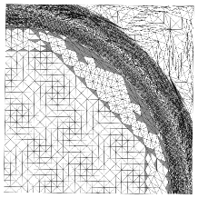
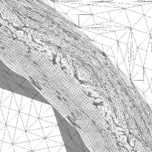
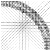
Figure 7: The anisotropic triangulation ${\cal T}_{10000}$ (left), detail (center), isotropic triangulation (right).

Since $f$ is a $C^{2}$ function, approximations by uniform, adaptive isotropic and adaptive anisotropic triangulations all yield the convergence rate $\mathcal{O}(N^{-1})$. However the constant

$$C:=\limsup_{N\to+\infty}Ne_{2,{\cal T}_{N}}(f)_{2},$$

strongly differs depending on the algorithm and on the sharpness of the transition. We denote by $C_{U}$, $C_{I}$ and $C_{A}$ the empirical constants (estimated by $N\|f-f_{N}\|_{2}$ for $N=8192$) in the uniform, adaptive isotropic and adaptive anisotropic case respectively, and by $U(f):=\|d^{2}f\|_{L^{2}}$, $I(f):=\|d^{2}f\|_{L^{2/3}}$ and $A(f):=\|\sqrt{|{\rm det}(d^{2}f)|}\|_{L^{2/3}}$ the theoretical constants suggested by the convergence estimates. We observe on Figure 8. that $C_{U}$ and $C_{I}$ grow in a similar way as $U(f)$ and $I(f)$ as $\delta\to 0$ (a detailed computation shows that $U(f)\approx 10.37\delta^{-3/2}$ and $I(f)\approx 14.01\delta^{-1/2}$). In contrast $C_{A}$ and $A(f)$ remain uniformly bounded, a fact which is in accordance with Theorem 5.4 and reflects the superiority of anisotropic triangulations as the layer becomes thinner and $f_{\delta}$ tends to a cartoon function.

$$\begin{array}[]{c|c|c|c|c|c|c|}\delta&U(f)&I(f)&A(f)&C_{U}&C_{I}&C_{A}\\ \hline\cr 0.2&103&27&6.75&7.87&1.78&0.74\\ 0.1&602&60&8.50&23.7&2.98&0.92\\ 0.05&1705&82&8.48&65.5&4.13&0.92\\ 0.02&3670&105&8.47&200&6.60&0.92\end{array}$$

Figure 8: Comparison between theoretical and empirical convergence constants for uniform, adaptive isotropic and anisotropic refinements, and for different values of $\delta$.

We finally apply the anisotropic refinement algorithm to the numerical image of Figure 4 based on the discretized $L^{2}$ error and using $N=2000$ triangles. We observe on Figure 9 that the ringing artefacts produced by the isotropic greedy refinement algorithm near the edges are strongly reduced. This is due to the fact that the anisotropic greedy refinement algorithm generates long and thin triangles aligned with the edges. We also observe that the quality is slightly improved when using the modified algorithm. Let us mention that a different approach to the approximation of image by adaptive anisotropic triangulations was proposed in [27]. This approach is based on a thinning algorithm, which starts from a fine triangulation and iteratively coarsens it by point removal. The use of adaptive adaptive anisotropic partitions has also strong similarities with thresholding methods based on representations which have more directional selectivity than wavelet decompositions [4, 13, 31, 37]. It is not known so far if these methods satisfy asymptotic error estimates of the same form as (6.106).

         

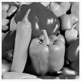
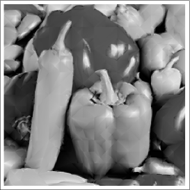
Figure 9: Approximation by $2000$ anisotropic triangles obtained by the greedy (left) and modified (right) algorithm.

References

- [1] F. Alauzet and P.J. Frey, Anisotropic mesh adaptation for CFD computations, Comput. Methods Appl. Mech. Engrg. 194, 5068-5082, 2005.
- [2] B. Alpert, A class of bases in for the sparse representation of integral operators, SIAM J. Math. Anal. 24, 246-262, 1993.
- [3] T. Apel, Anisotropic finite elements: Local estimates and applications, Advances in Numerical Mathematics, Teubner, Stuttgart, 1999.
- [4] F. Arandiga, A. Cohen, R. Donat, N. Dyn and B. Matei, Approximation of piecewise smooth images by edge-adapted techniques, ACHA 24, 225–250, 2008.
- [5] V. Babenko, Y. Babenko, A. Ligun and A. Shumeiko, On Asymptotical Behavior of the Optimal Linear Spline Interpolation Error of Functions, East J. Approx. 12(1), 71–101, 2006.
- [6] Yuliya Babenko, Asymptotically Optimal Triangulations and Exact Asymptotics for the Optimal -Error for Linear Spline Interpolation of Functions, submitted.
- [7] P. Binev and R. DeVore, Fast Computation in Adaptive Tree Approximation, Numerische Mathematik 97, 193-217, 2004.
- [8] P. Binev, W. Dahmen and R. DeVore, Adaptive Finite Element Methods with Convergence Rates, Numerische Mathematik 97, 219–268, 2004.
- [9] J-D. Boissonnat, C. Wormser and M. Yvinec. Locally uniform anisotropic meshing. To appear at the next Symposium on Computational Geometry, june 2008 (SOCG 2008)
- [10] H. Borouchaki, P.J. Frey, P.L. George, P. Laug and E. Saltel, Mesh generation and mesh adaptivity: theory, techniques, in Encyclopedia of computational mechanics, E. Stein, R. de Borst and T.J.R. Hughes ed., John Wiley & Sons Ltd., 2004.
- [11] Sebastien Bougleux and Gabriel Peyré and Laurent D. Cohen. Anisotropic Geodesics for Perceptual Grouping and Domain Meshing. Proc. tenth European Conference on Computer Vision (ECCV’08), Marseille, France, October 12-18, 2008..
- [12] L. Breiman, J.H. Friedman, R.A. Olshen and C.J. Stone, Classification and regression trees, Wadsworth international, Belmont, CA, 1984.
- [13] E. Candes and D. L. Donoho, Curvelets and curvilinear integrals, J. Approx. Theory. 113, 59–90, 2000.
- [14] W. Cao. An interpolation error estimate on anisotropic meshes in and optimal metrics for mesh refinement. SIAM J. Numer. Anal. 45 no. 6, 2368–2391, 2007.
- [15] W. Cao, Anisotropic measure of third order derivatives and the quadratic interpolation error on triangular elements, to appear in SIAM J. Sci. Comput., 2007.
- [16] W. Cao. An interpolation error estimate in based on the anisotropic measures of higher order derivatives. Math. Comp. 77, 265-286, 2008.
- [17] L. Chen, P. Sun and J. Xu, Optimal anisotropic meshes for minimizing interpolation error in -norm, Math. of Comp. 76, 179–204, 2007.
- [18] A. Cohen, Numerical analysis of wavelet methods, Elsevier, 2003.
- [19] A. Cohen, W. Dahmen, I. Daubechies and R. DeVore, Tree-structured approximation and optimal encoding, App. Comp. Harm. Anal. 11, 192–226, 2001.
- [20] A. Cohen, N. Dyn, F. Hecht and J.-M. Mirebeau, Adaptive multiresolution analysis based on anisotropic triangulations, preprint, Laboratoire J.-L.Lions, submitted 2008.
- [21] A. Cohen, J.-M. Mirebeau, Greedy bisection generates optimally adapted triangulations, preprint, Laboratoire J.-L.Lions, submitted 2008.
- [22] A. Cohen, J.-M. Mirebeau, Anisotropic smoothness classes: from finite element approximation to image processing, preprint, Laboratoire J.-L.Lions, submitted 2009.
- [23] W. Dahmen, Adaptive approximation by multivariate smooth splines, J. Approx. Theory 36, 119–140, 1982.
- [24] S. Dahmen, S. Dekel and P. Petrushev, Two-level splits of anisotropic Besov spaces, to appear in Constructive Approximation, 2009.
- [25] S. Dekel, D. Leviatan and M. Sharir, On Bivariate Smoothness Spaces Associated with Nonlinear Approximation, Constructive Approximation 20, 625–646, 2004
- [26] S. Dekel and D. Leviathan, Adaptive multivariate approximation using binary space partitions and geometric wavelets, SIAM Journal on Numerical Analysis 43, 707–732, 2005.
- [27] L. Demaret, N. Dyn, M. Floater and A. Iske, Adaptive thinning for terrain modelling and image compression, in Advances in Multiresolution for Geometric Modelling, N.A. Dodgson, M.S. Floater, and M.A. Sabin (eds.), Springer-Verlag, Heidelberg, 321-340, 2005.
- [28] R. DeVore, Nonlinear approximation, Acta Numerica 51-150, 1998
- [29] R. DeVore and G. Lorentz, Constructive Approximation, Springer, 1993.
- [30] R. DeVore and X.M. Yu, Degree of adaptive approximation, Math. of Comp. 55, 625–635.
- [31] D. Donoho, Wedgelets: nearly minimax estimation of edges, Ann. Statist. 27(3), 859–897, 1999.
- [32] D. Donoho, CART and best basis: a connexion, Ann. Statist. 25(5), 1870–1911, 1997.
- [33] W. Dörfler, A convergent adaptive algorithm for Poisson’s equation, SIAM J. Numer. Anal. 33, 1106–1124, 1996.
- [34] P.J. Frey and P.L. George, Mesh generation. Application to finite elements, Second edition. ISTE, London; John Wiley & Sons, Inc., Hoboken, NJ, 2008.
- [35] J.-P. Kahane, Teoria constructiva de functiones, Course notes, University of Buenos Aires, 1961.
- [36] B. Karaivanov and P. Petrushev, Nonlinear piecewise polynomial approximation beyond Besov spaces, Appl. Comput. Harmon. Anal. 15(3), 177-223, 2003.
- [37] E. Le Pennec and S. Mallat, Bandelet image approximation and compression, SIAM Journal of Multiscale Modeling. and Simulation, 4(3), 992–1039, 2005.
- [38] S. Mallat A Wavelet Tour of Signal Processing - The sparse way, 3rd Revised edition, Academic Press, 2008.
- [39] J.-M. Mirebeau, Optimally adapted finite element meshes, preprint, Laboratoire J.-L.Lions, submitted 2009.
- [40] P. Morin, R. Nochetto and K. Siebert, Convergence of adaptive finite element methods, SIAM Review 44, 631–658, 2002.
- [41] M.C. Rivara, New longest-edge algorithms for the renement and/or improvement of unstructured triangulations, Int. J. Num. Methods 40, 3313–3324, 1997.
- [42] E. M. Stein, Singular integral and differentiability properties of functions, Princeton University Press, 1970.
- [43] R. Stevenson, An optimal adaptive finite element method, SIAM J. Numer. Anal., 42(5), 2188–2217, 2005.
- [44] R. Verfurth, A Review of A Posteriori Error Estimation and Adaptive Mesh-Refinement Techniques, Wiley-Teubner, 1996.
- [45] The 2-d anisotropic mesh generator BAMG: http://www.freefem.org/ff++/ (included in the FreeFem++ software)