The SWELLS survey. II.
Breaking the disk-halo degeneracy in the spiral galaxy gravitational lens SDSS J2141$-$0001 .

Abstract

The degeneracy among the disk, bulge and halo contributions to galaxy rotation curves prevents an understanding of the distribution of baryons and dark matter in disk galaxies. In an attempt to break this degeneracy, we present an analysis of the strong gravitational lens SDSS J2141$-$0001, discovered as part of the SLACS survey. The lens galaxy is a high inclination, disk dominated system. We present new Hubble Space Telescope multicolor imaging, gas and stellar kinematics data derived from long-slit spectroscopy, and K-band laser guide star adaptive optics imaging, both from the Keck telescopes. We model the galaxy as a sum of concentric axisymmetric bulge, disk and halo components and infer the contribution of each component, using information from gravitational lensing and gas kinematics. This analysis yields a best-fitting total (disk plus bulge) stellar mass of $\log_{10}(M_{*}/{\rm M_{\odot}})=10.99^{+0.11}_{-0.25}$. The photometric data combined with stellar population synthesis models yield $\log_{10}(M_{*}/{\rm M_{\odot}})=10.97\pm 0.07$, and $11.21\pm 0.07$ for the Chabrier and Salpeter IMFs, respectively. Assuming no cold gas, a Salpeter IMF is marginally disfavored, with a Bayes factor of 2.7. Accounting for the expected gas fraction of $\simeq 20\%$ reduces the lensing plus kinematics stellar mass by $0.10\pm 0.05$ dex, resulting in a Bayes factor of 11.9 in favor of a Chabrier IMF. The dark matter halo is roughly spherical, with minor to major axis ratio $q_{3,\rm h}=0.91^{+0.15}_{-0.13}$. The dark matter halo has a maximum circular velocity of $V_{\rm max}=276^{+17}_{-18}\,\rm km\,s^{-1}$, and a central density parameter of $\log_{10}\Delta_{V/2}=5.9^{+0.9}_{-0.5}$. This is higher than predicted for uncontracted dark matter haloes in $\Lambda$CDM cosmologies, $\log_{10}\Delta_{V/2}=5.2$, suggesting that either the halo has contracted in response to galaxy formation, or that the halo has a higher than average concentration. Larger samples of spiral galaxy strong gravitational lenses are needed in order to distinguish between these two possibilities. At 2.2 disk scale lengths the dark matter fraction is $f_{\rm DM}=0.55^{+0.20}_{-0.15}$, suggesting that SDSS J2141$-$0001 is sub-maximal.

1 Introduction

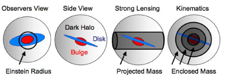
Figure 1: Illustration of the different geometries probed by strong lensing and kinematics. Strong lensing measures mass with a cylinder (or more generally an ellipse), whereas stellar and gas kinematics measure mass within spheres (or more generally ellipsoids).

The discovery of extended flat rotation curves in the outer parts of disk galaxies three decades ago (Bosma 1978; Rubin et al. 1978) was decisive in ushering in the paradigm shift that led to the now standard cosmological model dominated by cold dark matter (CDM). The need for dark matter on cosmological scales is also firmly established from observations of the Cosmic Microwave Background, type Ia Supernovae, weak lensing, and galaxy clustering (see, e.g., Spergel et al. 2007). Numerical simulations of structure formation within the $\Lambda$CDM cosmology make firm predictions for the structure and mass function of dark matter haloes in the absence of baryons (e.g., Navarro, Frenk, & White 1997; Bullock et al. 2001; Macciò et al. 2007; Navarro et al. 2010).

It is still unclear, however, whether this standard model can reproduce the observed properties of the Universe at galactic and sub-galactic scales. There are problems related to the inner density profiles of dark matter haloes (e.g., de Blok et al. 2001; Swaters et al. 2003; Newman et al. 2009), reproducing the zero point of the Tully-Fisher relation (e.g., Mo & Mao 2000; Dutton et al. 2007), and the amount of small-scale substructure (e.g., Klypin et al. 1999; Moore et al. 1999; Stewart et al. 2008). There are three classes of solutions to these problems: those that invoke galaxy formation processes that modify the properties of dark matter haloes; those that change the nature of dark matter itself; and those in which dark matter does not exist. Thus, measuring the density profiles of the dark matter haloes of galaxies of all types is a stringent test for galaxy formation theories.

From an observational point of view, little is known about the detailed distribution of dark matter in the inner regions of disk galaxies, despite the great investment of telescope time and high quality measurements of hundreds of rotation curves (e.g., Carignan & Freeman 1985; Begeman 1987; Courteau 1997; de Blok & McGaugh 1997; Verheijen 1997; Swaters 1999; de Blok et al. 2001; Swaters et al. 2003; Blais-Ouellette et al. 2004; Simon et al. 2005; Noordermeer et al. 2005; Simon et al. 2005; Chemin et al. 2006; Kuzio de Naray 2006; de Blok et al. 2008; Dicaire et al. 2008; Epinat et al. 2008). The fundamental reason is the so-called disk-halo degeneracy: mass models with either maximal or minimal baryonic components fit the rotation curves equally well, leaving the structure of the dark matter halo poorly constrained by the kinematic data alone (e.g., van Albada & Sancisi 1986; van den Bosch & Swaters 2001; Dutton et al. 2005). Stellar population models are able to place constraints on stellar mass-to-light ratios, allowing inference about the baryonic contribution to the overall mass profile. However, there are a number of uncertainties which limit the accuracy of this method (e.g., Conroy et al. 2009, 2010). These include systematic uncertainties such as the unknown stellar initial mass function (IMF), and the treatment of the various stellar evolutionary phases in stellar population synthesis (SPS) models. These result in about a factor of 2 uncertainty in the stellar masses estimated from spectral energy distribution (SED) fitting. Moreover, for a given IMF and SPS model, there are uncertainties in the star formation histories, metallicities and extinction which introduce ($1\sigma$) random errors in measurements of stellar masses for individual galaxies at the level of 0.15 dex (e.g., Bell & de Jong 2001; Auger et al. 2009, Gallazzi & Bell 2009).

Nevertheless, galaxy colours and dynamical mass estimates have been used in combination by various authors to place an upper limit on the stellar mass-to-light ratio normalisation, favoring IMFs more bottom light than Salpeter for spiral galaxies and fast rotating low-mass elliptical galaxies (Bell & de Jong 2001; Cappellari et al. 2006; de Jong & Bell 2007; see, however, Treu et al. 2010, Auger et al. 2010, and van Dokkum & Conroy 2010 for massive ellipticals). However, as theory generally predicts more dark matter in the inner regions of disk galaxies than is consistent with standard IMFs (Dutton et al. 2007; Dutton et al. 2010b) a lower limit to the stellar mass would provide a more useful constraint for $\Lambda$CDM.

Several other methods have been used to try and measure disk galaxy stellar masses, independent of the uncertainties in the IMF. These include: 1) vertical velocity dispersions of low inclination disks (Bottema 1993; Verheijen et al. 2007; Bershady et al. 2010), 2) bars and spiral structure (Weiner et al. 2001; Kranz et al. 2003), and 3) strong gravitational lensing by inclined disks (Maller et al. 2000; Winn et al. 2003). None of these methods have thus far yielded conclusive results.

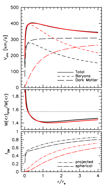
Figure 2: Differences between projected (cylindrical) mass and enclosed (spherical) mass for a bulge-halo system (left) and a disk-halo system (right). For each system two models are shown (in red and black). The models have baryonic mass profiles (short-dashed lines, upper panels) with the same shape but normalizations that differ by a factor of two. The dark matter profiles (long-dashed lines, upper panels) have been chosen so that the total circular velocity curves are close to identical (solid lines, upper panels). For the bulge-halo system the ratio between projected and enclosed masses (middle panels) is independent of the relative contributions of the bulge and halo, which differ significantly between the two models (lower panels). However, for the disk-halo system there is a significant difference between the projected and enclosed masses, especially at radii smaller than the effective radius. This illustrates the potential of strong lensing plus kinematics to break the disk-halo degeneracy.

An approach combining strong gravitational lensing plus kinematics holds great promise, because it takes advantage of the different geometries of disks and haloes, which results in three effects that enable the disk mass to be measured. 1) An inclined disk will present a much higher projected surface density than a face-on disk, with resulting image positions and shapes that depend on the disk mass fraction. 2) An edge-on disk is highly elliptical in projection, more than expected for any realistic dark matter halo, with resulting total mass ellipticity depending on the disk mass fraction 3) Strong lensing measures mass projected along a cylinder (within the Einstein radius), whereas stellar kinematics (rotation and dispersion) measure mass enclosed within spheres (see Figure 1). For spherical mass distributions of stars and dark matter, the ratio between the projected mass within a cylinder of radius, $r$, and the enclosed mass within a sphere of the same radius, $r$, is independent of the relative contribution of the two mass components (left panel Figure 2). Therefore, in order to break the degeneracy one has to assume a radial profile shape for both components (e.g., Treu & Koopmans 2002, 2004; Koopmans & Treu 2003; Koopmans et al. 2006; Treu et al. 2010; Auger et al. 2010). Typically this involves assuming the baryonic mass follows the light, and then assuming a functional form for the dark matter halo. However, for a disk plus halo system, this ratio is dependent on the relative contribution of the two components (right panel Figure 2). Thus if the spherical and cylindrical masses can be measured accurately enough, the disk halo degeneracy can be broken without assuming a specific radial profile shape for either component. Furthermore, strong lensing plus kinematics can place constraints on the 3D shape of the dark matter halo (e.g., Koopmans, de Bruyn, & Jackson 1998; Maller et al. 2000) which is of interest because $\Lambda$CDM haloes are predicted to be non-spherical (e.g. Allgood et al. 2006; Bett et al. 2007; Macciò et al. 2008).

The power of the strong gravitational lensing method has not yet been fully realised, primarily due to the scarcity of known spiral galaxy gravitational lenses. Prior to the SLACS Survey (Bolton et al. 2006, 2008) only a handful of spiral galaxy lenses with suitable inclinations to enable rotation curve measurements were known: Q2237$+$0305 (Huchra et al. 1985; Trott & Webster 2002); B1600$+$434 (Jackson et al. 1995; Jaunsen & Hjorth 1997); PMN J2004$-$1349 (Winn et al. 2003); CXOCY J220132.8$-$320144 (Castander et al. 2006). However, most of these systems are doubly-imaged QSOs which provide minimal constraints on the projected mass density. Q2237$+$0305 is a quadruply-imaged QSO, which gives more robust constraints, but since the Einstein radius is small compared to the size of the galaxy, the lensing is mostly sensitive to the bulge mass, not the halo (Trott et al. 2010; van de Ven et al. 2010).

The final SLACS lens sample (Auger et al. 2009) is comprised of 98 strong galaxy-galaxy lenses, among these, 16 have been classified morphologically as type S or S0. Inspired by this, we have extended the Sloan Digital Sky Survey (hereafter SDSS, York et al. 2000) spectroscopic lens selection technique specifically to spiral galaxy lenses. In the resulting SWELLS survey (Treu et al. , in prep, referred to hereafter as Paper I) we have assembled a larger sample of 20  late-type galaxy-scale gravitational lenses for detailed mass modelling. In this paper, the second of the SWELLS series, we present a detailed and self-consistent mass model of the spiral galaxy lens SDSS J2141$-$0001 (RA=21:41:54.67, DEC=$-$00:01:12.2, J2000), constrained by both kinematic and lensing data. As we will see, this galaxy is disk-dominated, with a disk inclination of $\simeq 80^{\circ}$; this set-up approximately maximises the projected disk mass while allowing an accurate rotation curve to be measured.

The original spectroscopic observations of SDSS J2141$-$0001 were obtained on SDSS plate 989, with fiber 35, on MJD 52468. The latest public SDSS-DR7 (Abazajian et al. 2009) Petrosian magnitudes (uncorrected for extinction) for the lens galaxy are $(u,g,r,i,z)=(20.61,18.62,17.47,16.92,16.48)$ with errors $(0.15,0.01,0.01,0.01,0.02)$. The SDSS measured redshift for the lens galaxy is $z_{\rm d}=0.1380\pm 0.00015$, and the velocity dispersion is $181\pm 14\,\rm km\,s^{-1}$. The spectrum also exhibits nebular emission lines at a background redshift of $z_{\rm s}=0.7127$ (Bolton et al. 2008). With these redshifts the scale in the lens plane is $1\,{\rm arcsec}=2.438\rm\,kpc$, while in the source plane it is $1\,{\rm arcsec}=7.196\rm\,kpc$.

This paper is organised as follows. In Section 2 we present the imaging observations of SDSS J2141$-$0001 from Keck and the Hubble Space Telescope, and then infer the structure of the stellar mass distribution of the galaxy in the presence of its dust from these data in Section 3. With this information in hand we then define a three-component mass model for the galaxy in Section 4, and describe how it is constrained by the imaging data (although we choose not to use the stellar mass inferred from the SED at this stage). In Section 5, we describe the preparation and analysis of the strong lensing data. In Section 6 we present the spectroscopic observations of SDSS J2141$-$0001 from Keck. Then in Section 7 we present fits to the lensing and kinematics data using three combinations: lensing only; kinematics only; and lensing plus kinematics. This joint analysis yields constraints on the stellar mass of the disk and bulge; returning to the stellar masses inferred from the stellar population modelling of the SED we, discuss implications of our results for the stellar IMF in Section 7.2. In Section 7.3 & Section 7.4 we discuss our results for the density and shape of the dark matter halo. We conclude in Section 8.

Throughout, we assume a flat $\Lambda$CDM cosmology with present day matter density, $\Omega_{\rm m}=0.3$, and Hubble parameter, $H_{0}=70\rm\,km\,s^{-1}\,Mpc$. All magnitudes are given in the AB system. Unless otherwise stated, all parameter estimates are the median of the marginalised posterior PDF, and their uncertainties are described by the absolute difference between the median and the 84th and 16th percentiles (such that the error bars enclose 68% of the posterior probability).

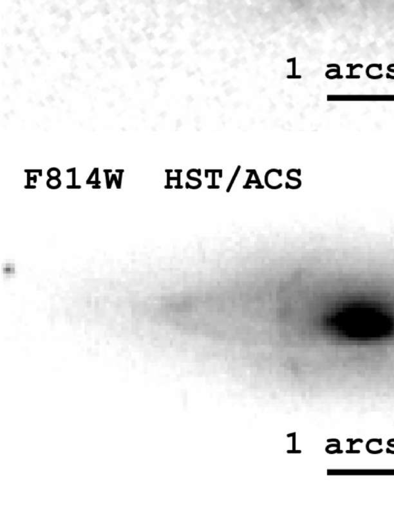
Figure 3: Optical to near-IR high resolution imaging of SDSS J2141$-$0001. Images are 12 arcsec by 6 arcsec, North up, East is left. The lens is a high inclination, disk dominated, and star forming spiral galaxy. The source ($\simeq 1.3$ arcsec to the east of the galaxy center) appears to be multiply imaged in the optical, but is a continuous arc in the near IR.

2 High resolution imaging observations

SDSS J2141$-$0001 has been imaged at $\simeq 0.1$ arcsec FWHM resolution from the optical (with HST) to the NIR (with Keck Laser Guide Star Adaptive Optics). A summary of the imaging observations is given in Table LABEL:tab:imaging, whilst Figure 3 shows the HST and Keck images of SDSS J2141$-$0001. In this section we describe the multi-filter high-resolution imaging data obtained for the SDSS J2141$-$0001 system in some detail.

Table 1: Summary of Imaging Observations

Telescope	Camera	Filter	Integration Time(s)
HST	WFPC2	F450W	4400
HST	WFPC2	F606W	1600
HST	ACS	F814W	420
Keck II	NIRC2-LGS	K’	2700

2.1 ACS/WFPC2 imaging from HST

Hubble Space Telescope (HST) observations of SDSS J2141$-$0001 were obtained on June 12th 2006 with the Advanced Camera for Surveys (ACS), and on April 19th 2009 with the Wide Field Planetary Camera 2 (WFPC2). The ACS observation, in the F814W (420s) filter, was part of the SLACS snapshot programme GO:10587 (PI:Bolton); these data have a pixel scale of $0.05$ arcsec. The WFPC2 observations, in the F450W (4400s) and F606W (1600s) filters, were part of the cycle 16 supplementary programme GO:11978 (PI:Treu). For the WFPC2 observations four sub-exposures were obtained, and the frames drizzled to a pixel scale of $0.05$ arcsec.

The F814W image confirmed the strong lensing nature of this system by showing that the background object was multiply imaged into a three-component arc. It revealed that the lens was a disk dominated galaxy, with a high inclination and dusty disk, and that the bulge was compact and disk like. The F450W and F606W images reveal that the source is blue.

Models for the point spread functions (PSFs) of the ACS and WFPC2 data where obtained by using the program TinyTim (Krist 1995). These PSF models include the effects of sub-pixel dithering and drizzling and have been found to provide adequate models for the true PSF (e.g., Bolton et al. 2008; Auger et al. 2009).

Table 2: Summary of bulge plus disk fits together with stellar masses derived from SED fits with a Chabrier (2003) IMF.

	$q$	$R_{50}[{\rm arcsec}]$	$n$	F450W-K’	F606W-K’	F814W-K’	K’ magnitude	$\log_{10}(M_{*}/M_{\odot})$
Bulge	$0.53\pm 0.02$	$0.26\pm 0.01$	$1.21\pm 0.11$	$3.80\pm 0.04$	$2.40\pm 0.03$	$1.44\pm 0.04$	$17.76\pm 0.28$	$10.26\pm 0.08$
Disk	$0.31\pm 0.02$	$2.53\pm 0.13$	$\equiv 1.0$	$3.04\pm 0.12$	$1.75\pm 0.14$	$1.00\pm 0.12$	$16.25\pm 0.13$	$10.88\pm 0.07$

2.2 NIRC2 imaging from Keck

On August 13th 2009, we imaged SDSS J2141$-$0001 with the Laser Guide Star Adaptive Optics (LGSAO) system on the Keck II telescope. The tip-tilt star had an R-band magnitude of 16.2 and a separation from the science target of $60.4$ arcsec.

The images were taken in the K’-band with the near-infrared camera NIRC2, in wide field format (with a $40\times 40$ arcsec field of view). The pixel scale for this configuration is $0.04\,\rm arcsec\,pix^{-1}$. A total of 45 minutes of exposure was obtained. Individual exposures were 1 minute in duration (divided into two 30-second co-adds). A dither was executed after every set of 5 exposures to improve sky sampling. Dithers were based on a four point box pattern with sides 8 arcsec. The laser was positioned at the center of each frame, rather than fixed on the central galaxy. Observing conditions during the run were good.

The images were processed with the CATS reduction procedure described by Melbourne et al. (2005). A sky frame and a sky flat were created from the individual science exposures after masking out all objects. Frames were then flat-fielded and sky-subtracted. The images were de-warped to correct for known camera distortion. The frames were aligned by centroiding on objects in the field, and finally co-added to produce the final image.

A model for the PSF was derived from observations of a PSF star pair, where the star used for tip-tilt correction is the same distance from the PSF star as the lens galaxy was from its tip tilt star. The star pair observations were made immediately following the lens observations. The PSF star was found to have FHWM=$0.10$ arcsec (2.5 pixels) and a Strehl ratio of 18%.

In the K’-band the extinction of both the lensed images and the lens galaxy light due to dust in the lens galaxy is almost completely absent, revealing a ring like structure, and confirming the disky nature of the bulge. The background object appears to have been lensed into a smooth arc in this filter. The difference between the source structure in the rest-frame NIR and the rest-frame UV/optical is likely due to extinction from the lens galaxy artificially creating the appearance of three distinct images.

3 The stellar mass distribution

We begin our study of the mass distribution of SDSS J2141$-$0001 by inferring the structure of the stellar component from the high resolution imaging data described in the previous section. Following the standard approach (e.g., MacArthur et al. 2003) our strategy is to model the stellar mass distribution as an exponential disk of stars plus a Sérsic profile bulge, with each spatial component consisting of distinct stellar populations. We first fit the surface brightness data to obtain estimates of the shape and profile of the stellar mass density, and then normalise the two profiles by fitting the bulge and disk fluxes in our 4 filters (the spectral energy distribution, or SED) with stellar population synthesis (SPS) models.

3.1 Disk/bulge surface brightness fits

In each band, a 2-dimensional model of the lens galaxy surface brightness was fitted to the high resolution imaging data. The model is composed of two elliptically-symmetric Sérsic profile components, representing the disk and the bulge.

$$\Sigma(x,y)=\Sigma_{0}\exp[-(R/R_{0})^{1/n}]$$ (1)

where $R=\sqrt{x^{2}+y^{2}/q^{2}}$. The Sérsic index $n$ is fixed at 1 for the exponential disk, and left free for the bulge. The remaining parameters for each component are the centroid position $\{x_{c},y_{c}\}$, scale radius $R_{0}$, the axis ratio $q$, and the orientation angle $\phi$. The prior probability distributions were all independent, with uniform priors for $\phi$, $x_{c}$, $y_{c}$ and $q$, and “Jeffreys” ($\propto 1/x$) priors for $R_{0}$ and $n$, between generous upper and lower bounds.

All four bands are fitted simultaneously, with all parameters except for the normalization of the bulge and disk fluxes constrained to be the same in all bands. This approach gives more robust colors of the bulge and disk than is obtained when letting the structural parameters float between bands.

The inferred parameter values for the disk and bulge surface brightness are given in Table LABEL:tab:brewfit. For the bulge component, we find a Sérsic index of $n_{\rm b}=1.21\pm 0.11$, and bulge (luminosity) fraction which increases from $0.11\pm 0.03$ in the F450W filter to $0.20\pm 0.05$ in the K’ band. These values are typical for low-redshift late-type spiral galaxies.

The bulge has a major-axis half-light radius of $R_{\rm 50,b}=0.26\pm 0.01^{\prime\prime}=0.63\pm 0.02\,\rm kpc$, whilst the disk has a major-axis half-light radius of $R_{\rm 50,d}=2.53\pm 0.13^{\prime\prime}=6.17\pm 0.32\,\rm kpc$ corresponding to a disk scale length $R_{\rm d}=1.51^{\prime\prime}\pm 0.08^{\prime\prime}=3.68\pm 0.19\,\rm{\rm kpc}$. The ratio between the bulge half-light radius and the disk scale length is $0.17\pm 0.02$ which is consistent with those found by MacArthur et al. (2003) in a sample of moderately inclined late-type spirals.

The bulge has an observed axis ratio of $q_{\rm b}=0.53\pm 0.02$, while the disk has an observed axis ratio of $q_{\rm d}=0.31\pm 0.02$. For a thin disk the axis ratio equals the cosine of the inclination angle: $q_{\rm d}=\cos(i)$. However, in general disks have a finite thickness, which causes the true inclination to be higher than that inferred from the observed axis ratio. For SDSS J2141$-$0001 we can infer the disk inclination by measuring the axis ratio of the star forming ring, and assuming it is intrinsically circular. This yields an axis ratio $q=0.20\pm 0.02$, and thus $i=78.5\pm 1.2$ degrees.

For an oblate ellipsoid with projected minor-to-major axis ratio, $q$, and inclination, $i$, the 3D minor-to-major axis ratio, $q_{3}$ is given by

$$q_{3}^{2}=(q^{2}-\cos^{2}i)/(1-\cos^{2}i)$$ (2)

Thus for SDSS J2141$-$0001 we infer that the 3D axis ratio of the bulge and disk are $q_{3,\rm b}=0.51\pm 0.02$, and ${q_{3,\rm d}=0.26\pm 0.02}$. The disk thickness that we derive for SDSS J2141$-$0001 is in good agreement with measurements of edge-on spiral galaxies (Kregel et al. 2002). We note that the orientation angles of the disk and bulge components are very close to each other: SDSS J2141$-$0001 appears to be well-modelled by an oblate bulge bisected by a thick, coaxially symmetric disk.

3.2 Stellar population SED fits

The two component model for the surface brightness of SDSS J2141$-$0001 inferred in the previous section can be used to constrain the stellar mass distribution of the galaxy. Given the precision of the shape and profile measurements, the normalisation of the stellar mass distribution is the most uncertain part. Our aim is to constrain this both gravitationally (via dynamical and lensing measurements), and by modelling the stellar populations of the disk and bulge. In this section we describe the latter route.

Assuming each spatial component has a distinct stellar population, we can fit the model photometry for each component to SPS models and infer the stellar mass of each component using the code describe in Auger et al. (2009). We consider stellar populations characterised by either a Chabrier (2003) or Salpeter (1955) IMF and described by 5 parameters: the total stellar mass $M_{*}$, the population age $A$, the exponential star formation burst timescale $\tau$, the metallicity $Z$ and the reddening due to dust, $\tau_{V}$. We employ a uniform prior requiring $9\leq{\rm log_{10}}(M_{*}/{\rm M_{\odot}})\leq 13$, the age is constrained such that star formation began at some (uniformly likely) time between $1\leq z\leq 5$, $\tau$ has an exponential prior with characteristic scale 1 Gyr, and we impose uniform priors on the logarithms of the metallicity and dust extinction such that $-4\leq{\rm log_{10}}Z\leq-1.3$ and $-2\leq{\rm log_{10}}\tau_{V}\leq 0.3$. We note that the priors are the same for the bulge and the disk components but are sufficiently conservative that they do not bias our results. The posterior PDF is sampled as described in Auger et al. (2009).

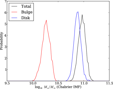
Figure 4: Posterior distributions for the inference on the stellar mass based upon SPS models constrained by the high-resolution photometry, assuming a Chabrier IMF.

Figure 4 shows the marginalised posterior inference on the stellar mass, which we find to be well-constrained for the bulge and disk components. Assuming that both components are well described by a Chabrier IMF, we find $\log_{10}(M_{*,\rm b}/{\rm M_{\odot}})=10.26\pm 0.08$ and $\log_{10}(M_{*,\rm d}/{\rm M_{\odot}})=10.88\pm 0.07$, for the bulge and disk respectively, justifying our description of SDSS J2141$-$0001 as “disk-dominated.” The total stellar mass of SDSS J2141$-$0001 from SED fitting is therefore $\log_{10}(M_{*}/{\rm M_{\odot}})=10.97\pm 0.07$, and the bulge fraction is $f_{\rm bulge}=0.20\pm 0.04$ (the same as in the K’-band light). For a Salpeter IMF the masses are all 0.24 dex higher. We will return to this inference in Section 7.2 below, where we compare it to the stellar mass implied by the gravitational analysis.

Table 3: Summary of mass model priors. Bold indicates an uninformative prior, regular text indicates an informative prior (i.e. that the parameter is virtually fixed). $L\mathcal{N}(a,b^{2})$ denotes a lognormal distribution, with $a$ being the central value for the variable, and $b$ being the standard deviation for the log of the variable. $\mathcal{N}(a,b^{2})$ denotes a normal distribution, with $a$ being the central value and $b$ being the standard deviation. $U(a,b)$ denotes a uniform distribution with lower and upper limits, $a$ and $b$, respectively. For clarity we have arranged the parameters into three groups: free parameters first (with uninformative priors), stellar mass distribution parameters (with priors derived from the SPS modelling of Section 3), and finally nuisance parameters.

parameter	description	prior
$V_{\rm c,h}/\,\rm km\,s^{-1}$	dark halo asymptotic circular velocity	$\mathcal{N}$(280, 502)
$q_{3,\rm h}$	dark halo 3D axis ratio	L$\mathcal{N}$(1, 0.32)
$r_{\rm c,h}$/arcsec	dark halo core radius	U(0.01, 10)
$\log_{10}\left(M_{*}/{\rm M_{\odot}}\right)$	stellar mass	U(10.5,11.4)
$f_{\rm bulge}$	bulge stellar mass fraction	$\mathcal{N}(0.2,0.04^{2})$
$q_{\rm bulge}$	bulge 2D axis ratio	$L\mathcal{N}(0.53,0.03^{2})$
$R_{0,{\rm bulge}}$/arcsec	bulge chameleon size	$L\mathcal{N}(0.094,0.03^{2})$
$\alpha_{\rm bulge}$	bulge chameleon index	0.4892
$q_{\rm disk}$	disk 2D axis ratio	$L\mathcal{N}(0.31,0.03^{2})$
$R_{0,{\rm disk}}$/arcsec	disk chameleon size	$L\mathcal{N}(1.10,0.03^{2})$
$\alpha_{\rm disk}$	disk chameleon index	0.63
$\cos(i)$	cosine of disk inclination angle	0.2
$x_{\rm c}$/arcsec	spatial offset in x direction	$\mathcal{N}(0,0.01^{2})$
$y_{\rm c}/$arcsec	spatial offset in y direction	$\mathcal{N}(0,0.03^{2})$
$\theta$/deg	mass-light position angle offset	$\mathcal{N}(1.7,2.9^{2})$
$\gamma$	lens external shear	$\mathcal{N}(0,0.1^{2})$
$\theta_{\gamma}$/deg	position angle of external shear	$U(0,180)$

4 A three-component galaxy mass model

As indicated in the previous section, it makes sense to consider a stellar mass distribution for SDSS J2141$-$0001 whose profile and spatial shape is tightly constrained by the structural analysis of the surface brightness observed. However, we would like to remain agnostic about the stellar IMF, and instead investigate the stellar mass of the galaxy independently, using strong lensing and stellar kinematics. Since these are sensitive to the total mass of the galaxy, we include a dark matter halo component to the model as well. In this section we describe this 3-component mass model in some detail, including the predictions it makes for the observable effects, and the prior PDFs we assign on the model parameters.

4.1 Description

Based on the results of the previous section, we model the stellar mass distribution of SDSS J2141$-$0001 as a thin, circular exponential disk of stars of mass $M_{*,\rm d}$, co-axial with an oblate bulge of stars of mass $M_{*,\rm b}$. We then assume the galaxy to reside in a dark matter halo that is also axisymmetric, and aligned and concentric with the disk and bulge. This assumption that the galaxy and inner dark matter haloes are aligned is supported by cosmological simulations of disk galaxy formation (e.g., Deason et al. 2011). We note that for our strong lensing analysis it is feasible to allow the position angles of the baryons and dark matter to be offset. However, this would make the model non-axisymmetric and thus make the kinematics considerably harder to model. The surface brightness in our four filters constrains the spatial distribution of stellar mass tightly, under the assumption that the stellar mass-to-light ratios are radially constant; we leave the overall normalisation of the stellar mass distribution as a free parameter.

We do not explicitly include a cold gas disk for two reasons. Firstly, we do not have direct observations of the atomic and molecular gas in SDSS J2141$-$0001. Secondly, observations suggest that the gas fractions for low-redshift luminous spiral galaxies are of order $20\%$ (e.g., Dutton & van den Bosch 2009), and thus do not contribute significantly to the baryonic mass. However, if we were to assume that any cold gas present has the same spatial distribution as the stars, the unknown gas mass could be absorbed into a baryonic mass-to-light ratio that includes the stellar mass-to-light ratio. For the majority of this paper we neglect the cold gas mass, but return to it in the discussion of the IMF (Section 7.2) below.

The three mass components are described as follows:

• Exponential Stellar Disk

• Sérsic Stellar Bulge

• Non-singular Isothermal Ellipsoid (NIE) Dark Matter Halo

This model has 17 parameters in total; they, and their prior PDFs, are given in Table 3. We assign informative priors to all but 4 of these parameters, propagating the uncertainties in the surface brightness fits through to the mass model.

First, we assume the bulge, disk, and halo inclination are all the same, and given by the thin disk axis ratio (0.2), as in Section 3 – we assume that this is known with no uncertainty. As we describe below, we use an approximation to the Exponential profile that allows us to compute predicted observable quantities efficiently – the size parameters of the bulge and disk in that approximation are determined from the results of the previous section, as is (more straightforwardly) the bulge axis ratio. We use the derived value of 1.21 (see Table LABEL:tab:brewfit) for the Bulge Sérsic index, with no uncertainty.

We assume that the disk and bulge are different stellar populations, and so use the independent stellar mass results from the previous section to constrain the bulge mass fraction, $f_{\rm bulge}=M_{*,\rm b}/M_{*}$. As already mentioned, we leave the total stellar mass $M_{*}$ as a free parameter with uniform prior on its logarithm. This is effectively equivalent to assuming that the two components have very similar, although unknown, IMF normalization, We do inform the bounds of this uniform prior using the SPS modelling results, in the following way. Estimating that the lightest conceivable IMF would give stellar masses systematically a factor of two lower than Chabrier, we take the 3-sigma point of the Chabrier PDF in Figure 4 and subtract 0.3 dex to set a lower limit on $\log_{10}\left(M_{*}/{\rm M_{\odot}}\right)$ of 10.5. Likewise, at the high end we take Salpeter to be the heaviest IMF and use the 3-sigma point of the Salpeter PDF in Figure 4 (11.4) as our upper limit on $\log_{10}\left(M_{*}/{\rm M_{\odot}}\right)$. We note that none of our results change if we adopt a higher upper limit to the stellar mass.

This leaves 3 parameters that describe the model dark matter halo: $V_{\rm c,h}$, $r_{\rm c,h}$, and $q_{3,\rm h}$. We allow the axis ratio of the halo to be greater than unity, corresponding to a prolate halo, but use a broad lognormal distribution centred on spherical to encode approximately our expectations. For the halo density profile, the NIE profile has considerable freedom and can represent a much broader range of behaviours than those seen in simulation. Therefore, we adopt physically motivated priors to select the cosmologically motivated subset of parameters combination. Studies of large sets of spiral galaxies, using satellite kinematics and weak galaxy-galaxy lensing, in the context of numerical simulations have shown that the maximum observed circular velocity is typically comparable to the maximum circular velocity of the halo, even though these two maximums occur at vastly different radii (Dutton et al. 2010a). We also know that rotation curves do not keep rising indefinitely, but typically flatten out within a few scale radii of the disk. To inject this information we require that the asymptotic circular velocity of the halo be comparable to that measured via spectroscopy (see § 6 below): in practice we assign a broad Gaussian prior centred on 280 $\,\rm km\,s^{-1}$ with width 50 $\,\rm km\,s^{-1}$ . The prior is chosen to be broad enough – the 3-sigma range of this Gaussian spans the range 130 to 430 $\,\rm km\,s^{-1}$ – not to drive the final inference and yet tight enough to rule out models where the maximum velocity is reached too far out. In addition we impose a uniform prior PDF for the core radius, allowing it to be at most 24 kpc (10”).

In later sections we will introduce the kinematic and lensing data, and then use them to constrain the parameters of this 3-component mass model. However, before getting to the data, in the rest of this section we give the functional forms for each mass component, and the predicted observables resulting from them.

4.2 Three-dimensional component density profiles

The axisymmetric ellipsoidal halo is assumed to have a non-singular isothermal (NIE) profile, which we parametrise in a cylindrical coordinate system in the plane of the galaxy following Keeton & Kochanek (1998):

$$\rho_{\rm NIE}(R,z;V_{\rm c},r_{\rm c},q_{3})=\frac{V_{\rm c}^{2}}{4\pi Gq_{3}}\frac{e}{\sin^{-1}e}\frac{1}{r_{\rm c}^{2}+R^{2}+z^{2}/q_{3}^{2}}.$$ (3)

Here, $V_{\rm c}$ is the asymptotic circular velocity, $r_{\rm c}$ is the core radius, $q_{3}$ is the three dimensional axis ratio, and $e=(1-q_{3}^{2})^{1/2}$ is the eccentricity. For a zero thickness mass distribution ($q_{3}=0$), $e/\sin^{-1}e=2/\pi$. For a spherical mass distribution ($q_{3}=1$), $e/\sin^{-1}e=1$. For a prolate mass distribution ($q_{3}>1$), while $e$ is imaginary, $e/\sin^{-1}e$ is real and greater than 1.

This mass profile is often used in gravitational lens analysis, since its projected mass distribution and deflection angles can be computed analytically (Keeton & Kochanek 1998). This model has been used very successfully to model the total (dark plus stellar) mass profiles of elliptical galaxy lenses (e.g., Bolton et al. 2008). In this work we use the NIE model for the halo alone. While the NIE profile has a constant central density, it is flexible enough to broadly capture the change in the density profile in the central regions that we expect from numerical simulations of dark matter halos (e.g., Navarro et al. 1997).

We would like to model the stellar disk and stellar bulge mass components such that in projection they appear to have exponential and Sérsic profiles respectively. However, we also need 3D distributions for which we can compute predicted rotation curves, as well as projected distributions convenient for lensing calculations. To achieve this we note that the NIE profile can be used to create an approximation to an exponential profile in projection (Maller et al. 2000). This is done by taking the difference of two NIEs. If $\rho_{\rm NIE}(R,z;V_{\rm c},r_{\rm c},q_{3})$ is a softened isothermal ellipsoid, then

$$\rho_{\rm Chm}(R,z;V_{\rm c},r_{\rm c},q_{3},\alpha) = \rho_{\rm NIE}(R,z;V_{\rm c},r_{\rm c},q_{3})$$

$$- \rho_{\rm NIE}(R,z;V_{\rm c},r_{\rm c}/\alpha,q_{3})$$

is a “Chameleon” profile with positive density everywhere, and a finite total mass. In Appendix A we derive new formulae that provide Chameleon approximations to Sérsic profiles of any index (for $1\mathrel{\hbox to0.0pt{\lower 3.0pt\hbox{$\sim$}\hss}\raise 2.0pt\hbox{$<$}}n\mathrel{\hbox to0.0pt{\lower 3.0pt\hbox{$\sim$}\hss}\raise 2.0pt\hbox{$<$}}4$), providing the Chameleon size $r_{\rm c}$ and index $\alpha$ given a Sérsic half light radius $R_{\rm 50}$ and index $n$.

4.3 Predicted rotation curves

For our ellipsoidal mass profiles, we can calculate the rotation velocity, as a function of radius, of a massless test particle moving on a circular orbit in the plane of the galaxy. We refer to this velocity as the circular velocity to distinguish it from the rotation velocity of the stars and gas, which may be lower than the circular velocity due to a velocity dispersion component. The circular velocity profile for the NIE model is (Keeton & Kochanek 1998)

$$\frac{V_{\rm NIE}^{2}(R;V_{\rm c},r_{\rm c},q_{3})}{V_{\rm c}^{2}}=1-\frac{e}{\sin^{-1}e}\frac{r_{\rm c}}{(R^{2}+e^{2}r_{\rm c}^{2})^{1/2}}$$

$$\times\tan^{-1}\left[\frac{(R^{2}+e^{2}r_{\rm c}^{2})^{1/2}}{q_{3}r_{\rm c}}\right],$$ (5)

where again $e=(1-q_{3}^{2})^{1/2}$ is the eccentricity of the mass distribution and the model is normalised so that, asymptotically for $R\rightarrow\infty$, $V_{\rm NIE}(R)\rightarrow V_{c}$. For the special case of a zero thickness mass distribution ($q_{3}=0,e=1$) Equation 4.3 reduces to

$$\frac{V_{\rm NIE}^{2}(R)}{V_{\rm c}^{2}}=1-\frac{r_{\rm c}}{(R^{2}+r_{\rm c}^{2})^{1/2}}.$$ (6)

For the case of a prolate mass distribution ($q_{3}>1$), $e/\sin^{-1}e$ is real, but since $e^{2}<0$, for $(R^{2}+e^{2}r_{\rm c}^{2})<0$ the circular velocity is given by

$$\frac{V_{\rm NIE}^{2}(R)}{V_{\rm c}^{2}}=1-\frac{\tilde{e}}{\sinh^{-1}\tilde{e}}\frac{r_{\rm c}}{(-R^{2}-e^{2}r_{\rm c}^{2})^{1/2}}$$

$$\times\tanh^{-1}\left[\frac{(-R^{2}-e^{2}r_{\rm c}^{2})^{1/2}}{q_{3}r_{\rm c}}\right],$$ (7)

where $\tilde{e}=\sqrt{|e^{2}|}$.

For the chameleon profile the circular velocity is given by the quadratic difference between the circular velocities of the sub-component NIE’s:

$$V^{2}_{\rm chm}(R;V_{\rm c},r_{\rm c},q_{3},\alpha)=V^{2}_{\rm NIE}(R;V_{\rm c},r_{\rm c},q_{3})$$ (8)

$$-V^{2}_{\rm NIE}(R;V_{\rm c},r_{\rm c}/\alpha,q_{3}).$$

Likewise, for the mass model the total circular velocity is given by the quadratic sum of the circular velocities of the bulge, disk, and halo components:

$$V^{2}(R)=V^{2}_{\rm bulge}(R)+V^{2}_{\rm disk}(R)+V^{2}_{\rm halo}(R)$$ (9)

.

4.4 Predicted lensed images

Projecting the three components onto the sky allows us to compute deflection angles and predict the observed gravitational arc, pixel by pixel.

In projection the mass distribution (an oblate or prolate ellipsoid with minor to major axis ratio $q_{3}$) has projected axis ratio $q$ given by

$$q=(q_{3}^{2}\sin^{2}i+\cos^{2}i)^{1/2},$$ (10)

where $i$ is the inclination angle (such that $i=0^{\circ}$ corresponds to a face-on disk, and $i=90^{\circ}$ to an edge-on one). In general the projected axis ratio, $q$, will be closer to unity than the 3D axis ratio, $q_{3}$.

The projected mass density of an NIE model is given by (Keeton & Kochanek 1998):

$$\Sigma_{\rm NIE}(x,y;b,r_{\rm c},q) = \frac{V_{\rm c}^{2}}{4GD_{\rm d}}\frac{e}{\sin^{-1}e}\frac{1}{q\sqrt{r_{c}^{2}+x^{2}+(y/q)^{2}}},$$ (11)

$$= \frac{\Sigma_{\rm crit}b}{2}\frac{1}{q\sqrt{r_{c}^{2}+x^{2}+(y/q)^{2}}}.$$

Here, $D_{\rm d}$ is the angular diameter distance to the lens, and $e$ is again the ellipticity, while in the second line $b$ is the minor axis of the critical curve (and thus $b/q$ is the major axis of the critical curve), and $\Sigma_{\rm crit}$ is the critical surface density of strong lensing:

$$\Sigma_{\rm crit}=\frac{c^{2}}{4\pi G}\frac{D_{\rm s}}{D_{\rm ds}D_{\rm d}},$$ (12)

where $D_{\rm s}$ is the angular diameter distance from the observer to the source, and $D_{\rm ds}$ is the angular diameter distance from the lens to the source. For our assumed cosmology, for SDSS J2141$-$0001 these distances are: $D_{\rm d}=497.6\rm Mpc$, $D_{\rm s}=1510.2\rm Mpc$, $D_{\rm ds}=1179.6\rm Mpc$, and thus the critical density is $\Sigma_{\rm crit}=4285.3\rm M_{\odot}pc^{-2}$.

To explain the parts of Equation 11 a little further, the parameter, $b$, is related to the spherical Einstein radius, $b_{\rm SIS}$, via:

$$b=b_{\rm SIS}(e/\sin^{-1}e),$$ (13)

and the spherical Einstein radius (in radians) is in turn related to the asymptotic circular velocity, $V_{\rm c}$, via:

$$b_{\rm SIS}=2\pi(V_{\rm c}/c)^{2}D_{\rm ds}/D_{\rm s}.$$ (14)

The deflection angles are given by (Keeton & Kochanek 1998)

$$\alpha_{x} = \frac{b}{(1-q^{2})^{1/2}}\tan^{-1}\left[\frac{(1-q^{2})^{1/2}x}{\Psi+r_{\rm c}}\right],$$ (15)

$$\alpha_{y} = \frac{b}{(1-q^{2})^{1/2}}\tanh^{-1}\left[\frac{(1-q^{2})^{1/2}y}{\Psi+q^{2}r_{\rm c}}\right],$$ (16)

where $\Psi^{2}=q^{2}(r_{\rm c}^{2}+x^{2})+y^{2}$. The deflection angles from the three components of the mass distribution can be simply summed, as they are just the first derivatives of the projected (lens) potential of each component, and the potentials of the three components can be summed themselves to give the total potential. Likewise, the Chameleon profile in projection is just the difference between two projected NIE models, and its deflection angles are just the difference between those of its NIE components.

To predict the positions and structure of the lensed images given a set of mass model parameters, we map each observed pixel location back to the source plane using the overall deflection angle map, and look up the surface brightness of a model source at that position. In practice we use a single, elliptically symmetric source with a Sérsic brightness profile, as in e.g., Marshall et al. (2007).

5 Strong Gravitational Lensing Data

We now present the strong gravitational lensing data that we will use to constrain our mass model. We first describe the preparation of the arc imaging data, and then show with a simple lens model the information it contains.

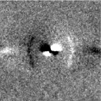
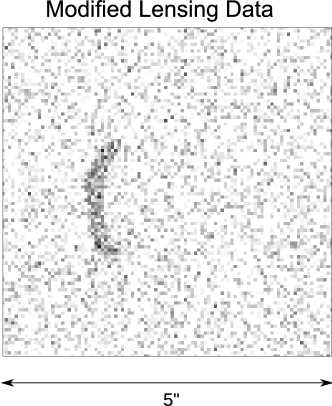
Figure 5: Upper panel: Galaxy subtracted image in the K’-band obtained using a reflection of the image. The lens galaxy is well subtracted near the arc, but there are significant residuals near the center. Lower panel: An arc in the right place, obtained by masking out non-arc features from the image in the upper panel. This was used for the actual fitting, to weaken the fit criterion. Essentially, we want to produce models whose posterior distribution predicts an arc with this morphology, but does not necessarily need to match every pixel.

5.1 The lensed arc likelihood

Due to the strong effects of dust in the lens system, we focus our lensing analysis primarily on the K’-band NIRC2 image. In the K’-band the lens galaxy appears to be much smoother than in the optical, but the light distribution is not able to be modelled by a simple surface brightness profile. This makes subtracting the lens galaxy light difficult. Our goal is to obtain robust parameter inferences with meaningful uncertainties, and so we opt for quite a conservative application of the imaging data. To account for lens subtraction errors, we create an arc image and a goodness of fit statistic that rewards a model for having an arc in the right place, with the right shape, and that is all: we do not require the detailed features of the modified surface brightness profile to be matched.

To achieve this, we first subtracted the galaxy light around the arc by reflecting the galaxy along the minor axis. This method provides a better subtraction than multiple Sérsic components, or a radial bspline model (as used by e.g., Bolton et al. 2006). We then cut out the arc and set the remaining pixels to zero, before adding noise at the level of $\sigma_{15}=15$% of the peak arc brightness. This 15% value is an initial estimate of the appropriate noise level needed to suppress models that predict significant lensed features elsewhere, although faint counter-images are still allowed. The resulting modified image is shown in Figure 5 (lower panel); we also show the lens subtracted image (upper panel), with its uncertain central region. It is not clear whether or not there is a counter-image in the centre of the system. We note that if there is no counter image, then SDSS J2141$-$0001 would be a rare example of galaxy-scale naked cusp lens.

The likelihood function for the modified image data was that used by Brewer & Lewis (2006), Marshall et al. (2007), and others. We assume Gaussian errors of $\sigma_{15}$ on the pixel values ${\mathbf{d}}$; we can predict these pixel values from a model source with parameters $\boldsymbol{\theta}_{\rm s}$ (as described in Section 4.4 above) given lens model parameters $\boldsymbol{\theta}_{\rm m}$. Denoting the predicted data as ${\mathbf{d}^{\rm p}}$, we write down the usual chi-squared misfit function

$$\chi^{2}=\sum_{i}^{\rm pixels}\frac{\left[d_{i}-d^{\rm p}_{i}(\boldsymbol{\theta}_{\rm m},\boldsymbol{\theta}_{\rm s})\right]^{2}}{2\sigma_{15}^{2}}.$$ (18)

We allow the data to inform our understanding of the model uncertainty, by re-scaling the denominator by a factor $T$. This corresponds to increasing or decreasing the perceived errors on the pixel values, and provides a mechanism for avoiding over-fitting the arc structure or allowing models that predict undetected flux. (The symbol $T$ stands for “temperature” – increasing the temperature increases the diffusion of the model around its parameter space.) The likelihood function is then:

$${\rm Pr}({\mathbf{d}}|\boldsymbol{\theta}_{\rm m},\boldsymbol{\theta}_{\rm s})\propto\exp\left(-\frac{1}{2T}\chi^{2}\right)$$ (19)

The value of $T$ selected was 7.5. This was the highest value where the posterior distribution only contained images that resemble the arc morphology. Higher temperatures caused the posterior models to predict substantial flux that is not observed, lower temperatures enforced the fit to the modified image to be too strict. The reason for the two-step procedure (adding noise and then selecting a temperature) is that Nested Sampling provides the results for all temperatures in a single run, whereas tuning the noise level itself would have required large numbers of trial runs.

Using this modified image, and the temperature-raising scheme, allows us to explore an approximate posterior distribution for the lens model parameters that conditions on the presence of an arc with the observed morphology, and nothing else.

Figure 6: Marginalised posterior PDF for the 2D axis ratio, $q$, and circular velocity, $V_{\rm c}$, for a single SIE component model fitted to the strong lensing data. The dashed lines show the median values of $q$ and $V_{\rm c}$.

5.2 Constraints on projected ellipticity and mass

To illustrate the unique information that strong gravitational lensing provides, we first perform a fit to the lensing data with a single singular isothermal ellipsoid (SIE) mass model. The purpose of this exercise is to show that strong lensing places constraints on the axis ratio of the projected mass, as well as the projected mass within the Einstein radius.

Fixing its centroid and orientation to that of the lens surface brightness, our example SIE lens model has two parameters, minor axis Einstein radius $b$, and axis ratio $q$. We assign uniform priors over wide ranges for these parameters, and then explore the posterior PDF using our sampling code (which we introduce in more detail in Section 7 below). We find the circularised Einstein radius to be $\theta_{\rm Ein}=b/\sqrt{q}=0.89^{+0.05}_{-0.08}$ arcsec, and the axis ratio to be $q=0.42^{+0.17}_{-0.12}$. We can transform samples in $b$ and $q$ into the circular velocity, which we expect to be well constrained. Figure 6 shows the marginalised posterior PDF for $q$ and $V_{\rm c}$ – the circular velocity is indeed well-constrained: $V_{\rm c}=254^{+15}_{-18}\,\rm km\,s^{-1}$. The shape of the arc also constrains the ellipticity of the total mass distribution: since in our three-component model the ellipticity of the disk and bulge are fixed, we expect strong lensing to then provide information about the shape of the dark halo.

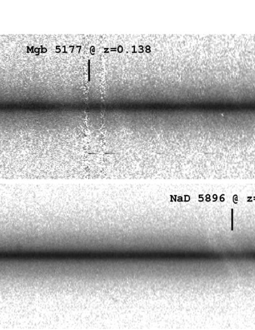
Figure 7: Cutout images of the DEIMOS optical long slit spectrum of SDSS J2141$-$0001 centered on prominent emission and absorption features: Mgb 5177, FeII 5270 from the lens (upper left); NaD 5896 from the lens (lower left); OII 3727 from the source (upper right); and H$\alpha$ 6563, [NII] 6550 6585 from the lens (lower right). The vertical scale is 20 arcsec; the vertical bar is 3 arcsec. Up corresponds to East (left in the images in Figure 3). The ring in the imaging (Fig. 3) corresponds to strong H$\alpha$ emission due to star formation.

6 Gas and Stellar Kinematics Data

The second set of data that we will use to constrain our mass model is a galaxy rotation curve, derived from optical emission and absorption line spectroscopy. In this section we describe the observations, and the rotation curve extraction process, discuss the observed velocity dispersion and our interpretation of it, and then derive the likelihood function that we will use when fitting our mass model.

6.1 Spectroscopic observations with Keck

Major axis ($\rm PA=87^{\circ}$) long-slit spectra were obtained with the DEep Imaging Multi-Object Spectrograph (DEIMOS), and Low Resolution Imaging Spectrograph (LRIS) on the Keck 10-m telescopes.

On October 1st 2008 SDSS J2141$-$0001 was observed with DEIMOS on Keck II. We used the 1200 line grating (corresponding to a pixel scale of $0.32A$) with a 1” width slit resulting in a spectral resolution of $\simeq 1.9A$. The central wavelength was $6500A$, resulting in a wavelength range of $5200-7800A$. We took three exposures of 1200s in seeing conditions of $0.60^{\prime\prime}$. The slit was aligned with the major axis of the galaxy, with $\rm PA=87$. The spectra were reduced using routines developed by D. Kelson (Kelson 2003).

On November 27th 2008 we observed SDSS J2141$-$0001 with LRIS on Keck I. However, the seeing for this observation was considerably worse ($\simeq 1.5^{\prime\prime}$) than that of our DEIMOS observation. This resulted in increased beam-smearing and reduced sensitivity, and thus we focus our kinematic analysis on the DEIMOS observations.

6.2 The observed rotation curve

Cutouts of the DEIMOS long-slit spectrum centered around prominent emission and absorption lines are shown in Figure 7. These show clear signs of rotation in both emission and absorption lines. For the emission lines we measured rotation curves by locally fitting Gaussian line profiles to one-dimensional spectra extracted along the slit. For the absorption lines we measured the rotation and dispersion profile by applying python routines developed by M.W.Auger to one-dimensional spectra extracted along the slit. The upper right panel also shows the spatially offset [O ii] emission lines from the source galaxy.

The extracted rotation curve is shown in the upper panels of Figure 8. The spatial sampling is $\simeq 0.59"$ (5 DEIMOS pixels), corresponding to 1 data point per seeing FWHM. There is good agreement in the rotation curves measured in H$\alpha$ and N ii, except near the very center, where N ii gives a higher $V_{\rm rot}$. This is possibly due to H$\alpha$ being contaminated with stellar absorption. The Na D and Mg b absorption lines give lower $V_{\rm rot}$ than the emission lines, especially at larger radii. This is expected due to the increased pressure support in the stars compared to the gas, so called asymmetric drift.

The rotation curve flattens out beyond 3 arcsec (7 kpc), corresponding to 2 disk scale lengths. On the East side the rotation curve remains flat out to the last data point (13 kpc). On the West side the rotation curve decreases beyond 3.5 arcsec (8.5 kpc). We trace this asymmetry to the warp in the West side of the optical disk, which causes the slit to miss the major axis: beyond 3.5 arcsec we therefore use only the East side of the rotation curve.

Figure 9 shows the folded rotation curve obtained by combining the rotation curves from H$\alpha$ and N ii. The data points shown in this figure are given in Table LABEL:tab:rc. When combining data points we use the error weighted mean. The new error is the maximum of the statistical error and half the differences between the two data points. From this rotation curve the maximum observed rotation velocity is $271\pm 4\,\rm km\,s^{-1}$ (corrected for inclination, but not beam smearing) at 13 kpc from the galaxy center.

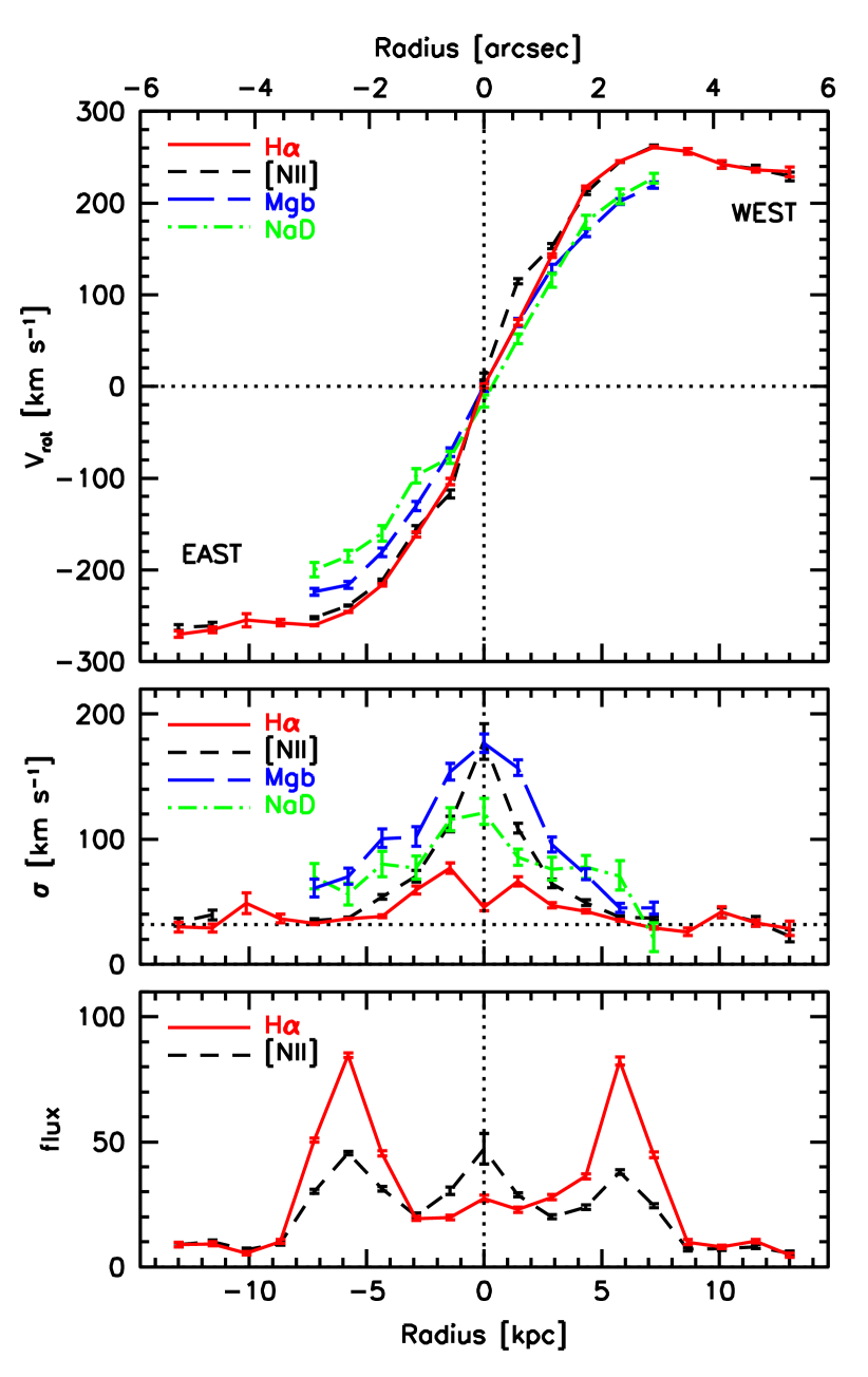
Figure 8: Rotation curve (upper panel), velocity dispersion profile (middle panel), and line flux profile for SDSS J2141$-$0001.

6.3 The rotation curve likelihood

For a given set of mass model parameters $\boldsymbol{\theta}_{\rm m}$ we can predict the circular velocity of the stars at each radius, and hence find parameter vectors that fit the rotation curve data. To do this we need to fold in the effects of beam-smearing; our procedure for this is described in the next section. We compare the predicted data ${\mathbf{v}^{\rm p}}$ and the observed data in the usual way. We assume uncorrelated Gaussian errors on the observed velocities $v_{j}$ $\sigma_{j}=\sqrt{K\sigma_{0,j}+\sigma_{\rm extra}^{2}}$ (where $\sigma_{0,j}$ are the reported error bars, and $K$ and $\sigma_{\rm extra}$ are free parameters allowing the true uncertainties to be inferred), and hence construct the familiar likelihood function

$${\rm Pr}({\mathbf{v}}|\boldsymbol{\theta}_{\rm m})=\frac{\exp{\left(-\frac{\chi_{v}^{2}}{2}\right)}}{\prod_{j=1}^{n}\sigma_{j}\sqrt{2\pi}}$$ (20)

where the misfit function

$$\chi_{v}^{2}=\sum_{j}\frac{\left(v_{j}-v^{\rm p}_{j}\right)^{2}}{\sigma_{j}^{2}}.$$ (21)

We then take the product of this likelihood and the prior PDFs on the parameters defined in Section 4 to obtain the posterior PDF for the model parameters given the kinematics data.

6.4 Modelling beam-smearing

The rotation curve data presented in Figure 9 are the observed values, uncorrected for inclination, finite slit width and seeing effects. We refer to these combined effects as beam-smearing. Since the disk inclination is high, the $\sin i$ correction is small, just a factor of $1.021$. However, since the slit width covers a large fraction of the minor axis of the galaxy, the effects of finite slit width and seeing are likely to be significant, especially near the centre of the galaxy. We take this into account when computing the predicted data ${\mathbf{v}^{\rm p}}$ as the inclined, beam-smeared, model rotation curve within a 1 arcsec slit. For computational efficiency we estimate the beam-smearing effect using a simplified, rotating exponential disk model, and then apply this correction to the model rotation curve. The intrinsic rotation curve $\hat{\mathbf{v}}$ is given by the sum of the bulge, disk and halo components as described above.

The beam-smearing calculation is approximate, because we don’t know the exact distribution of the H$\alpha$ emission, only the starlight. While we model the H$\alpha$ distribution with an exponential profile, with the scale length of the V-band light, the actual distribution is likely to be asymmetric (due to extinction), and non-exponential (there is a ring of star formation). To minimize the impact of these uncertainties, we have excluded the inner $2$ arcsec of data in our mass models.

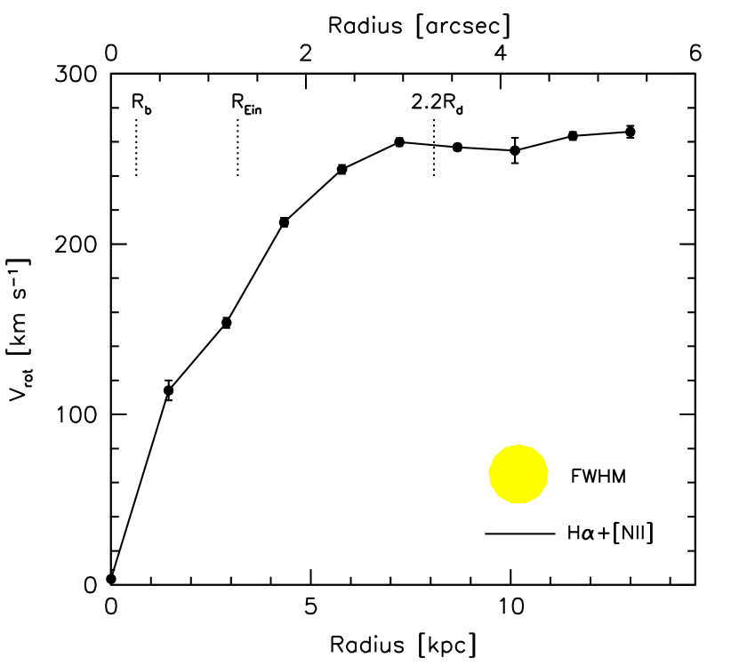
Figure 9: Folded rotation curve from emission lines of H$\alpha$ and [NII]. The location of the bulge half-light radius, $R_{\rm b}$, Einstein radius, $R_{\rm Ein}$, and 2.2 disk scale lengths, $R_{\rm d}$ are indicated with dotted lines. The spatial sampling is one point per seeing FWHM, which is indicated by the yellow circle. This rotation curve is uncorrected for inclination, and beam smearing due to the finite (1 arcsec) slit width and seeing.

Table 4: Observed Rotation Curve from Emission Lines

Radius	Radius	Rotation Velocity	Error
$[\rm arcsec]$	$[{\rm kpc}]$	$[\,\rm km\,s^{-1}]$	$[{\,\rm km\,s^{-1}}]$
0.000	0.00	3.5	5.3
0.593	1.45	114.1	5.8
1.185	2.89	153.8	2.9
1.778	4.33	212.7	2.6
2.370	5.78	243.8	2.6
2.963	7.22	259.8	2.3
3.555	8.67	256.8	2.0
4.148	10.11	254.9	7.5
4.740	11.56	263.4	2.3
5.333	13.00	265.9	3.5

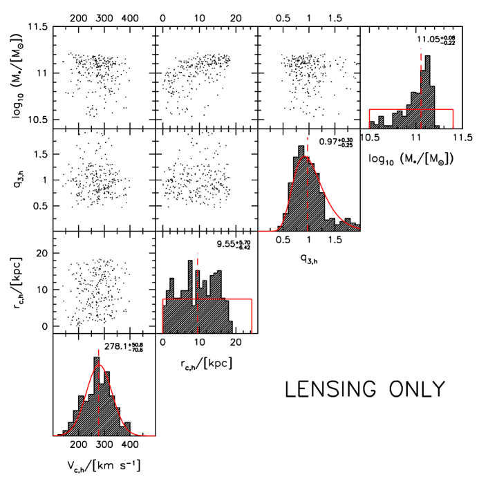
Figure 10: Marginalised two-dimensional posterior PDFs for unconstrained mass model parameters (see Table 3) using constraints from strong lensing alone. In the histogram panels, the vertical red lines show the median value. The median value together with the offsets to the 84th and 16th percentiles of the distribution is given in the top right corner. The priors are shown with solid red lines.

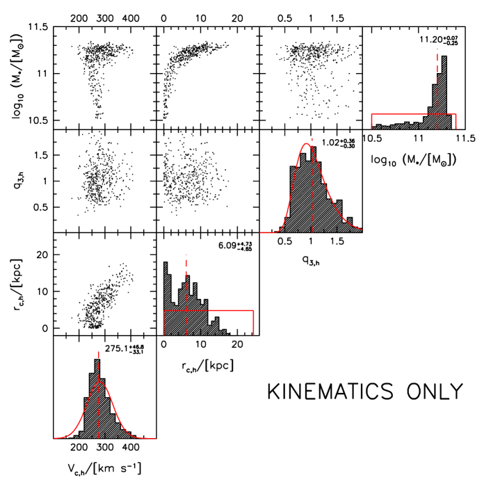
Figure 11: Marginalised two-dimensional posterior PDFs for unconstrained mass model parameters (see Table 3) using constraints from kinematics alone. In the histogram panels the vertical red lines show the median value. The median value together with the offsets to the 84th and 16th percentiles of the distribution is given in the top right corner. The priors are shown withe solid red lines.

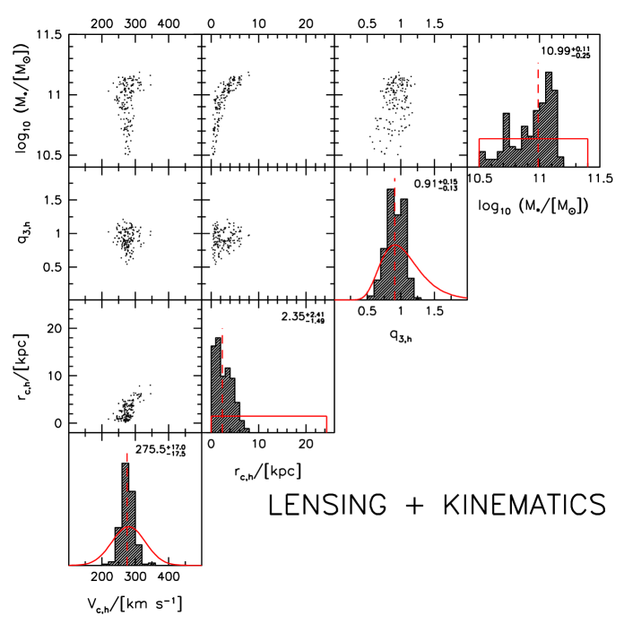
Figure 12: Marginalised two-dimensional posterior PDFs for unconstrained mass model parameters (see Table 3) using constraints from both kinematics and strong lensing. In the histogram panels the vertical red lines show the median value. The median value together with the offsets to the 84th and 16th percentiles of the distribution is given in the top right corner. The priors are shown with solid red lines.

6.5 The central velocity dispersion

The spectral line fits described in the previous section also yield some information on the velocity dispersion of the system. The central (within 1”) velocity dispersion from the Mg b–[Fe ii] lines was found to be $\sigma=180\pm 4\,\rm km\,s^{-1}$, in agreement with the SDSS value (which is integrated over the 3” fibre aperture). Na D gives a lower central velocity dispersion, of $\sigma=119\pm 6\,\rm km\,s^{-1}$. Absorption in Na D can come from interstellar gas, as well as stars. Since SDSS J2141$-$0001 has a dusty gas disk, it is thus likely that the Na D line is not reliably tracing the stellar velocity dispersion. For the emission lines the central (within the inner $0.25^{\prime\prime}$) velocity dispersion of the N ii line is $\sim 178\pm 14\,\rm km\,s^{-1}$, similar to that of the stars. However, the velocity dispersion of the N ii line declines faster with radius than that of the stars (middle panel of Figure 8). This is an indication that the peak in velocity dispersion in N ii is due to beam-smearing. For the H$\alpha$ line the central velocity dispersion is considerably lower than that of N ii, which we ascribe to the presence of absorption, which we have not corrected for. In the outer part of the disk, the observed velocity dispersion of the emission lines is close to that of the instrumental resolution of $\sim 32\,\rm km\,s^{-1}$ (dotted horizontal line in middle panel of Figure 8), indicating that the intrinsic velocity dispersion of the line-emitting gas disk is too low to be resolved.

How could we model the velocity dispersion data? Our simple dynamical model does not easily allow for this, but we can make use of the dispersion information as a cross-check in the following simplistic way. The results of Padmanabhan et al. (2004) and Wolf et al. (2010) show that, for a spherical system, the circular velocity at the half-light radius $V_{\rm circ}(R_{\rm 50})\simeq 1.7\sigma_{\rm los}$, where $\sigma_{\rm los}$ is the integrated line of sight velocity dispersion of the system. For the case of SDSS J2141$-$0001, the bulge half light radius is $R_{\rm 50,b}\simeq 0.26"$, and thus the integrated velocity dispersion within the inner $1"$ gives the integrated velocity dispersion of the bulge.

Applying the $V_{\rm circ}$ formula above and adopting an uncertainty of 10% results in an estimate of the circular velocity at $R_{\rm 50}$ of $V_{\rm circ}(R_{50,\rm b})=306\pm 31\,\rm km\,s^{-1}$. In our current analysis we do not make use of this constraint. Rather, we use this as a consistency check to our models which are constrained by strong lensing and gas rotation curve.

7 Results

We now infer the parameters of our 3-component mass model using constraints from the strong lensing and kinematics data presented in the previous two sections. In order to sample the posterior distribution for the parameters we use the Diffusive Nested Sampling code from Brewer et al. (2009). Diffusive Nested Sampling is a powerful and efficient alternative to standard MCMC sampling.

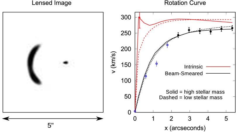
Figure 13: Example mass model that fits the lensing (left panel) and kinematics (right panel) data. In the right panel two models are shown: median stellar mass (solid lines); low stellar mass (dashed lines). The red lines show the intrinsic model circular velocity, while the black lines show the model circular velocity after beam-smearing, finite slit width, and inclination effects are taken into account. Only the black points beyond 2 arcsec are included in the fit. The red point at small radii is the constraint from the stellar velocity dispersion, and disfavors the low stellar mass solution.

7.1 Inferred Model Parameters

We consider inferences from three data sets:

1. strong lensing only

2. kinematics only

3. strong lensing plus kinematics

In Figures 10–12 we plot, for each data set, all possible one-dimensional and two-dimensional marginalised posterior PDFs for the four main mass model parameters. These parameters are the total (disk+bulge) stellar mass $M_{*}$, and the dark matter halo asymptotic circular velocity, $V_{\rm c,h}$, core radius $r_{\rm c,h}$, and 3 dimensional flattening, $q_{3,\rm h}$. The median, 16th and 84th percentiles of the marginalized posterior PDFs for these parameters individually are given in Table LABEL:tab:mm.

The constraints on stellar mass, dark halo density, and dark halo shape are discussed in more detail below. We first point out some of the main features of these figures.

With strong lensing alone (Figure 10), the halo parameters are poorly constrained: The PDF for the core radius is almost uniform, while the PDFs for the halo velocity and halo axis ratio follow the priors. This is expected owing to the limited range in projected radius probed by the lensing constraints. There is, however, a good constraint on the stellar mass: $\log_{10}(M_{*}/{\rm M_{\odot}})=11.05^{+0.08}_{-0.22}$. This is a result of the axis ratio of the projected mass being quite low (§5.2).

With kinematics alone (Figure 11), the halo core radius is slightly better constrained, and the stellar mass is less well constrained. There is a strong degeneracy between the halo core radius and the stellar mass, with higher stellar masses requiring higher core radii — this is the classic disk-halo degeneracy. Related to this there is a degeneracy between halo velocity and core radius, with higher halo velocities requiring larger core radii.

Table 5: Summary of fitted parameters: stellar mass ($M_{*}$); halo asymptotic circular velocity ($v_{\rm c,h}$); halo core radius ($r_{\rm c,h}$); and 3D halo axis ratio ($q_{3,\rm h}$).

	$\log_{10}(M_{*}/{\rm M_{\odot}})$	$V_{\rm c,h}/[\,\rm km\,s^{-1}]$	$r_{\rm c,h}/[{\rm kpc}]$	$q_{\rm 3,h}$
Lensing	$11.05^{+0.08}_{-0.22}$	$278^{+51}_{-71}$	$9.6^{+5.7}_{-6.4}$	$0.97^{+0.30}_{-0.25}$
Kinematics	$11.20^{+0.07}_{-0.25}$	$275^{+47}_{-33}$	$6.1^{+4.7}_{-4.7}$	$1.02^{+0.36}_{-0.30}$
Lensing + Kinematics	$10.99^{+0.11}_{-0.25}$	$276^{+17}_{-18}$	$2.35^{+2.4}_{-1.5}$	$0.91^{+0.15}_{-0.13}$

Adding the strong lensing constraints to the kinematics constraints breaks some of the degeneracies. Specifically, it removes the highest stellar mass solutions from the kinematics only analysis. All posteriors are considerably tighter than the priors, illustrating the power of the combined analysis: for example, circular velocity is now known to 6% precision, and core radius is well constrained to be smaller than 5 kpc. However, there is still a degeneracy between halo core radius and stellar mass. There is also a residual degeneracy between stellar mass and halo shape — with low stellar mass solutions favoring oblate dark matter haloes. This degeneracy is expected as the total mass needs to be flattened to reproduce the strong lensing (Section 5.2). The flattening can be achieved with either a significant stellar disk component and a spherical halo, or a less massive disk and a more flattened halo.

In Figure 13 we show the rotation curves and strong lensing image predicted by two example mass models drawn from the posterior PDF given both lensing and kinematics data. These models both predict four images of the lensed source, including a faint counter-image that is consistent with the noise in the centre of the subtracted image. Both models’ predicted rotation curves fit the outer part of the observed rotation curve very well; they also match well the central part of the observed rotation curve, which was not used in the fit. The two models have either the posterior median stellar mass, or much lower stellar mass; they can only be distinguished in the plot of the intrinsic, pre beam-smeared rotation curves, where the high stellar mass model has a significantly higher rotation velocity at radii less than one arcsec. This region could be probed with higher spatial resolution spectroscopy, or by making use of the velocity dispersion information. Indeed, our cross-check point from Section 6.5 would favour the high stellar mass model.

In Figure 14 we show the inferred circular velocity profile, decomposed into baryonic and dark matter components. These estimates are based on the posterior samples using the joint lensing plus kinematics analysis. The solid lines show the median model from the posterior PDF, while the shaded regions enclose 68% of the models. In the radial region where we have observational constraints (i.e., from the Einstein radius to the last rotation curve point) the total circular velocity is well constrained. For example, at 2.2 disk scale lengths (8.1 kpc), the total circular velocity is $V_{2.2}=289\pm 4\,\rm km\,s^{-1}$. The circular velocity profiles of the baryons and dark matter are not as tightly constrained. Nevertheless, we can still infer interesting constraints on the dark matter fraction as a function of radius, and thus determine whether or not SDSS J2141$-$0001 has a maximum disk. A working definition of a maximum disk is when $V_{\rm disk}(2.2R_{\rm d})/V_{\rm tot}(2.2R_{\rm d})=0.85\pm 0.10$ (Sackett 1997). Here $V_{\rm disk}(2.2R_{\rm d})$ is the circular velocity of the disk at 2.2 disk scale lengths, and $V_{\rm tot}(2.2R_{\rm d})\equiv V_{2.2}$ is the total circular velocity at 2.2 disk scale lengths.

A galaxy may have a sub-maximal disk, but still have a maximal baryonic component due to the bulge. Thus we consider the contribution of the baryons (i.e., bulge plus disk) to $V_{2.2}$ to be of more relevance than just the contribution of the disk to $V_{2.2}$. We find that $V_{\rm bar}(2.2R_{\rm d})/V_{2.2}=0.67^{+0.10}_{-0.17}$, which suggests that SDSS J2141$-$0001 is sub-maximal at 2.2 disk scale lengths. However, the baryon contribution to the total circular velocity increases towards smaller radii (lower panel of Fig. 14) such that $V_{\rm bar}(R_{\rm b})/V_{\rm tot}=0.99^{+0.01}_{-0.09}$, and thus SDSS J2141$-$0001 is maximal at the bulge half-light radius. Converting circular velocities into spherical masses, results in a dark matter fraction of $f_{\rm DM}=0.55^{+0.20}_{-0.15}$ within 2.2 disk scale lengths, and $f_{\rm DM}=0.02^{+0.17}_{-0.02}$ within the bulge half-light radius.

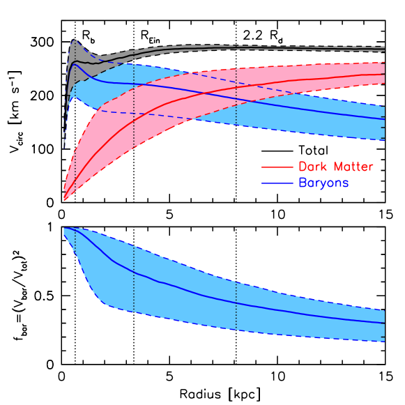
Figure 14: Circular velocity profiles (upper panel) and spherical baryon fractions (lower panel) from our joint lensing plus kinematics analysis. The solid lines show the median, while the shaded regions enclose 68% of the posterior PDF. The total circular velocity (black line and grey shaded region) is well constrained outside of the Einstein radius, $R_{\rm Ein}$, and up to the last rotation curve point at 13 kpc. The contributions of the baryons (red lines and shaded regions) and the dark matter (blue lines and shaded regions) are more uncertain. However, at the bulge half-light radius, $R_{b}$, the galaxy is baryon dominated (and thus is “maximal”), while at 2.2 disk scale lengths the baryons fraction is roughly 50% (and thus is “sub-maximal”).

7.2 Constraints on the stellar IMF

Figure 15 shows the posterior PDFs from our joint lensing and kinematics analysis together with those from SPS models for both Chabrier and Salpeter IMFs. From our lensing and kinematics analysis the stellar mass of the galaxy is found to be $\log_{10}M_{*}=10.99^{+0.11}_{-0.25}$. This is in excellent agreement with the stellar mass derived from SED fitting assuming a Chabrier IMF, which is $\log_{10}M_{*}=10.97\pm{0.07}$. A Salpeter IMF results in stellar masses 0.24 dex higher. Our analysis thus mildly favors a Chabrier IMF over a Salpeter IMF. We can quantify this agreement by integrating the likelihood over a prior for the stellar mass defined by either the Chabrier or the Salpeter SPS model PDFs. The ratio of these integrals is the Bayes factor, or evidence, in favour of a Chabrier IMF; we find its value to be 2.7, which is to say that the data are 2.7 times more likely to have come from the Chabrier model than from the Salpeter one. If these are the only two models possible, then there is a 73% chance that the Chabrier model is the true one. This corresponds to weak evidence in favor of Chabrier vs Salpeter.

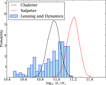
Figure 15: Inference on stellar mass from lensing and kinematics (histogram) compared with SPS models (solid lines) assuming a Chabrier IMF (black) and Salpeter IMF (red). The Bayes factor in favor of a Chabrier IMF, compared to a Salpeter IMF is 2.5.

In our current analysis we ignore the possibility of cold gas. For massive spiral galaxies the cold gas fraction is $\simeq 20\pm 10\%$ (assuming a Chabrier IMF), split roughly equally between atomic and molecular gas (e.g., Dutton & van den Bosch 2009). If the cold gas is distributed like the stars, then the lensing+kinematics stellar mass is actually a baryonic mass, greater than or equal to the actual stellar mass. If the cold gas is more extended than the stars, as is often the case, then we will still be over-estimating the stellar mass, but by a smaller amount. To estimate an upper limit to the impact of cold gas on our derived stellar masses we assume that the gas mass for SDSS J2141$-$0001 is distributed like the stars. For each model in the posterior PDF we draw a gas mass from a log-normal distribution centered on $M_{\rm gas}=1.8\times 10^{10}{\rm M_{\odot}}$, with a standard deviation of 0.3 dex. We then subtract off the gas mass from the gas free stellar mass to derive the “true” stellar mass. The results of this exercise are shown in Fig. 16. The resulting median and 68% confidence interval on the stellar mass is $\log_{10}(M_{*}/{\rm M_{\odot}})=10.89^{+0.15}_{-0.33}$, i.e., 0.1 dex lower than when ignoring the cold gas. The Bayes factor in favor of a Chabrier IMF over a Salpeter IMF has increased from 2.7 to 11.9, which corresponds to strong evidence. Thus by ignoring the cold gas we could be over estimating the stellar mass by $\simeq 0.1\pm 0.05$ dex, which strengthens the case for an IMF lighter than Salpeter.

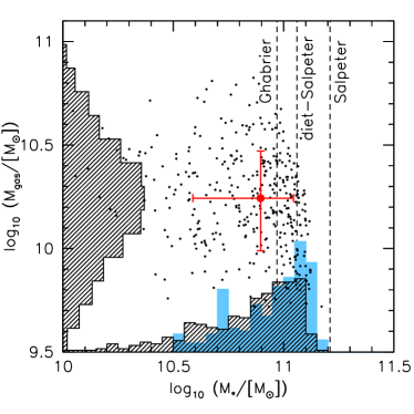
Figure 16: Effect of gas mass on the inferred stellar mass from lensing and kinematics. For each model galaxy in the posterior PDF we draw a gas mass from a log-normal distribution with mean and standard deviation typical for massive spiral galaxies. The resulting PDFs for the stellar and gas mass are shown as black hatched histograms. For comparison, the blue shaded histogram shows the posterior PDF on the stellar mass assuming no gas mass. Thus accounting for cold gas mass reduces the stellar mass derived from lensing and kinematics by $\simeq 0.1$ dex.

How does this result compare to previous work? Using maximal disk fits to spiral galaxy rotation curves in the Ursa Major cluster, Bell & de Jong (2001) placed an upper limit on the stellar mass-to-light ratio normalisation, favoring IMFs with stellar masses 0.15 dex lower than Salpeter, the so-called diet-Salpeter IMF. We note that a Salpeter IMF is also disfavored for fast rotating elliptical galaxies (Cappellari et al. 2006; Treu et al. 2010; Auger et al. 2010; Barnabé et al. 2010), but is favored for massive elliptical galaxies (Treu et al. 2010; Auger et al. 2010; van Dokkum & Conroy 2010). Thus comparing our result with those for massive ellipticals, supports the idea that the IMF is not universal, but dependent on galaxy mass and/or Hubble type.

By shifting our Salpeter stellar mass PDF by $-0.15$ dex, we find that for SDSS J2141$-$0001 a diet Salpeter IMF corresponds to a stellar mass of $\log_{10}(M_{*}/{\rm M_{\odot}})=11.06\pm{0.07}$. This IMF is favored over a Salpeter IMF, by Bayes factors of 3.5 (assuming no cold gas), and 9.9 (assuming a gas mass of $\log_{10}(M_{\rm gas}/{\rm M_{\odot}})=10.26\pm 0.30$). There is little evidence distinguishing between diet Salpeter and Chabrier IMFs.

7.3 Constraints on the dark halo density profile

N-body simulations have shown that in $\Lambda$CDM cosmologies dark matter haloes are expected (in the absence of baryonic effects) to have very specific structure. The mass density profiles can be well approximated by the so called NFW profile (Navarro et al. 1997). This has a density profile that varies from $\rho(r)\propto r^{-1}$ at small radii, to $\rho\propto r^{-3}$ at large radii. The radius where the logarithmic slope of the density profile is ${\rm d}\ln\rho/{\rm d}\ln r=-2$ is known as the scale radius, $r_{\rm s}$. The halo scale radii are tightly correlated with the virial masses of dark matter haloes, $M_{\rm vir}$. This correlation is usually expressed in terms of the halo concentration, $c=r_{\rm vir}/r_{\rm s}$, where $r_{\rm vir}$ is the virial radius. Halo concentrations are only weakly dependent on halo mass, with a relation of the form $c\propto M_{\rm vir}^{-0.1}$ (Macció et al. 2007). The scatter in halo concentration, at fixed halo mass, for relaxed haloes is small $\simeq 0.11$ dex (Jing 2000; Wechsler et al. 2002; Macció et al. 2007).

Observationally, measuring halo concentrations is a challenge because halo virial masses are poorly constrained for individual galaxies, due to the lack or sparsity of dynamical tracers at large radii. A more observationally accessible measure of dark halo structure is the parameter $\Delta_{V/2}$, which depends on the maximum halo circular velocity, $V_{\rm max}$, and the radius where circular velocity of the halo is half of the maximum, $r_{V/2}$ (Alam, Bullock & Weinberg 2002):

$$\Delta_{V/2}=5\times 10^{5}\left(\frac{V_{\rm max}/[100\,\rm km\,s^{-1}]}{r_{V/2}/[h^{-1}{\rm kpc}]}\right)^{2}.$$ (22)

For NFW haloes there is a one-to-one mapping between $\Delta_{V/2}-V_{\rm max}$ and $c-M_{\rm vir}$, and thus one can compare the observed $\Delta_{V/2}$ with predictions for $\Lambda$CDM haloes. Figure 17 shows the predictions for $\Delta_{V/2}-V_{\rm max}$ in a WMAP 5th year cosmology (Dunkley et al. 2009) from Macciò, Dutton, & van den Bosch (2008). The shaded regions show the 1 and 2$\sigma$ intrinsic scatter. The large symbols show measurements from dwarf and low surface brightness galaxies after subtracting of the baryons (de Blok et al. 2001; de Blok & Bosma 2002; Swaters et al. 2003). These are in excellent agreement with the predictions from $\Lambda$CDM.

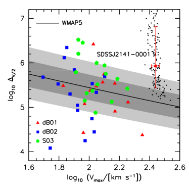
Figure 17: Central density of the dark matter halo, $\Delta_{V/2}$ vs maximum halo circular velocity, $V_{\rm max}$. The solid black line shows the prediction for pristine dark matter haloes in the concordance $\Lambda$CDM cosmology (WMAP5) from Macciò et al. (2008). The shaded regions show the 1 and $2\sigma$ intrinsic scatter. The colored symbols show measurements from dwarf and low surface brightness galaxies, after subtraction of the baryons (de Blok et al. 2001, dB01; de Blok & Bosma 2002, dB02; Swaters et al. 2003, S03). The small black dots show samples from the posterior PDF for SDSS J2141$-$0001. The large red dot and error bars show the median and 68% ranges of this PDF, respectively.

In our mass model of SDSS J2141$-$0001, the dark matter halo has a softened isothermal density profile, which has $V_{\rm max}=V_{\rm c,h}$, and $r_{V/2}=1.1263\,r_{\rm c,h}$. We can compute $\Delta_{V/2}$ for this model and compare it with the NFW profile halos of the simulations. For our model the median and uncertainty (corresponding to 16th and 84th percentiles) is $\log_{10}\Delta_{V/2}=5.9^{+0.9}_{-0.5}$. The median is $2.7\sigma$ higher (in terms of intrinsic scatter) than that predicted for pristine $\Lambda$CDM haloes, although the full posterior PDF overlaps the $\Lambda$CDM predictions, as shown in Figure 17. The 16th percentile of the PDF for $\Delta_{V/2}$ only corresponds to a $1.1\sigma$ deviation from the $\Lambda$CDM distribution. Thus there is a suggestion that the SDSS J2141$-$0001 halo is higher density than expected. We note that, as shown in Fig. 18, the central density is highly correlated with the stellar mass, with lower $\Delta_{V/2}$ for higher $M_{*}$.

There are two interpretations of the higher than expected halo density. 1) The halo has undergone contraction in response to galaxy formation (e.g., Blumenthal et al. 1986). 2) The halo of SDSS J2141$-$0001 has a higher density than typical haloes of the same mass. In order to distinguish between these two scenarios it is necessary to understand the selection function of the SWELLS lens galaxies. We cannot do this with one galaxy, and therefore we will leave this for future work. Nevertheless, we can gain some insight by investigating where SDSS J2141$-$0001 falls on disk galaxy scaling relations.

We consider the relations between stellar mass ($M_{*}$), rotation velocity at 2.2 disk scale lengths ($V_{2.2}$), and disk scale length ($R_{\rm d}$). For SDSS J2141$-$0001 the values of these parameters are $V_{2.2}\simeq 289\,\rm km\,s^{-1}$, $\log_{10}(M_{*,\rm Chab}/{\rm M_{\odot}})\simeq 11.0$, and $R_{\rm d}\simeq 3.7{\rm kpc}$. For a stellar mass of $10^{11}{\rm M_{\odot}}$ we expect $V_{2.2}=229\pm 25\,\rm km\,s^{-1}$ (Dutton et al. 2010b). Alternatively, for a rotation velocity of $V_{2.2}=289\,\rm km\,s^{-1}$ we expect a stellar mass of $\log_{10}(M_{*}/{\rm M_{\odot}})=11.39^{+0.18}_{-0.18}$, assuming a Chabrier IMF. For a rotation velocity of $V_{2.2}=289\,\rm km\,s^{-1}$ we expect $R_{\rm d}=6.0^{+2.7}_{-1.9}{\rm kpc}$ (Courteau et al. 2007; Dutton et al. 2007). Thus SDSS J2141$-$0001 is offset to low stellar mass (by $\simeq 2\sigma$ and small size (by $\simeq 1.3\sigma$) at fixed rotation velocity, which means that it has a higher baryonic and total mass density than typical massive spiral galaxies.

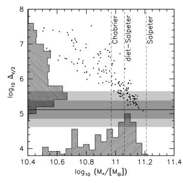
Figure 18: Central density of the dark matter halo, $\Delta_{V/2}$ vs stellar mass, $M_{*}$. The solid black line shows the prediction for pristine dark matter haloes in the concordance $\Lambda$CDM cosmology (WMAP5). The shaded regions show the 1 and $2\sigma$ intrinsic scatter. The black dots show samples from the posterior PDF for SDSS J2141$-$0001. The maximum likelihood stellar masses from SPS models assuming Chabrier, diet-Salpeter, and Salpeter IMFs are shown with vertical dashed lines.

The high central density of SDSS J2141$-$0001 may be related to how it was selected. If the central densities of spiral galaxies are close to the critical value for strong lensing, then the galaxies that are observed to be strong lenses could be a biased sub-set of the population. Thus the conclusions we draw for SDSS J2141$-$0001 might not necessarily be applicable to spiral galaxies in general. This selection effect is likely to affect the interpretation of some parameters more than others. For example, in order to interpret the central densities of dark matter haloes in terms of the halo response to galaxy formation it is necessary for the lenses to reside in an unbiased subset of haloes. However, if we assume that the IMF is universal, at least for massive spiral galaxies, then the constraints we place on the IMF using spiral galaxy strong lenses will be independent of any selection bias. Larger samples of spiral galaxy lenses are obviously needed to fully characterise the selection biases in spiral galaxy lenses.

7.4 Constraints on the dark halo shape

N-body simulations have shown that in $\Lambda$CDM cosmologies dark matter haloes are triaxial, with a preference towards prolate shapes (Jing & Suto 2002; Bailin & Steinmetz 2005; Kasun & Evrard 2005; Allgood et al. 2006; Bett et al. 2007; Macciò et al. 2007, 2008). For a halo mass of $M_{\rm vir}=10^{12}{\rm M_{\odot}}$, which is typical for massive spiral galaxies, the minor to major axis ratio ratio $c/a\simeq 0.63\pm 0.1$, and the intermediate to major axis ratio $b/a\simeq 0.80\pm 0.1$ (Macciò et al. 2008). $\Lambda$CDM haloes are also found to be more prolate at smaller radii (Allgood et al. 2006; Macciò et al. 2008; Abadi et al. 2010) .

The assembly of a central galaxy is expected to modify the three dimensional shape of the dark matter halo (Katz & Gunn 1991; Dubinski 1994). Using cosmological simulations Abadi et al. (2010) found that as a result of the assembly of the central galaxy the haloes become nearly oblate with $b/a\simeq 0.95$ and $c/a\simeq 0.85$, and the axial ratios become approximately independent of radius. Similar results have been obtained from other cosmological simulations (e.g., Tissera et al. 2010). It should be noted that these simulations over-predict the baryon to dark halo mass ratios, and thus the effect of galaxy assembly on the halo shapes could be over-estimated.

In our mass models we assume the halo is axisymmetric, with 3D axis ratio $q_{3,\rm h}$. A spherical halo has $q_{3,\rm h}=1$, an oblate halo has $q_{3,\rm h}<1$, and a prolate halo has $q_{3,\rm h}>1$. We adopt a log-normal prior on the halo axis ratio, centered on $q_{3,\rm h}=1$. For our fits to lensing only or kinematics only the posterior PDF for $q_{3,\rm h}$ is identical to the prior, but for the joint analysis slightly oblate haloes are preferred: $q_{3,\rm h}=0.91^{+0.15}_{-0.13}$, and prolate haloes with $q_{3,\rm h}>1.2$ are strongly disfavored. Thus our results for SDSS J2141$-$0001 support the notion that galaxy assembly sphericalizes the dark matter halo, and perhaps even flattens it towards the disk.

8 Conclusions

We have presented an analysis of the strong gravitational lens SDSS J2141$-$0001, discovered as part of the SLACS survey, using data from HST and the Keck telescopes. The lens galaxy is a high inclination disk dominated galaxy with $K^{\prime}$-band bulge fraction of 0.2, showing stellar rotation in multiple spectral lines. A singular isothermal ellipsoid lens model provides a circular velocity of $V_{\rm c}=254^{+15}_{-18}\,\rm km\,s^{-1}$ and an axis ratio of $q=0.42^{+0.17}_{-0.12}$.

We perform a joint fit to the multi-filter surface brightness, lensing and kinematics data using a self-consistent 3-component mass model, and from it draw the following conclusions:

• The lensing and kinematics constraints yield a stellar mass of $\log_{10}(M_{*}/{\rm M_{\odot}})=10.99^{+0.11}_{-0.25}$ (68% confidence interval), independent of the IMF.

• This value is in excellent agreement with the stellar mass derived from the SED using SPS models and assuming a Chabrier (2003) IMF: $\log_{10}(M_{*}/{\rm M_{\odot}})=10.97^{+0.07}_{-0.07}$. A Salpeter (1955) IMF results in stellar masses 0.24 dex higher: our analysis marginally favors a Chabrier IMF over a Salpeter IMF, by a Bayes factor of 2.7.

• Accounting for the expected gas mass reduces the lensing and kinematics stellar mass by $0.10\pm 0.05$ dex, and increases the Bayes factor in favor of a Chabrier IMF to 11.9.

• At 2.2 disk scale lengths the spherical dark matter fraction is $f_{\rm DM}=0.55^{+0.20}_{-0.15}$, suggesting that the baryons are sub-maximal.

• The dark matter halo has a maximum circular velocity of $V_{\rm c,h}=276^{+17}_{-18}\,\rm km\,s^{-1}$, and a core radius of $r_{\rm c,h}=2.4^{+2.4}_{-1.5}{\rm kpc}$. The corresponding central density parameter $\log_{10}\Delta_{V/2}=5.9^{+0.9}_{-0.5}$ is higher than expected for uncontracted NFW haloes in the concordance $\Lambda$CDM cosmology, which have $\log_{10}\Delta_{V/2}=5.2$ and an intrinsic scatter of 0.3.

• This high density could either be evidence for halo contraction in response to galaxy formation (e.g., Blumenthal et al. 1986), or the result of a selection bias towards high concentration haloes. A larger sample with well-characterised selection function is required to make further progress.

• The dark matter halo is oblate, $q_{3,\rm h}=0.91^{+0.15}_{-0.13}$, with a probability of 69%. This finding provides support for the notion that galaxy assembly turns strongly prolate triaxial dark matter haloes into roughly oblate axisymmetric haloes (e.g., Abadi et al. 2010).

Appendix A The Chameleon approximation to a Sérsic Profile

In this appendix we derive an approximation to a Sérsic profile as the difference of two non-singular isothermal ellipsoids (NIE’s).

The Sérsic profile is specified by three parameters: a normalization, a radial scale, and a shape parameter commonly known as the Sérsic index, $n$. In its simplest form it is given by:

$$\Sigma(R)=\Sigma_{0}\exp\left[-\left(\frac{R}{R_{\rm 0}}\right)^{1/n}\right]$$ (23)

where $\Sigma_{0}$ is the central surface density, and $R_{0}$ is the radial scale. The Sérsic profile is commonly expressed in terms of the effective radius, $R_{\rm e}$, which encloses half of the projected mass, and the effective density, $\Sigma_{\rm e}\equiv\Sigma(R_{\rm e})$:

$$\Sigma(R)=\Sigma_{\rm e}\exp\left\{-b_{n}\left[\left(\frac{R}{R_{\rm e}}\right)^{1/n}-1\right]\right\}.$$ (24)

Where the term $b_{n}\approx 2n-0.32$. Here we use the asymptotic expansion of Ciotti & Bertin (1999) to $O(n^{-5})$ valid to one part in $\sim 10^{4}$ for $n>0.36$:

$$b_{n}=2n-\frac{1}{3}+\frac{4}{405n}+\frac{46}{25515n^{2}}+\frac{131}{1148175n^{3}}$$

$$-\frac{2194697}{30690717750n^{4}}+O(n^{-5}).$$ (25)

Equation 23 and Equation 24 are related to each other via

$$R_{\rm e}=(b_{n})^{n}R_{0}$$ (26)

and

$$\Sigma_{\rm e}=\exp(-b_{n})\Sigma_{0}.$$ (27)

The Chameleon profile is the difference between two NIEs with different core radii, but the same normalization (which insures the total mass is finite):

$$\Sigma_{\rm chm}(R;\Sigma_{1},R_{1},R_{2})=$$

$$\left(\frac{\Sigma_{1}}{\sqrt{R^{2}+R_{1}^{2}}}-\frac{\Sigma_{1}}{\sqrt{R^{2}+R_{2}^{2}}}\right).$$ (28)

For the purpose of comparing to a Sérsic profile, we use the following parametrization.

$$\Sigma_{\rm chm}(R;\Sigma_{0},R_{0},\alpha)=$$

$$\frac{\Sigma_{0}}{1-\alpha}\left(\frac{R_{0}}{\sqrt{R^{2}+R_{0}^{2}}}-\frac{R_{0}}{\sqrt{R^{2}+(R_{0}/\alpha)^{2}}}\right).$$ (29)

Where $\Sigma_{0}=\Sigma_{1}(1-\alpha)/R_{1}$ is the central surface density of the chameleon profile, $R_{0}=R_{1}$, and $\alpha$ is the ratio between the core radii of the two NIE’s: $\alpha=R_{1}/R_{2}$, so that $0<\alpha<1$. The total mass of the Chameleon profile is

$$M_{\rm Chm}=\pi\Sigma_{0}R_{0}^{2}/\alpha.$$ (30)

We wish to find the correspondence between the Sérsic parameters, $\Sigma_{0,\rm Ser}$, $R_{0,\rm Ser}$, $n_{\rm Ser}$, and the Chameleon parameters, $\Sigma_{0,\rm Chm}$, $R_{0,\rm Chm}$, $\alpha_{\rm Chm}$. We do this by fitting a Chameleon profile to a Sérsic profile. We are interested in mass profiles, so we fit $R\,\Sigma(R)$ to give appropriate weight to the density profile at large radii. Figure 19 shows the best fit parameters as a function of Sérsic index. We fit these relations between chameleon and Sérsic parameters with a cubic function:

$$y=y_{0}+y_{1}(x-x_{0})+y_{2}(x-x_{0})^{2}+y_{3}(x-x_{0})^{3}$$ (31)

The parameters of these fits are given in Table LABEL:tab:chmserfit. Our fitting function is valid for $1\leq n_{\rm Ser}\leq 4$.

Figure 19: Relation between Chameleon and Sérsic parameters as a function of Sérsic index.

Figure 20 shows Chameleon fits to Sérsic profiles with Sérsic index $n=1,2,3,$ & $4$ using the fitting function in Table LABEL:tab:chmserfit. The left panels show $\log_{10}\Sigma(R)$ vs $(R/R_{\rm e})^{1/n}$. In these units Sérsic profiles are straight lines. The Chameleon profiles deviate most significantly from Sérsic profiles at small radii, where the Chameleon profile has a constant density core. The middle panels show $R\Sigma(R)$ vs $R/R_{\rm e}$, which are the curves that were fitted against. The right panels show the cumulative mass profile. For radii between $0.5\mathrel{\hbox to0.0pt{\lower 3.0pt\hbox{$\sim$}\hss}\raise 2.0pt\hbox{$<$}}R\mathrel{\hbox to0.0pt{\lower 3.0pt\hbox{$\sim$}\hss}\raise 2.0pt\hbox{$<$}}3.0$ effective radii the mass residuals are only a few percent, and thus for most strong lensing and dynamical purposes the Chameleon approximation to a Sérsic profile is of sufficient accuracy.

Table 6: Parameters of cubic fitting formula (Equation 31) to the relations in Figure 19.

$x$	$y$	$x_{0}$	$y_{0}$	$y_{1}$	$y_{2}$	$y_{3}$
$n$	$\log_{10}\left(\frac{\Sigma_{0,\rm Chm}}{\Sigma_{0,\rm Ser}}\right)$	1.69	-0.254	-0.259	-0.036	0.014
$n$	$\log_{10}\left(\frac{R_{0,\rm Chm}}{R_{0,\rm Ser}}\right)$	1.15	0.078	-0.184	0.473	-0.079
$n$	$\log_{10}(\alpha_{\rm Chm})$	2.03	-0.739	-0.527	-0.012	-0.008

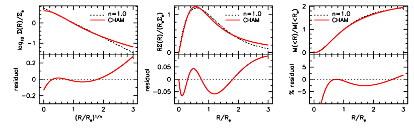
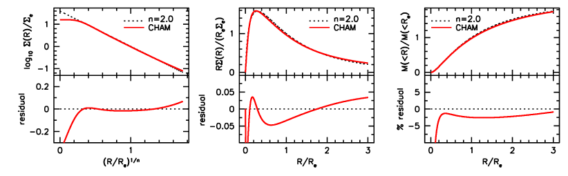
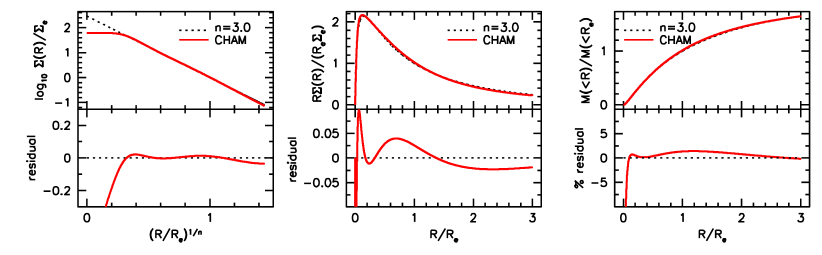
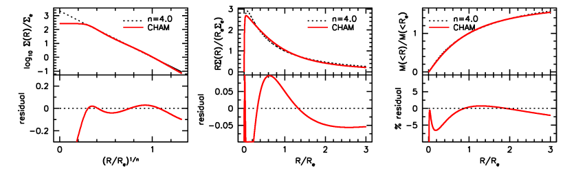
Figure 20: Chameleon fits (red solid lines) to Sérsic profiles (dotted lines) with $n=1,2,3,4$. The Chameleon profile reproduces the cumulative mass profile of a Sérsic profile to a few percent over most radii interesting for strong lensing and kinematics.

References

- (1)
- Abadi et al. (2010) Abadi, M. G., Navarro, J. F., Fardal, M., Babul, A., & Steinmetz, M. 2010, MNRAS, 407, 435
- Abazajian et al. (2009) Abazajian, K. N., et al. 2009, ApJS, 182, 543
- Alam et al. (2002) Alam, S. M. K., Bullock, J. S., & Weinberg, D. H. 2002, ApJ, 572, 34
- Allgood et al. (2006) Allgood, B., Flores, R. A., Primack, J. R., Kravtsov, A. V., Wechsler, R. H., Faltenbacher, A., & Bullock, J. S. 2006, MNRAS, 367, 1781
- Auger et al. (2009) Auger, M. W., Treu, T., Bolton, A. S., Gavazzi, R., Koopmans, L. V. E., Marshall, P. J., Bundy, K., & Moustakas, L. A. 2009, ApJ, 705, 1099
- Auger et al. (2010) Auger, M. W., Treu, T., Gavazzi, R., Bolton, A. S., Koopmans, L. V. E., & Marshall, P. J. 2010, ApJL, 721, L163
- Bailin & Steinmetz (2005) Bailin, J., & Steinmetz, M. 2005, ApJ, 627, 647
- Begeman (1987) Begeman, K. G. 1987, Ph.D. Thesis,
- Bell & de Jong (2001) Bell, E. F., & de Jong, R. S. 2001, ApJ, 550, 212
- Bershady et al. (2010) Bershady, M. A., Verheijen, M. A. W., Swaters, R. A., Andersen, D. R., Westfall, K. B., & Martinsson, T. 2010, ApJ, 716, 198
- Bett et al. (2007) Bett, P., Eke, V., Frenk, C. S., Jenkins, A., Helly, J., & Navarro, J. 2007, MNRAS, 376, 215
- Blais-Ouellette et al. (2004) Blais-Ouellette, S., Amram, P., Carignan, C., & Swaters, R. 2004, A&A, 420, 147
- Blumenthal et al. (1986) Blumenthal, G. R., Faber, S. M., Flores, R., & Primack, J. R. 1986, ApJ, 301, 27
- Bolton et al. (2006) Bolton, A. S., Burles, S., Koopmans, L. V. E., Treu, T., & Moustakas, L. A. 2006, ApJ, 638, 703
- Bolton et al. (2008) Bolton, A. S., Burles, S., Koopmans, L. V. E., Treu, T., Gavazzi, R., Moustakas, L. A., Wayth, R., & Schlegel, D. J. 2008, ApJ, 682, 964
- Bosma (1978) Bosma, A. 1978, Ph.D. Thesis,
- Bottema (1993) Bottema, R. 1993, A&A, 275, 16
- Brewer & Lewis (2006) Brewer, B. J., & Lewis, G. F. 2006, ApJ, 637, 608
- Brewer et al. (2009) Brewer, B. J., Pártay, L. B., & Csányi, G. 2009, arXiv:0912.2380
- Bullock et al. (2001) Bullock, J. S., Kolatt, T. S., Sigad, Y., Somerville, R. S., Kravtsov, A. V., Klypin, A. A., Primack, J. R., & Dekel, A. 2001, MNRAS, 321, 559
- Cappellari et al. (2006) Cappellari, M., et al. 2006, MNRAS, 366, 1126
- Carignan & Freeman (1985) Carignan, C., & Freeman, K. C. 1985, ApJ, 294, 494
- Castander et al. (2006) Castander, F. J., Treister, E., Maza, J., & Gawiser, E. 2006, ApJ, 652, 955
- Chabrier (2003) Chabrier, G. 2003, PASP, 115, 763
- Chemin et al. (2006) Chemin, L., et al. 2006, MNRAS, 366, 812
- Ciotti & Bertin (1999) Ciotti, L., & Bertin, G. 1999, A&A, 352, 447
- Conroy et al. (2009) Conroy, C., Gunn, J. E., & White, M. 2009, ApJ, 699, 486
- Conroy et al. (2010) Conroy, C., White, M., & Gunn, J. E. 2010, ApJ, 708, 58
- Courteau (1997) Courteau, S. 1997, AJ, 114, 2402
- Courteau et al. (2007) Courteau, S., Dutton, A. A., van den Bosch, F. C., MacArthur, L. A., Dekel, A., McIntosh, D. H., & Dale, D. A. 2007, ApJ, 671, 203
- Deason et al. (2011) Deason, A. J., et al. 2011, arXiv:1101.0816
- de Blok & McGaugh (1997) de Blok, W. J. G., & McGaugh, S. S. 1997, MNRAS, 290, 533
- de Blok et al. (2001) de Blok, W. J. G., McGaugh, S. S., & Rubin, V. C. 2001, AJ, 122, 2396
- de Blok & Bosma (2002) de Blok, W. J. G., & Bosma, A. 2002, A&A, 385, 816
- de Blok et al. (2008) de Blok, W. J. G., Walter, F., Brinks, E., Trachternach, C., Oh, S.-H., & Kennicutt, R. C. 2008, AJ, 136, 2648
- de Jong & Bell (2007) de Jong, R. S., & Bell, E. F. 2007, Island Universes - Structure and Evolution of Disk Galaxies, 107
- Dicaire et al. (2008) Dicaire, I., et al. 2008, MNRAS, 385, 553
- Dubinski (1994) Dubinski, J. 1994, ApJ, 431, 617
- Dunkley et al. (2009) Dunkley, J., et al. 2009, ApJS, 180, 306
- Dutton et al. (2005) Dutton, A. A., Courteau, S., de Jong, R., & Carignan, C. 2005, ApJ, 619, 218
- Dutton et al. (2007) Dutton, A. A., van den Bosch, F. C., Dekel, A., & Courteau, S. 2007, ApJ, 654, 27
- Dutton & van den Bosch (2009) Dutton, A. A., & van den Bosch, F. C. 2009, MNRAS, 396, 141
- Dutton et al. (2010) Dutton, A. A., Conroy, C., van den Bosch, F. C., Prada, F., & More, S. 2010a, MNRAS, 407, 2
- Dutton et al. (2010) Dutton, A. A., et al. 2010b, arXiv:1012.5859
- Epinat et al. (2008) Epinat, B., et al. 2008, MNRAS, 388, 500
- Gallazzi & Bell (2009) Gallazzi, A., & Bell, E. F. 2009, ApJS, 185, 253
- Huchra et al. (1985) Huchra, J., Gorenstein, M., Kent, S., Shapiro, I., Smith, G., Horine, E., & Perley, R. 1985, AJ, 90, 691
- Jackson et al. (1995) Jackson, N., et al. 1995, MNRAS, 274, L25
- Jaunsen & Hjorth (1997) Jaunsen, A. O., & Hjorth, J. 1997, A&A, 317, L39
- Jing (2000) Jing, Y. P. 2000, ApJ, 535, 30
- Jing & Suto (2002) Jing, Y. P., & Suto, Y. 2002, ApJ, 574, 538
- Kasun & Evrard (2005) Kasun, S. F., & Evrard, A. E. 2005, ApJ, 629, 781
- Katz & Gunn (1991) Katz, N., & Gunn, J. E. 1991, ApJ, 377, 365
- Keeton & Kochanek (1998) Keeton C. R., Kochanek C. S., 1998, ApJ, 495, 157
- Kelson (2003) Kelson, D. D. 2003, PASP, 115, 688
- Klypin et al. (1999) Klypin, A., Kravtsov, A. V., Valenzuela, O., & Prada, F. 1999, ApJ, 522, 82
- Koopmans et al. (1998) Koopmans, L. V. E., de Bruyn, A. G., & Jackson, N. 1998, MNRAS, 295, 534
- Koopmans & Treu (2003) Koopmans, L. V. E., & Treu, T. 2003, ApJ, 583, 606
- Koopmans et al. (2006) Koopmans, L. V. E., Treu, T., Bolton, A. S., Burles, S., & Moustakas, L. A. 2006, ApJ, 649, 599
- Kranz et al. (2003) Kranz, T., Slyz, A., & Rix, H.-W. 2003, ApJ, 586, 143
- Kregel et al. (2002) Kregel, M., van der Kruit, P. C., & de Grijs, R. 2002, MNRAS, 334, 646
- Krist (1995) Krist, J. 1995, Astronomical Data Analysis Software and Systems IV, 77, 349
- Kuzio de Naray et al. (2006) Kuzio de Naray, R., McGaugh, S. S., de Blok, W. J. G., & Bosma, A. 2006, ApJS, 165, 461
- MacArthur et al. (2003) MacArthur, L. A., Courteau, S., & Holtzman, J. A. 2003, ApJ, 582, 689
- Macciò et al. (2007) Macciò, A. V., Dutton, A. A., van den Bosch, F. C., Moore, B., Potter, D., & Stadel, J. 2007, MNRAS, 378, 55
- Macciò et al. (2008) Macciò, A. V., Dutton, A. A., & van den Bosch, F. C. 2008, MNRAS, 391, 1940
- Maller et al. (2000) Maller, A. H., Simard, L., Guhathakurta, P., Hjorth, J., Jaunsen, A. O., Flores, R. A., & Primack, J. R. 2000, ApJ, 533, 194
- Marshall et al. (2007) Marshall, P. J., et al. 2007, ApJ, 671, 1196
- Melbourne et al. (2005) Melbourne, J., et al. 2005, ApJL, 625, L27
- Mo & Mao (2000) Mo, H. J., & Mao, S. 2000, MNRAS, 318, 163
- Moore et al. (1999) Moore, B., Ghigna, S., Governato, F., Lake, G., Quinn, T., Stadel, J., & Tozzi, P. 1999, ApJL, 524, L19
- Navarro et al. (1997) Navarro, J. F., Frenk, C. S., & White, S. D. M. 1997, ApJ, 490, 493
- Navarro et al. (2010) Navarro, J. F., et al. 2010, MNRAS, 402, 21
- Newman et al. (2009) Newman, A. B., Treu, T., Ellis, R. S., Sand, D. J., Richard, J., Marshall, P. J., Capak, P., & Miyazaki, S. 2009, ApJ, 706, 1078
- Noordermeer et al. (2005) Noordermeer, E., van der Hulst, J. M., Sancisi, R., Swaters, R. A., & van Albada, T. S. 2005, A&A, 442, 137
- Padmanabhan et al. (2004) Padmanabhan, N., et al. 2004, New Astronomy, 9, 329
- Rubin et al. (1978) Rubin, V. C., Thonnard, N., & Ford, W. K., Jr. 1978, ApJL, 225, L107
- Salpeter (1955) Salpeter, E. E. 1955, ApJ, 121, 161
- Simon et al. (2005) Simon, J. D., Bolatto, A. D., Leroy, A., Blitz, L., & Gates, E. L. 2005, ApJ, 621, 757
- Spergel et al. (2007) Spergel, D. N., et al. 2007, ApJS, 170, 377
- Stewart et al. (2008) Stewart, K. R., Bullock, J. S., Wechsler, R. H., Maller, A. H., & Zentner, A. R. 2008, ApJ, 683, 597
- Swaters (1999) Swaters, R. A. 1999, Ph.D. Thesis, Univ. Groningen, The Netherlands
- Swaters et al. (2003) Swaters, R. A., Madore, B. F., van den Bosch, F. C., & Balcells, M. 2003, ApJ, 583, 732
- Tissera et al. (2010) Tissera, P. B., White, S. D. M., Pedrosa, S., & Scannapieco, C. 2010, MNRAS, 406, 922
- Treu & Koopmans (2002) Treu, T., & Koopmans, L. V. E. 2002, ApJ, 575, 87
- Treu & Koopmans (2004) Treu, T., & Koopmans, L. V. E. 2004, ApJ, 611, 739
- Treu et al. (2010) Treu, T., Auger, M. W., Koopmans, L. V. E., Gavazzi, R., Marshall, P. J., & Bolton, A. S. 2010, ApJ, 709, 1195
- Trott & Webster (2002) Trott, C. M., & Webster, R. L. 2002, MNRAS, 334, 621
- Trott et al. (2010) Trott, C. M., Treu, T., Koopmans, L. V. E., & Webster, R. L. 2010, MNRAS, 401, 1540
- van Albada & Sancisi (1986) van Albada, T. S., & Sancisi, R. 1986, Royal Society of London Philosophical Transactions Series A, 320, 447
- van den Bosch & Swaters (2001) van den Bosch, F. C., & Swaters, R. A. 2001, MNRAS, 325, 1017
- van de Ven et al. (2010) van de Ven, G., Falcón-Barroso, J., McDermid, R. M., Cappellari, M., Miller, B. W., & de Zeeuw, P. T. 2010, ApJ, 719, 1481
- van Dokkum & Conroy (2010) van Dokkum, P. G., & Conroy, C. 2010, Nature, 468, 940
- Verheijen (1997) Verheijen, M. A. W. 1997, Ph.D. Thesis, Univ. Groningen, The Netherlands
- Verheijen et al. (2007) Verheijen, M. A. W., Bershady, M. A., Swaters, R. A., Andersen, D. R., & Westfall, K. B. 2007, Island Universes - Structure and Evolution of Disk Galaxies, 95
- Wechsler et al. (2002) Wechsler, R. H., Bullock, J. S., Primack, J. R., Kravtsov, A. V., & Dekel, A. 2002, ApJ, 568, 52
- Weiner et al. (2001) Weiner, B. J., Sellwood, J. A., & Williams, T. B. 2001, ApJ, 546, 931
- Winn et al. (2003) Winn, J. N., Hall, P. B., & Schechter, P. L. 2003, ApJ, 597, 672
- Wolf et al. (2010) Wolf, J., Martinez, G. D., Bullock, J. S., Kaplinghat, M., Geha, M., Muñoz, R. R., Simon, J. D., & Avedo, F. F. 2010, MNRAS, 406, 1220
- York et al. (2000) York, D. G., et al. 2000, AJ, 120, 1579