Scale-dependence of magnetic helicity in the solar wind

Abstract

We determine the magnetic helicity, along with the magnetic energy, at high latitudes using data from the Ulysses mission. The data set spans the time period from 1993 to 1996. The basic assumption of the analysis is that the solar wind is homogeneous. Because the solar wind speed is high, we follow the approach first pioneered by Matthaeus et al. (1982, Phys. Rev. Lett. 48, 1256) by which, under the assumption of spatial homogeneity, one can use Fourier transforms of the magnetic field time series to construct one-dimensional spectra of the magnetic energy and magnetic helicity under the assumption that the Taylor frozen-in-flow hypothesis is valid. That is a well-satisfied assumption for the data used in this study. The magnetic helicity derives from the skew-symmetric terms of the three-dimensional magnetic correlation tensor, while the symmetric terms of the tensor are used to determine the magnetic energy spectrum. Our results show a sign change of magnetic helicity at wavenumber $k\approx 2\,{\rm AU}^{-1}$ (or frequency $\nu\approx 2\,\mu{\rm Hz}$) at distances below $2.8\,{\rm AU}$ and at $k\approx 30\,{\rm AU}^{-1}$ (or $\nu\approx 25\,\mu{\rm Hz}$) at larger distances. At small scales the magnetic helicity is positive at northern heliographic latitudes and negative at southern latitudes. The positive magnetic helicity at small scales is argued to be the result of turbulent diffusion reversing the sign relative to what is seen at small scales at the solar surface. Furthermore, the magnetic helicity declines toward solar minimum in 1996. The magnetic helicity flux integrated separately over one hemisphere amounts to about $10^{45}\,{\rm Mx}^{2}/{\rm cycle}$ at large scales and to a 3 times lower value at smaller scales.

1. Introduction

Over the past 30 years there has been considerable activity in estimating magnetic and current helicities of the Sun’s magnetic field both at the surface (Seehafer, 1990; Pevtsov et al., 1995; Bao et al., 1999; Pevtsov & Latushko, 2000) as well as in the solar wind (Matthaeus et al., 1982; Rust & Kumar, 1994, 1996) using a variety of spacecraft, in particular Voyager 2. The early motivation of Seehafer (1990) was the connection with the $\alpha$ effect in mean-field dynamo theory. Subsequent work confirmed his early findings that the current helicity has a negative sign in the northern hemisphere and a positive in the southern. This also agreed with expectations according to which current helicity is a proxy for kinetic helicity (Keinigs, 1983), which is known to be negative for cyclonic events in the northern hemisphere and positive in the southern.

Later work in connection with dynamo theory in periodic domains clarified that a correspondence between kinetic and current helicities can only be expected to hold at and below the scale of the energy-carrying eddies of the turbulence, because at larger scales the signs of current and magnetic helicities should reverse (Brandenburg, 2001). This is connected with magnetic helicity evolution and the fact that in $\alpha$ effect dynamos magnetic helicity at large and small scales tend to have opposite signs (Seehafer, 1996; Ji, 1999). If magnetic helicity fluxes and resistive effects are weak or unimportant, e.g., in the kinematic regime of a growing dynamo, the total magnetic helicity is constant or zero if it was zero initially. The production of magnetic helicity at the scale of the energy-carrying eddies is then accompanied by the production of magnetic and current helicity of the opposite sign at scales larger than the scale of the energy-carrying eddies. There is a similar tendency also when total magnetic helicity is not conserved, e.g., on long timescales when resistive effects become important or if magnetic helicity fluxes are present. Thus, there are good theoretical reasons to expect that the magnetic field in the Sun is bi-helical, i.e., of opposite sign at small and large length scales (Blackman & Brandenburg, 2003).

We emphasize that ‘small’ refers here to the scale of the energy-carrying eddies, which is also called the outer scale—in contrast to the inner scale where kinetic and magnetic energies get dissipated. In the Sun the outer scale can be as large as $50\,{\rm Mm}$, which corresponds to the pressure scale height near the bottom of the solar convection zone. On the other hand, ‘large’ refers to the scale of the mean field that characterizes the solar cycle. The width of the toroidal flux belts, i.e., the width of the wings of the butterflies in a solar butterfly diagram is about $20^{\circ}$, corresponding to about $200\,{\rm Mm}$ in the Sun. In any case, the scale of the large-scale field is finite, i.e., such a field is still subject to decay and possible regeneration by dynamo action, and should thus not be confused with an ‘imposed’ magnetic field. The latter case is sometimes considered in numerical simulations, where the departure from an imposed field corresponds to the small-scale field whose helicity is not conserved on its own (Stribling et al., 1995; Berger, 1997; Brandenburg & Matthaeus, 2004). Let us also mention at this point that the magnetic helicity is quadratic in the magnetic field, so it is not expected to flip sign from one cycle to the next, although it may of course vary in strength.

The bi-helical nature of the magnetic field has been the topic of related work by Yousef & Brandenburg (2003), who investigated the relaxation of an initially bi-helical field and the mutual annihilation of the two signs of magnetic helicity. It should be noted that a connection has also been discussed between the current helicity observed in the Sun and that obtained from mean-field dynamo models (Seehafer, 1990; Dikpati & Gilman, 2001). Furthermore, Choudhuri et al. (2004) find mostly negative current helicity in the north, except that during short intervals at the beginning of each cycle the current helicity in the north can be positive, while Zhang et al. (2006) find a band of negative current helicity at mid-latitudes and positive values at higher and lower latitudes. However, these papers ignored the possibility that the magnetic field in each hemisphere is expected to be bi-helical. The first observational evidence for a reversed sign of magnetic helicity at large scales came from an analysis of synoptic maps of the radial magnetic field of the Sun (Brandenburg et al., 2003). They found a sign reversal of magnetic helicity at the time of solar maximum with positive values after that moment.

There is yet another reason for studying magnetic helicity in the Sun. Magnetic helicity is a topological invariant that is equal to half the number of constructive flux rope crossings times the square of the magnetic flux in these ropes (Moffatt, 1969). Magnetic helicity is therefore a measure of the degree of tangledness. It might then be possible to assess the degree of tangledness by counting the net crossings of filaments in ${\rm H}_{\alpha}$ images of the Sun (Chae, 2000), although this technique leaves some ambiguity regarding the sign of the magnetic helicity. Other ways of measuring magnetic helicity and their fluxes is by tracking the motions at the solar surface (Kusano et al., 2002; Démoulin & Berger, 2003), which led to the estimate that the total flux of magnetic helicity in each hemisphere, integrated over a full 11-year cycle, is of the order of $10^{46}\,{\rm Mx}^{2}/{\rm cycle}$ (Berger & Ruzmaikin, 2000). This number agrees also with theoretical expectations of an upper limit of this value (Brandenburg & Sandin, 2004; Brandenburg, 2009). However, there is no indication as to a possible scale dependence of the magnetic helicity. The only evidence for this is just the qualitative appearance of a systematic tilt of bipolar regions. This tilt corresponds to writhe helicity, which is a quantity that depends only on the topology of the axis of a flux tube structure. Independent of the time during the 11-year cycle, it should have a positive sign in the northern hemisphere and a negative sign in the southern hemisphere, i.e., just the opposite of what is observed in the magnetic field line twist at smaller scales.

The hope is now that measurements of the solar wind might help teach us something about the scale dependence of the contribution to the magnetic field that is related to the $\alpha$ effect. In order for the $\alpha$ effect to work efficiently and to escape what is known as catastrophic $\alpha$ quenching, negative magnetic helicity associated with small-scale magnetic fields must be shed (Blackman & Field, 2000; Kleeorin et al., 2000); see Brandenburg & Subramanian (2005) for a review. This might be accomplished by coronal mass ejections (Blackman & Brandenburg, 2003). Coronal mass ejection events are manifold, and they are almost all associated with magnetic helicity (Démoulin et al., 2002), but concern only the corona and not the solar wind. The large-scale magnetic field in the solar wind is characterized by the Parker spiral (Parker, 1958). The helicity associated with the Parker spiral is known to be negative in the northern hemisphere and positive in the southern (Bieber et al., 1987a) – independent of the time during the 11-year cycle. Therefore, even though we would normally associate the Parker spiral with the large-scale field, its helicity is of opposite sign to the helicity of the large-scale field generated in the dynamo interior, or that expected from the tilt of the flux tubes near the solar surface. On the other hand, the sign of the helicity associated with the small-scale field that needs to be shed does agree with that of the Parker spiral, although it would seem to be of the wrong scale. Nevertheless, not much is known about the relationship between magnetic helicity fluxes and magnetic helicity itself. For example, it is possible that turbulence in the region outside the dynamo would continue to diffuse the magnetic field, although it would no longer amplify it by an $\alpha$ effect. This effect would tend to reverse the production of bi-helical magnetic fields and would pump positive magnetic helicity into smaller scales, leaving behind negative magnetic helicity at larger scales. This could be interpreted as a forward turbulent cascade, but it is probably only possible in an expanding flow, so as to not cause a conflict with the realizability condition that enforces the inverse transfer in a confined helical flow. This phenomenon was seen in mean-field calculations with a turbulent exterior (see Fig. 7 of Brandenburg et al., 2009) and also in direct numerical simulations of dynamos in spherical geometry with a nearly force-free exterior (see Fig. 4 of Warnecke et al., 2011a).

To probe quantitatively the possible scale dependence of the magnetic field, perhaps the best type of analysis is that used in the early measurements on Voyager 2. Making use of the Taylor hypothesis, Matthaeus et al. (1982) were able to associate frequencies with wavevectors. Making the further assumption of homogeneity, they were able to translate the simultaneous measurement of the two field components perpendicular to the direction of the wind to information not only about the magnetic energy spectrum, but in particular, about the magnetic helicity spectrum. The background for application of this technique to the computation of other helicities was explored further in Matthaeus et al. (1986a).

A possible complication with many of the early results is that the trajectories of Voyager and other spacecraft were close to the ecliptic, across which the magnetic helicity is expected to change sign. However, there are no published spectra that appear to involve data sets that crossed the heliospheric current sheet. Nevertheless, the magnetic helicity as found by Matthaeus & Goldstein (1982) randomly changed sign at all scales, although Goldstein et al. (1991) did find short intervals during which the magnetic helicity had a constant sign at scales close to that of the proton gyroradius. Furthermore, Smith & Bieber (1993) found that at frequencies below $10\,\mu{\rm Hz}$ the magnetic helicity tends to have a predominant sign: negative in the north and positive in the south, while at higher frequencies there are strong fluctuations of the sign. However, we shall argue below that, by averaging over broad wavenumber bins, it is still possible to extract meaningful information from the data even at high frequencies. The technique applied by Matthaeus et al. (1982) appears very suitable for the purpose of assessing scale dependence of magnetic helicity. The purpose of the present work is therefore to apply this technique to more recent measurements of Ulysses that flew in a nearly polar orbit that covered both hemispheres.

2. Data analysis

We use $60\,{\rm s}$ time averages from the Vector Helium Magnetometer on Ulysses. The original time resolution is up to 2 vectors/second and the sensitivity is about $10\,{\rm pT}$; see Balogh et al. (1992) for a detailed description. The available data comprise measurements of all three components of the magnetic field $B$ and velocity $u$ in the locally Cartesian heliospheric coordinate system $(R,T,N)$, where $R$ is the distance from the Sun, $T$ points in the transverse direction parallel to the solar equatorial plane and is positive in the direction of solar rotation, and $\hat{\bm{N}}=\hat{\bm{R}}\times\hat{\bm{T}}$ is the third direction pointing toward heliographic north. This corresponds to a right-handed coordinate system. Note that the $R$-$T$ plane is inclined to the heliographic equatorial plane by an angle equal to the heliographic latitude $\lambda$ of the spacecraft.

We have analyzed 27 data sets comprising a time span of about one month each and covering different epochs between 1993 and 1996. During 1993/94, Ulysses was at $39^{\circ}$ to $80^{\circ}$ southern latitudes and distances between $4.3\,{\rm AU}$ to $1.7\,{\rm AU}$, while during 1995/96 it was at $43^{\circ}$ to $79^{\circ}$ northern latitudes and distances between $1.5\,{\rm AU}$ to $3.5\,{\rm AU}$. For each data set we determined the average radial wind speed $u_{R}$, which ranges between $720$ and $790\,{\rm km/s}$. Note that the local wind speed points almost exactly in the direction away from the Sun. Using Taylor’s hypothesis, we translate time $t$ into the negative radial coordinate, $R=R_{0}-u_{R}t$, where $R_{0}$ is the slowly changing distance of the spacecraft. Next, we compute the Fourier transform of each of the field components,

$$\tilde{B}_{i}(k_{R})=\int e^{{\rm i}k_{R}R}B_{i}(R)\,{\rm d}{}R,\quad i=R,T,N,$$ (1)

and are thus able to compute the spectral correlation matrix,

$$M_{ij}^{\rm 1D}(k_{R})=\tilde{B}_{i}(k_{R})\tilde{B}_{j}^{*}(k_{R}),$$ (2)

where the asterisk denotes complex conjugation. The superscript 1D emphasizes an important difference with the three-dimensional correlation tensor $M_{ij}^{\rm 3D}(\bm{k})$. Before discussing this in more detail we note that, in practice, $M_{ij}^{\rm 1D}(k_{R})$ is obtained from measurements along the $R$ direction. In that case one computes the one-dimensional magnetic energy and helicity spectra simply as $\mu_{0}E_{\rm M}^{\rm 1D}(k_{R})=|\hat{\mbox{\boldmath$B$}{}}|^{2}$ and $H_{\rm M}^{\rm 1D}(k_{R})=4\,{\rm Im}(\hat{B}_{T}\hat{B}_{N}^{\star})/k_{R}$. These are the equations used by Matthaeus et al. (1982), and we shall use them for the most part of this paper as well.

It is well known that no assumption about isotropy is made in obtaining the one-dimensional magnetic energy and helicity spectra. However, we should emphasize that, even if the turbulence were isotropic, the one-dimensional spectra obtained through direct measurements are not equivalent to the three-dimensional ones (Tennekes & Lumley, 1972). The differences can become important in regions where the spectra deviate from pure power law scaling (Dobler et al., 2003). The purpose of the rest of this section is to extend the well-known formula for the conversion between one- and three-dimensional energy spectra to the case of helicity spectra. To highlight the analogy between the two, we ignore here the consideration of longitudinal and transverse energy spectra and make the assumption of isotropy. This assumption does seem at odds with results obtained in the ecliptic (see, e.g., Narita et al., 2010; Sahraoui et al., 2010), but is consistent with an analysis of Ulysses data reported by Smith (2003). Even though there is near isotropy of the variances (shown also below), there is no spectral isotropy, so the correlation length perpendicular to $B$ is shorter than along $B$. However, by making the assumption of isotropy, we shall be able to assess the differences between three- and one-dimensional spectra. It will turn out that these differences are rather small.

In three-dimensional isotropic helical turbulence we have

$$M_{ij}^{\rm 3D}(\bm{k})=(\delta_{ij}-\hat{k}_{i}\hat{k}_{j})\,{2\mu_{0}E_{\rm M}^{\rm 3D}(k)\over 8\pi k^{2}}-\epsilon_{ijk}{{\rm i}k_{k}H_{\rm M}^{\rm 3D}(k)\over 8\pi k^{2}},$$ (3)

where $\hat{\bm{k}}=\bm{k}/k$ is the unit vector of $\bm{k}$. Note that these spectra obey the realizability condition,

$$2\mu_{0}E_{\rm M}^{\rm 3D}(k)\geq k|H_{\rm M}^{\rm 3D}(k)|,$$ (4)

where the factor $2$ in front of $E_{\rm M}(k)$ is just a consequence of the factor 1/2 in the definition of energy. The two spectra are normalized such that

$$\int\delta_{ij}M_{ij}^{\rm 3D}(\bm{k})\,{\rm d}{}^{3}k=\int_{0}^{\infty}\mu_{0}E_{\rm M}^{\rm 3D}(k)\,{\rm d}{}k=\langle\mbox{\boldmath$B$}{}^{2}\rangle/2,$$ (5)

$$\int\epsilon_{ijl}\frac{{\rm i}k_{l}}{k^{2}}M_{ij}^{\rm 3D}(\bm{k})\,{\rm d}{}^{3}k=\int_{0}^{\infty}H_{\rm M}^{\rm 3D}(k)\,{\rm d}{}k=\langle\mbox{\boldmath$A$}{}\cdot\mbox{\boldmath$B$}{}\rangle,$$ (6)

where $\mbox{\boldmath$B$}{}=\mbox{\boldmath$\nabla$}{}\times\mbox{\boldmath$A$}{}$ is the magnetic field expressed in terms of the magnetic vector potential $A$, which obeys the Coulomb gauge, $\mbox{\boldmath$\nabla$}{}\cdot\mbox{\boldmath$A$}{}=0$, and angular brackets denote averaging over the data spanned by each data set.

Let us now relate $M_{ij}^{\rm 3D}(\bm{k})$ to $M_{ij}^{\rm 1D}(k_{R})$. Suppose $M_{ij}^{\rm 3D}(\bm{k})$ were known, then, to improve the statistics, one can obtain $M_{ij}^{\rm 1D}(k_{R})$ from $M_{ij}^{\rm 3D}(\bm{k})$ by averaging over the other two wavevector components, i.e.,

$$M_{ij}^{\rm 1D}(k_{R})=\int M_{ij}^{\rm 3D}(k_{R},k_{T},k_{N})\,{\rm d}{}k_{T}\,{\rm d}{}k_{N}.$$ (7)

We define one-dimensional energy and helicity spectra via

$$\delta_{ij}M_{ij}^{\rm 1D}(k_{R})=\mu_{0}E_{\rm M}^{\rm 1D}(k_{R}),$$ (8)

$$2\epsilon_{ijR}({\rm i}k_{R})^{-1}M_{ij}^{\rm 1D}(k_{R})=H_{\rm M}^{\rm 1D}(k_{R}),$$ (9)

and note that they are related to the three-dimensional energy and helicity spectra via an integral transformation

$$E_{\rm M}^{\rm 1D}(k_{R})=\int_{k_{R}}^{\infty}E_{\rm M}^{\rm 3D}(k)\,{\rm d}{}\ln k,$$ (10)

$$H_{\rm M}^{\rm 1D}(k_{R})=\int_{k_{R}}^{\infty}H_{\rm M}^{\rm 3D}(k)\,{\rm d}{}\ln k.$$ (11)

This transformation is well known for the energy spectrum (cf., Tennekes & Lumley, 1972; Dobler et al., 2003), but has been generalized here to the case with helicity; see Appendix A for details of the derivation. In the following we present results first for $E_{\rm M}^{\rm 1D}$ and $H_{\rm M}^{\rm 1D}$ and compute then the three-dimensional spectra via differentiation, i.e.,

$$E_{\rm M}^{\rm 3D}(k)=-{\rm d}{}E_{\rm M}^{\rm 1D}(k)/{\rm d}{}\ln k,$$ (12)

$$H_{\rm M}^{\rm 3D}(k)=-{\rm d}{}H_{\rm M}^{\rm 1D}(k)/{\rm d}{}\ln k.$$ (13)

Note, however, that differentiation amplifies the error in the already rather noisy data. Therefore we perform differentiation based on data that have been averaged into rather broad wavenumber bins. We use a second-order midpoint formula with respect to $\ln k$ bins. This yields data at $k$ values that lie between those for the one-dimensional spectra. In the following, where we present mostly one-dimensional spectra, we omit the superscript 1D, but retain superscript 3D for all three-dimensional spectra.

3. Results

For the 27 data sets analyzed, the distance of the spacecraft to the Sun varies from $\sim 1.5\,{\rm AU}$ to $\sim 4.5\,{\rm AU}$. This needs to be taken into account when combining different data sets. In Figure 1 we show that the integrated magnetic energy in the three field components is approximately equal in the parameter range covered by the 27 data sets. This is compatible with earlier results of Matthaeus et al. (1986b) using data from Voyager 2. Furthermore, all three contributions fall off slightly faster with distance than $\propto R^{-2}$. One would expect a perfect $R^{-2}$ scaling if the Poynting flux stayed constant, which one might expect for a magnetically dominated wind. This suggests that magnetic energy is dissipated into heat, which has been discussed in detail in recent years (Goldstein et al., 1995; Tu & Marsch, 2003; Freeman, 1998; Smith et al., 2001; Sahraoui et al., 2009, 2010). An estimate for the corresponding magnetic ‘luminosity’, assuming approximate isotropy over the solid angle, i.e.,

$$L_{\rm M}=\oint(\mbox{\boldmath$B$}{}^{2}/2\mu_{0})\,\mbox{\boldmath$u$}{}\cdot{\rm d}{}\mbox{\boldmath$S$}{}=4\pi R^{2}\langle\mbox{\boldmath$B$}{}^{2}/2\mu_{0}\rangle\,u_{R},$$ (14)

also falls off from $2.8\times 10^{18}\,{\rm W}$ at $1.5\,{\rm AU}$ to $1.2\times 10^{18}\,{\rm W}$ at $4.5\,{\rm AU}$. The magnetic luminosity based on the perpendicular field components shows a weaker decline from $1.6$ to $0.8\times 10^{18}\,{\rm W}$. This might be a consequence of the Parker spiral for which one expects a $B_{T}/B_{R}\propto R$ scaling (Bieber et al., 1987a; Webb et al., 2010). The present data suggest that this is however a weak effect. Our proxy for the magnetic luminosity corresponds to (2–$4)\times 10^{-9}L_{\odot}$, where $L_{\odot}$ is the bolometric luminosity of the Sun. Thus, because of the approximate $R^{-2}$ dependence we scale the spectra $E_{\rm M}(k)$ and $H_{\rm M}(k)$ to a reference distance of $1\,{\rm AU}$ before averaging over different data sets.

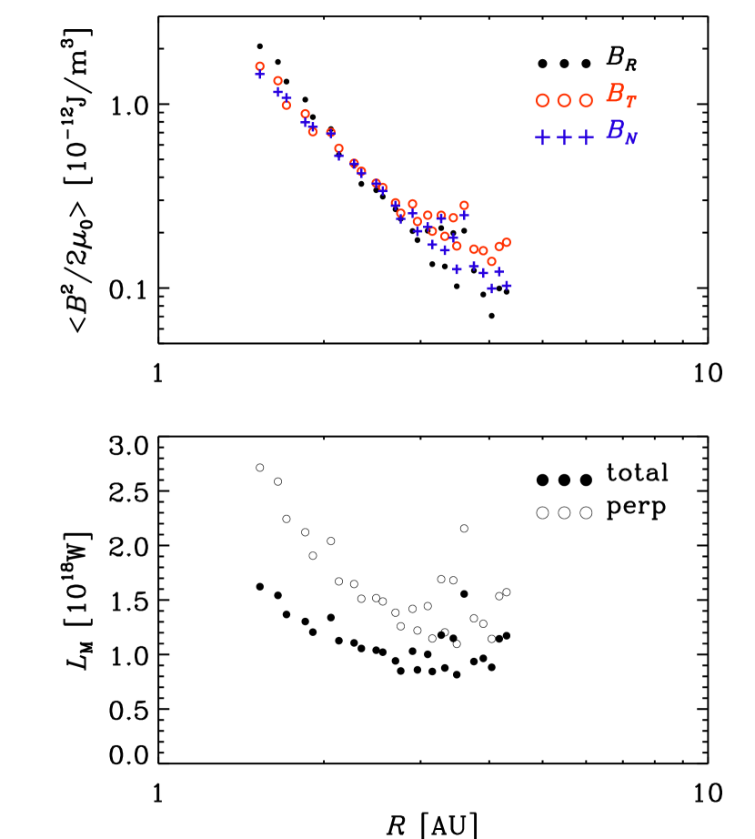
Figure 1.— Magnetic energy density and magnetic luminosity as a function of distance. Note that the decay of magnetic energy is slightly faster than $\propto R^{-2}$ and that the magnetic ‘luminosity’ varies in the range $4$–$8\times 10^{17}\,{\rm W}$.

Next, we focus on the magnetic energy and helicity spectra. We begin by presenting results where we combine data from both hemispheres. As we will verify later, the magnetic helicity has opposite signs in the northern and southern hemispheres, so we multiply the helicity measured in the south by $-1$. Another possibility would be to divide by $\sin\lambda$, but at least for the Parker spiral one does expect a much sharper sign change near the equator than what is expected from a $\sin\lambda$ profile (Bieber et al., 1987a). Furthermore, we distinguish between data sets where the distance to the Sun is either inside or outside $2.8\,{\rm AU}$. In Figure 2 we plot, separately for two separate distance intervals, $2\mu_{0}E_{\rm M}(k)$ and $k|H_{\rm M}(k)|$, rescaled by $4\pi R^{2}$, as well as the relative magnetic helicity, $kH_{\rm M}(k)/2\mu_{0}E_{\rm M}(k)$. We also show a cumulative average of this ratio, starting from the low wavenumber end. This shows quite clearly that the magnetic helicity in the north is negative at small wavenumbers (large length scales) and that it becomes positive at large wavenumbers (small length scales). The cumulative nature of the average slightly overemphasizes the negative contributions, delaying thus the position where the sign changes. The negative magnetic helicity at large scales agrees with that belonging to the Parker spiral, while the positive magnetic helicity at small scales could be the result of turbulent diffusion leading to a reverse transfer of magnetic helicity from large to small scales, as explained in the introduction.

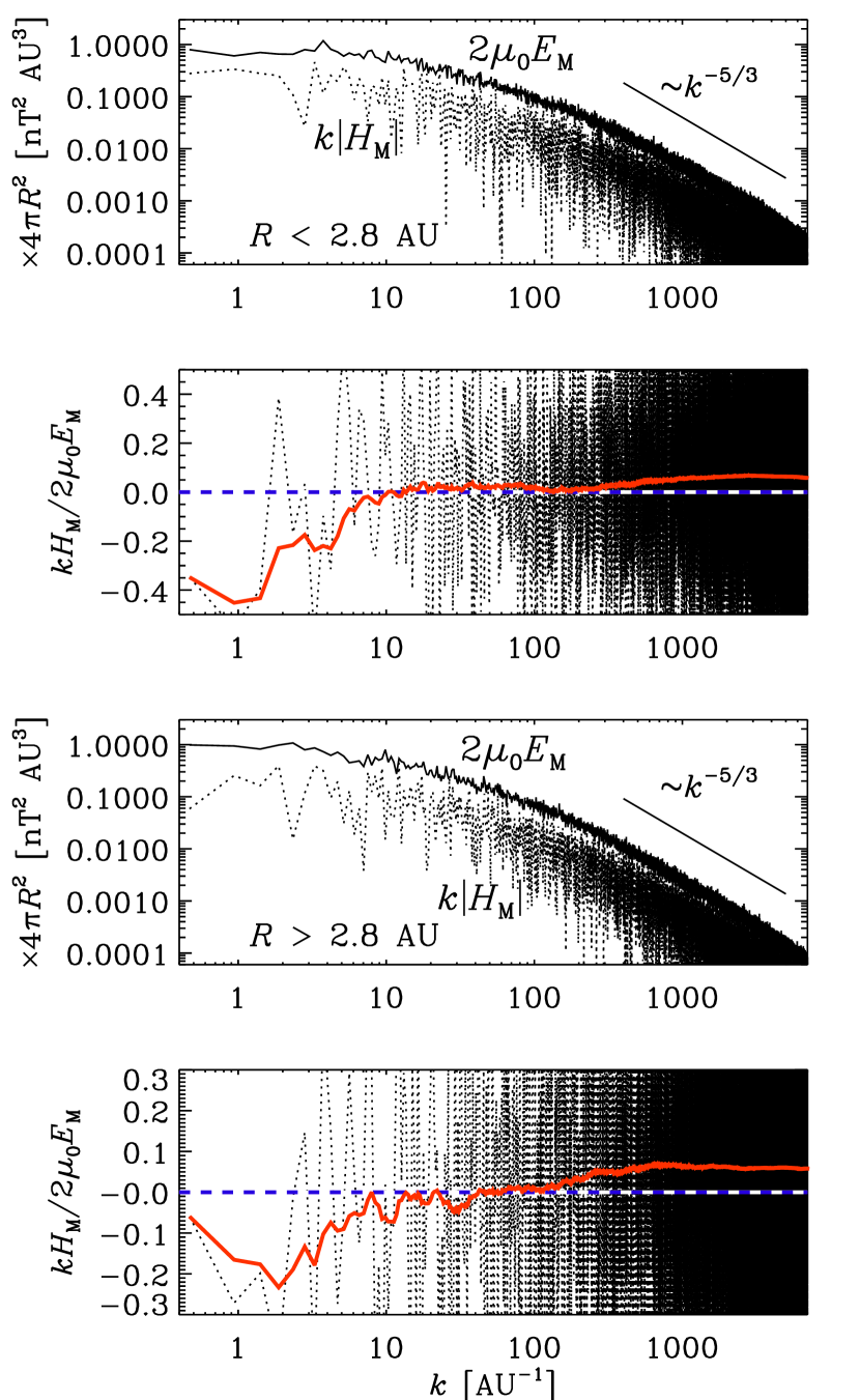
Figure 2.— Magnetic energy and helicity spectra, $2\mu_{0}E_{\rm M}(k)$ and $k|H_{\rm M}(k)|$, respectively, for two separate distance intervals (first and third panels). Furthermore, both spectra are scaled by $4\pi R^{2}$ before averaging within each distance interval above and below $2.8\,{\rm AU}$, respectively. The relative magnetic helicity, $kH_{\rm M}(k)/2\mu_{0}E_{\rm M}(k)$, is plotted separately (second and fourth panels) together with its cumulative average starting from the low wavenumber end. The zero line is shown in dashed.

In the remainder of this paper we use logarithmically spaced wavenumber bins. This way we can reduce the data to a small number of bins and thereby minimize the statistical noise in a more meaningful way. This is shown in Figure 3. In each bin we average the actual values (not the logarithms) of spectral energy and magnetic helicity, both weighted with a $k$ factor. We use rather broad bins, for example the first wavenumber bin at $k=1.5\,{\rm AU}^{-1}$ has a width of $\Delta k=1.2\,{\rm AU}^{-1}$, and the second bin at $k=5.8\,{\rm AU}^{-1}$ has $\Delta k=4.8\,{\rm AU}^{-1}$. Given a maximum length of 1 month for each of the 27 data sets, we have in principle a spectral resolution of $\Delta\Omega=0.2{\rm d}{}^{-1}$, corresponding to $\Delta k=0.5\,{\rm AU}^{-1}$. We use data that were already averaged over $60\,{\rm s}$ time intervals. This corresponds to a spatial resolution of $50\,{\rm Mm}$ and hence a Nyquist wavenumber of $10^{4}\,{\rm AU}^{-1}$. At distances below $2.8\,{\rm AU}$, the magnetic helicity is negative only in the smallest wavenumber bin ($k\approx 1\,{\rm AU}^{-1}$), while at distances beyond $2.8\,{\rm AU}$ the first 3 wavenumber bins ($k<30\,{\rm AU}^{-1}$) show negative helicity.

An estimate for the error has been obtained by comparing with the averages that result by taking only data from the northern or the southern hemisphere into account. The larger one of the two departures is taken as an estimate of the error. This results in a relative uncertainty of our average values by a factor of 1–2.

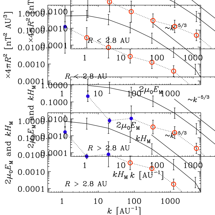
Figure 3.— Magnetic energy and helicity spectra, $2\mu_{0}E_{\rm M}(k)$ and $kH_{\rm M}(k)$, respectively, for two separate distance intervals. Furthermore, both spectra are scaled by $4\pi R^{2}$ before averaging within each distance interval above and below $2.8\,{\rm AU}$, respectively. Filled and open symbols denote negative and positive values of $H_{\rm M}(k)$, respectively.

As explained above, three-dimensional spectra of magnetic energy and magnetic helicity can be obtained by differentiation with respect to $\ln k$. It turns out that, within expected error margins, the three-dimensional spectra are surprisingly close to the one-dimensional spectra. This is shown in Figure 4 where we compare the types of spectra. In view of the fact that the three-dimensional spectra do not seem to alter our conclusions, and since differentiation increases the noise in the data, we restrict ourselves in the following to the discussion of one-dimensional spectra.

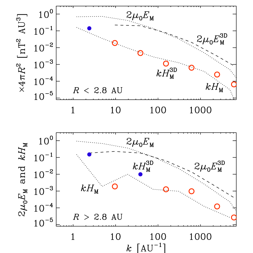
Figure 4.— Comparison between 3D and 1D spectra of magnetic energy and helicity. In both panels the 1D spectra are denoted by dotted lines, while the 3D spectra of magnetic energy by dashed and the 3D spectra of magnetic helicity are indicated by filled and open symbols for negative and positive contributions.

It is worthwhile noting the large separation between both graphs in the ordinate. In other words, $k|H_{\rm M}(k)|\ll 2\mu_{0}E_{\rm M}(k)$. This indicates that the relative magnetic helicity is rather small, which may not be too surprising considering the fact that we have averaged a noisy magnetic helicity result over rather broad wavenumber bins. Also, of course, there is no reason to expect the relative magnetic helicity at the solar surface to be particularly strong. Next, from the open and filled symbols we can see the sign of $H_{\rm M}(k)$, which turns out to be negative at the largest scales (filled symbols) and positive at small scales (open symbols). At a larger distance from the Sun, the break point where the sign of the magnetic helicity changes grows to larger wavenumbers, corresponding to smaller scales. This is probably again related to the effect of turbulent diffusion causing the reversed transfer of magnetic helicity from larger to progressively smaller scales. It could also be a consequence of the growing dominance of the large-scale field (having negative helicity) with distance, so that it would appear as if the magnetic helicity of the large-scale field imprints itself onto the smaller scales. A similar effect has been seen in helical dynamo simulations with an imposed magnetic field (see Fig. 3 of Brandenburg & Matthaeus, 2004), where for sufficiently strong fields the sign of the magnetic helicity is equal to that of the kinetic helicity at small scales. At the same time, the relative magnetic helicity diminishes, which is indeed also seen in Figure 3.

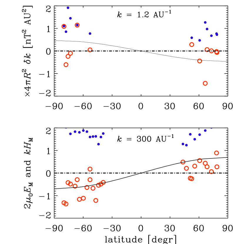
Figure 5.— Magnetic helicity (open symbols) and energy (filled symbols) vs. latitude for data from wavenumber bin $k=1.2\,{\rm AU}^{-1}$ and distances $R<2.8\,{\rm AU}$ (upper panel) and wavenumber bin $k=300\,{\rm AU}^{-1}$ and all distances (lower panel). In the last panel the energy is downscaled by factor 10, because otherwise those data points would lie outside the plot range. The solid lines represent fits proportional to $\sin\lambda$, while dash-dotted lines represent the zero value.

In view of dynamo theory and for comparison with earlier work, it is of interest to compute magnetic helicity fluxes separately for large and small length scales, and integrate them over half the solid angle and over the 11 year cycle, $T_{\rm cyc}$, i.e., we compute

$${\textstyle{1\over 2}}{\cal L}_{\rm H}^{\pm}T_{\rm cyc}=2\pi R^{2}u_{R}T_{\rm cyc}\int_{k\stackrel{{\scriptstyle<}}{{>}}k_{\rm f}}H_{\rm M}(k)\,{\rm d}{}k,$$ (15)

where the 1/2 factor takes the fact into account that one normally gives magnetic helicity fluxes integrated separately for each hemisphere (Berger & Ruzmaikin, 2000). In Table LABEL:Tsummary we give the results for ${\textstyle{1\over 2}}{\cal L}_{\rm H}^{\pm}T_{\rm cyc}$ separately for large ($-$) and small ($+$) scales and also for small and large distances. It turns out that these values are typically around $10^{45}\,{\rm Mx}^{2}/{\rm cycle}$, which is remarkably close to early estimates of Bieber & Rust (1995) of $2\times 10^{45}\,{\rm Mx}^{2}/{\rm cycle}$, and about 10 times below the expected upper limit (Brandenburg, 2009).

Table 1 Results for ${\textstyle{1\over 2}}{\cal L}_{\rm H}^{\pm}T_{\rm cyc}$ in units of $\,{\rm Mx}^{2}/{\rm cycle}$.

Distance  Large Scales  Small Scales $R<2.8\,{\rm AU}$ $-0.9\times 10^{45}$ $+0.3\times 10^{45}$ $R>2.8\,{\rm AU}$ $-1.3\times 10^{45}$ $+0.03\times 10^{45}$

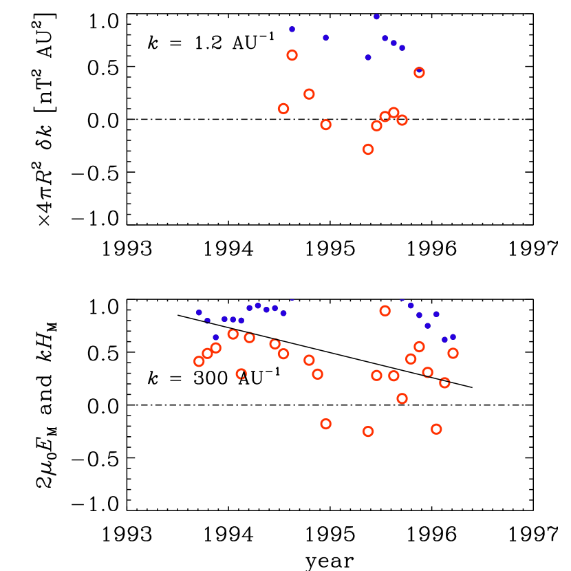
Figure 6.— Similar to Figure 5, but vs. time. Again, in the last panel the energy is downscaled by factor 10, because otherwise those data points would lie outside the plot range. The dash-dotted lines represent the zero value.

Next, we consider the latitudinal dependence by abandoning the averaging over heliographic latitude and consider data from two separate wavenumber bands around 1.2 and $300\,{\rm AU}^{-1}$. The data are obviously very noisy now, especially at low wavenumbers where the wavenumber bins involve fewer data points; see Figure 5. Nevertheless, there is still some evidence for the magnetic helicity having opposite signs in the two hemispheres and, in addition, opposite sign at large ($5\,{\rm AU}$) and small ($0.02\,{\rm AU}\approx 3000\,{\rm Mm}$) length scales ($=2\pi/k$).

The present data have all been taken from the time just after solar maximum and before the next solar minimum. It would therefore be interesting to compare this with measurements taken at other times. There is in principle the possibility that the magnetic helicity could change and even reverse sign for brief time intervals. To see whether already the present data suggest a possible systematic temporal trend, we plot the spectral magnetic helicity in the same two wavenumber bins (around 1.2 and $300\,{\rm AU}^{-1}$) vs. time; see Figure 6. Given the high noise level, it is not possible to conclude anything definite from the plot. Only at large wavenumbers (shown here for $k=300\,{\rm AU}^{-1}$) there might be a meaningful downward trend. Of course, one can only be really sure about this when comparing data over a much longer time span, in which case one might expect to see an oscillatory variation as is also seen in Figures 3 and 4 of Berger & Ruzmaikin (2000).

4. Conclusions

The present results have revealed for the first time evidence that the magnetic helicity in the solar wind has opposite signs at large and small length scales. However, the signs are actually the other way around than what was naively predicted based on the expected signs at the solar surface (Blackman & Brandenburg, 2003), but they do agree with more recent simulations of Brandenburg et al. (2009) and Warnecke et al. (2011a, b) that show a reversed sign some distance away from the dynamo regime due to the effect of turbulent diffusion (without $\alpha$ effect) that tends to forward-cascade magnetic helicity from large to small scales.

Although the solar wind would carry some imprint of the fields generated within the Sun, this field would be deformed due to the fact that the material leaves the Sun with a net angular momentum, and is perhaps turbulent. The magnetic helicity generation by turbulence may be understood using the magnetic helicity conservation equation for the gauge invariant small-scale helicity $h_{\rm f}$ derived by Subramanian & Brandenburg (2006). We have already used this argument in this paper when we associated the effect of turbulent magnetic diffusion with a forward turbulent cascade. Suppose that the wind is turbulent on small scales, then the helicity generation on those scales is governed by $\partial h_{\rm f}/\partial t=-2\overline{\mbox{\boldmath${\cal E}$}}{}\cdot\overline{\mbox{\boldmath$B$}}{}+...$, where $\overline{\mbox{\boldmath${\cal E}$}}{}$ is the mean turbulent electromotive force and the dots refer to microscopic dissipation and possible flux terms. As in mean-field dynamo theory (see, e.g., Brandenburg & Subramanian, 2005), we approximate $\overline{\mbox{\boldmath${\cal E}$}}{}\sim\alpha\overline{\mbox{\boldmath$B$}}{}-\eta_{\rm t}\overline{\mbox{\boldmath$J$}}{}$, where $\overline{\mbox{\boldmath$J$}}{}=\mbox{\boldmath$\nabla$}{}\times\overline{\mbox{\boldmath$B$}}{}$ is the mean current density, and $\alpha$ and $\eta_{\rm t}$ refer to a possible $\alpha$ effect and turbulent diffusion associated with solar wind turbulence, then $\partial h_{\rm f}/\partial t=-2\alpha\overline{\mbox{\boldmath$B$}}{}^{2}+2\eta_{\rm t}\overline{\mbox{\boldmath$B$}}{}\cdot\overline{\mbox{\boldmath$J$}}{}$. The dynamo generated large-scale field $\overline{\mbox{\boldmath$B$}}{}$, which has positive helicity, will then lead through the $\eta_{\rm t}$ term above to small-scale helical fields also with positive $h_{\rm f}$. Moreover, because total helicity is conserved, the turbulent diffusion will put a negative helicity $h_{\rm m}$ on larger scales. Since this $h_{\rm m}$ was originally positive, this leads to a decrease of $h_{\rm m}$. This process may be behind the apparent forward cascade of helicity.

Now consider the large-scale field in the solar wind. Realistically, this field will also have reversals associated with the poloidal field from the Sun reversing every 11 years. However, a unique sense (sign) of its helicity can be imprinted because the sense of rotation of the Sun is always the same, and, in addition, the radial velocity is always outward. We know from the work of Bieber et al. (1987a, b) that this sense is to give negative helicity in the north, opposite to what the dynamo generated mean field had in the solar interior and at the surface. Perhaps the differential rotation in the solar wind pumps negative helicity to the north and positive to the south so as to reverse the original sign of the mean field helicity. One can then explain our current observations as follows: First, the positive helicity seen at larger $k$ is that generated from the turbulent diffusion spreading the helicity of the dynamo-generated mean field to larger $k$ and then advecting this outwards. Second, the Parker spiral eventually leads to a negative helicity on the largest scales (Bieber et al., 1987a). In this picture, the helicity of the Parker field would correspond to scales around $5\,{\rm AU}$ (corresponding to $k=1.2\,{\rm AU}^{-1}$ at $R<2.8\,{\rm AU}$; see Figure 3). This is also in agreement with early work of Smith & Bieber (1993) who found negative magnetic helicity in the north below frequencies of about $10\,\mu{\rm Hz}$, corresponding to $k<20\,{\rm AU}^{-1}$ at a wind speed of about $400\,{\rm km/s}$. However, this scenario needs to be much better explored through simulations such as those of Warnecke et al. (2011b).

Unfortunately, the relative magnetic helicity is rather weak. Therefore, only through extensive averaging we are able to extract any useful information. This low level of relative magnetic helicity suggests that there is efficient mixing taking place in the solar wind, but it could also mean that the magnetic helicity is already rather low at the solar surface. Another possible reason could be the proximity to the solar minimum in 1996.

Although magnetic helicity fluxes are expected to keep their preferred sign over the solar cycle, some modulation is definitely to be expected, as was already found by Smith & Bieber (1993) using measurements spanning the years 1965 to 1988. The data span analyzed in the present work is too short to make any meaningful statements, but one can see that at least at larger wavenumbers there seems to be a decline in magnetic helicity as one progresses further toward solar minimum in 1996.

The present data can be used to extract quantitative estimates for magnetic helicity fluxes. This quantity is normally quoted in Maxwell squared per solar cycle. Assuming that the magnetic helicity during 1993–1996 is representative of the rest of the solar cycle, our analysis suggests values around $10^{45}\,{\rm Mx}^{2}/{\rm cycle}$, which is comparable to the earlier work of Bieber et al. (1987b).

Although the results presented in this paper are physically appealing, there remains uncertainty about the assumptions made in this work, most notably the Taylor hypothesis, which may be problematic over large length scales, but it is expected to be reasonably well satisfied for fluctuations in the inertial range of the turbulent spectrum (see, e.g., Matthaeus & Goldstein, 1982). The assumption of isotropy is only needed when computing three-dimensional spectra. Only the two components in the plane perpendicular to the radial direction enter in our analysis of magnetic helicity. The finite pitch angle of the Parker spiral introduces anisotropy in that plane (Matthaeus et al., 1996). This becomes important at progressively smaller length scales (Wicks et al., 2011), even though the variance of the three components remains similar (see Figure 1). Using spectra of the different components of the magnetic field, Bieber et al. (1996) was able to determine that $\sim 85\%$ of the magnetic energy resides in the perpendicular field fluctuations, while for Ulysses, Smith (2003) found that this value is closer to $50\%$. In any case, it would be useful to estimate magnetic helicity using synthetic data from a numerical simulation. Such an exercise is likely to provide useful insight into the reliability of the assumptions made and the accuracy of the method.

Appendix A Derivation of Equations (10) and (11)

We begin with Eq. (7), but instead of performing the integration over $k_{T}$ and $k_{N}$ we use cylindrical coordinates $(k_{\perp},\phi_{k})$ in Fourier space and assume axisymmetry, so therefore ${\rm d}{}k_{T}{\rm d}{}k_{N}=2\pi k_{\perp}{\rm d}{}k_{\perp}$. Thus, we have

$$M_{ij}^{\rm 1D}(k_{R})=\int_{0}^{2\pi}\int_{0}^{\infty}M_{ij}^{\rm 3D}(k_{R},k_{\perp},\phi_{k})\,k_{\perp}{\rm d}{}k_{\perp}{\rm d}{}\phi_{k}=2\pi\int_{0}^{\infty}M_{ij}^{\rm 3D}(k_{R},k_{\perp})\,k_{\perp}{\rm d}{}k_{\perp}.$$ (A1)

Next, we insert Eq. (3), take the trace, use $k^{2}=k_{R}^{2}+k_{\perp}^{2}$, and substitute $k_{\perp}{\rm d}{}k_{\perp}=k\,{\rm d}{}k$ valid for a fixed $k_{R}$, to carry out the integration over $k$ in the allowed range from $k_{R}$ to $\infty$, and obtain, using Eq. (8),

$$\delta_{ij}M_{ij}^{\rm 1D}(k_{R})=2\pi\int_{k_{R}}^{\infty}2\,{2\mu_{0}E_{\rm M}^{\rm 3D}(k)\over 8\pi k^{2}}\,k\,{\rm d}{}k=\int_{k_{R}}^{\infty}{\mu_{0}E_{\rm M}^{\rm 3D}(k)\over k}\,{\rm d}{}k=\int_{k_{R}}^{\infty}\mu_{0}E_{\rm M}^{\rm 3D}(k)\,{\rm d}{}\ln k,$$ (A2)

which corresponds to Eq. (10). Likewise, multiplying instead with $-2\epsilon_{ijR}{\rm i}k_{R}^{-1}$, and using Eq. (9), we arrive at

$$2\epsilon_{ijR}({\rm i}k_{R})^{-1}M_{ij}^{\rm 1D}(k_{R})=2\pi\int_{k_{R}}^{\infty}4\,{H_{\rm M}^{\rm 3D}(k)\over 8\pi k^{2}}\,k\,{\rm d}{}k=\int_{k_{R}}^{\infty}{H_{\rm M}^{\rm 3D}(k)\over k}\,{\rm d}{}k=\int_{k_{R}}^{\infty}H_{\rm M}^{\rm 3D}(k)\,{\rm d}{}\ln k,$$ (A3)

which corresponds to Eq. (11). In particular, this yields $\mu_{0}E_{\rm M}^{\rm 1D}(k_{R})=|\hat{\mbox{\boldmath$B$}{}}|^{2}$ and $H_{\rm M}^{\rm 1D}(k_{R})=4\,{\rm Im}(\hat{B}_{T}\hat{B}_{N}^{\star})/k_{R}$, as stated just below Eq. (2).

References

- Balogh et al. (1992) Balogh, A., Beek, T. J., Forsyth, R. J., Hedgecock, P. C., Marquedant, R. J., Smith, E. J., Southwood, D. J., & Tsurutani, B. T. 1992, A&AS, 92, 221
- Bao et al. (1999) Bao, S. D., Zhang, H. Q., Ai, G. X., & Zhang, M. 1999, A&AS, 139, 311
- Berger (1997) Berger, M. A. 1997, J. Geophys. Res., 102, 2637
- Berger & Ruzmaikin (2000) Berger, M. A., & Ruzmaikin, A. 2000, J. Geophys. Res., 105, 10481
- Bieber et al. (1987a) Bieber, J. W., Evenson, P. A., & Matthaeus, W. H. 1987a, ApJ, 315, 700
- Bieber et al. (1987b) Bieber, J. W., Evenson, P. A., Matthaeus, W. H. 1987b, J. Geophys. Res., 14, 864
- Bieber & Rust (1995) Bieber, J. W. & Rust, D. M. 1995, ApJ, 453, 911
- Bieber et al. (1996) Bieber, J. W., Wanner, W., & Matthaeus, W. H. 1996, J. Geophys. Res., 101, 2511
- Blackman & Brandenburg (2003) Blackman, E. G., & Brandenburg, A. 2003, ApJ, 584, L99
- Blackman & Field (2000) Blackman, E. G., & Field, G. B. 2000, MNRAS, 318, 724
- Brandenburg (2001) Brandenburg, A. 2001, ApJ, 550, 824
- Brandenburg (2009) Brandenburg, A. 2009, Plasma Phys. Control. Fusion, 51, 124043
- Brandenburg et al. (2009) Brandenburg, A., Candelaresi, S., & Chatterjee, P. 2009, MNRAS, 398, 1414
- Brandenburg & Matthaeus (2004) Brandenburg, A., & Matthaeus, W. H. 2004, Phys. Rev. E, 69, 056407
- Brandenburg & Sandin (2004) Brandenburg, A., & Sandin, C. 2004, A&A, 427, 13
- Brandenburg & Subramanian (2005) Brandenburg, A., & Subramanian, K. 2005, Phys. Rep., 417, 1
- Brandenburg et al. (2003) Brandenburg, A., Blackman, E. G., & Sarson, G. R. 2003, Adv. Space Sci., 32, 1835
- Chae (2000) Chae, J. 2000, ApJ, 540, L115
- Choudhuri et al. (2004) Choudhuri, A. R., Chatterjee, P., & Nandy, D. 2004, ApJ, 615, L57
- Démoulin & Berger (2003) Démoulin, P., & Berger, M. A. 2003, Solar Phys., 215, 203
- Démoulin et al. (2002) Démoulin, P., Mandrini, C. H., van Driel-Gesztelyi, L., Thompson, B. J., Plunkett, S., Kovári, Z., Aulanier, G., & Young, A. 2002, ApJ, 382, 650
- Dikpati & Gilman (2001) Dikpati, M., & Gilman, P. A. 2001, ApJ, 559, 428
- Dobler et al. (2003) Dobler, W., Haugen, N. E. L., Yousef, T. A., & Brandenburg, A. 2003, Phys. Rev. E, 68, 026304
- Freeman (1998) Freeman, J. W. 1998, Geophys. Res. Lett., 15, 88
- Goldstein et al. (1991) Goldstein, M. L., Roberts, D. A., & Fitch, C. A. 1991, Geophys. Res. Lett., 18, 1505
- Goldstein et al. (1995) Goldstein, M. L., Roberts, D. A., & Matthaeus, W. H. 1995, ARA&A, 33, 283
- Ji (1999) Ji, H. 1999, Phys. Rev. Lett., 83, 3198
- Keinigs (1983) Keinigs, R. K. 1983, Phys. Fluids, 26, 2558
- Kleeorin et al. (2000) Kleeorin, N., Moss, D., Rogachevskii, I., & Sokoloff, D. 2000, A&A, 361, L5
- Kusano et al. (2002) Kusano, K., Maeshiro, T., Yokoyama, T., & Sakurai, T. 2002, ApJ, 577, 501
- Matthaeus et al. (1996) Matthaeus, W. H., Ghosh, S., Oughton, S., Roberts, D. A. 1996, J. Geophys. Res., 101, 7619
- Matthaeus & Goldstein (1982) Matthaeus, W. H., & Goldstein 1982, J. Geophys. Res., 87, 6011
- Matthaeus et al. (1986b) Matthaeus, W. H., Goldstein, M. L. & King, J. H. 1986b, J. Geophys. Res., 91, 59
- Matthaeus et al. (1986a) Matthaeus, W. H., Goldstein, M. L. & Lantz, S. R. 1986a, Phys. Fluids, 29, 1504
- Matthaeus et al. (1982) Matthaeus, W. H., Goldstein, M. L., & Smith, C. 1982, Phys. Rev. Lett., 48, 1256
- Moffatt (1969) Moffatt, H. K. 1969, J. Fluid Mech., 35, 117
- Narita et al. (2010) Narita, Y., Sahraoui, F., Goldstein, M. L., & Glassmeier, K. H. 2010, J. Geophys. Res., 115, A04101
- Parker (1958) Parker, E. N. 1958, ApJ, 128, 664
- Pevtsov et al. (1995) Pevtsov, A. A., Canfield, R. C., & Metcalf, T. R. 1995, ApJ, 440, L109
- Pevtsov & Latushko (2000) Pevtsov, A. A. & Latushko, S. M. 2000, ApJ, 528, 999
- Rust & Kumar (1994) Rust, D. M. & Kumar, A. 1994, Solar Phys., 155, 69
- Rust & Kumar (1996) Rust, D. M. & Kumar, A. 1996, ApJ, 464, L199
- Sahraoui et al. (2010) Sahraoui, F., Goldstein, M. L., Belmont, G., Canu, P., & Rezeau, L. 2010, Phys. Rev. Lett., 105, 131101
- Sahraoui et al. (2009) Sahraoui, F., Goldstein, M. L., Robert, P., & Khotyaintsev, Y. V. 2009, Phys. Rev. Lett., 102, 231102
- Seehafer (1990) Seehafer, N. 1990, Solar Phys., 125, 219
- Seehafer (1996) Seehafer, N. 1996, Phys. Rev. E, 53, 1283
- Smith (2003) Smith, C. W. 2003, in AIP Conf. Proc. 679, Proc. Tenth International Solar Wind Conference, ed. M. Velli, R. Bruno, F. Malara, & B. Bucci (Melville, NY: AIP), 413
- Smith & Bieber (1993) Smith, C. W., & Bieber, J. W. 1993, in 23rd International Cosmic Ray Conference, Vol. 3, ed. D. A. Leahy, R. B. Hicks, and D. Venkatesan (Singapore: World Scientific), 493
- Stribling et al. (1995) Stribling T., Matthaeus W. H., & Oughton S. 1995, Phys. Plasmas, 2, 1437
- Subramanian & Brandenburg (2006) Subramanian, K., & Brandenburg, A. 2006, ApJ, 648, L71
- Tu & Marsch (2003) Tu, C.-Y., & Marsch, E. 1995, Spa. Sci. Rev., 73, 1
- Smith et al. (2001) Smith, C. W., Matthaeus, W. H., Zank, G. P., Ness, N. F., Oughton, S., & Richardson, J. D. 2001, J. Geophys. Res., 106, 8253
- Tennekes & Lumley (1972) Tennekes, H., & Lumley, J. L. 1972, First Course in Turbulence (Cambridge: MIT Press)
- Warnecke et al. (2011a) Warnecke, J., Brandenburg, A., & Mitra, D. 2011a, in Advances in Plasma Astrophysics, ed. A. Bonanno et al. (IAU Symp. 274), arXiv:1011.4299
- Warnecke et al. (2011b) Warnecke, J., Brandenburg, A., & Mitra, D. 2011b, A&A, submitted, arxiv:1104.1613
- Webb et al. (2010) Webb, G. M., Hu, Q., Dasgupta, B., & Zank, G. P. 2010, J. Geophys. Res., 115, A10112
- Wicks et al. (2011) Wicks, R. T., Horbury, T. S., Chen, C. H. K., & Schekochihin, A. A. 2011, Phys. Rev. Lett., 106, 045001
- Yousef & Brandenburg (2003) Yousef, T. A., & Brandenburg, A. 2003, A&A, 407, 7
- Zhang et al. (2006) Zhang, H., Sokoloff, D., Rogachevskii, I., Moss, D., Lamburt, V., Kuzanyan, K., & Kleeorin, N. 2006, MNRAS, 365, 276