Simulation of continuous variable quantum games without entanglement

Abstract

A simulation scheme of quantum version of Cournot’s Duopoly is proposed, in which there is a new Nash equilibrium that may be also Pareto optimal without any entanglement involved. The unique property of this simulation scheme is decoherence-free against the symmetric photon loss. Furthermore, we analyze the effects of the asymmetric information on this simulation scheme and investigate the case of asymmetric game caused by asymmetric photon loss. A second-order phase transition-like behavior of the average profits of the firm 1 and firm 2 in Nash equilibrium can be observed with the change of the degree of asymmetry of the information or the degree of ”virtual cooperation”. It is also found that asymmetric photon loss in this simulation scheme plays a similar role with the asymmetric entangled states in the quantum game.

PACS numbers: 02.50.Le, 03.67.-a

I. INTRODUCTION

Recently, significant interests have been focused on generalizing the classical notion of game theory to an analogous quantum version meyer ; eisert , the so-called quantum game theory, which is a new born branch of quantum information theory. Quantum games and quantum strategies can exploit both quantum superposition meyer ; Enk and quantum entanglement eisert ; Enk2002 . Meyer has pointed the way for generalizing the classical game theory to quantum domain by utilizing the quantum superposition meyer , though it has been argued that the Meyer’s scheme can be classically realized Enk . By making use of the entanglement resource, the Prisoner’s Dilemma has been quantized through the scheme of Eisert et al. and shown that the game ceases to pose a dilemma if a restricted quantum strategies are allowed for eisert ; Benjamin2001prl ; Flitney2007pla , which has been experimentally demonstrated by Du et al. Du2002 . Since then more work has been done on quantum prisoners’ dilemma Benjamin2001 ; Iqbal ; Iqbal2004 ; Cao and a number of other games have been generalized to the quantum realm (For review, see Refs.Iqbal2005 ; Guo2008 and references therein). Besides those games in which the players have finite number of strategies, the quantization of classical Cournot’s duopoly in which the players can access to a continuous set of classical strategies has been also investigated Li2002 ; Du2003 ; Li2006 ; Lo2003 ; Lo2005 ; Du2005 ; Zhou ; Qin . Classical Cournot’s duopoly exhibits a dilemma-like situation, in which the unique Nash equilibrium is inferior to the Pareto optimum. For the quantum version of Cournot’s duopoly, even though two players both act as ”selfishly” in the quantum game, they are found to virtually cooperate due to the quantum entanglement between them Li2002 . However, entanglement is usually very fragile against the decoherence caused by the interaction with the surrounding environment. The advantage of most of the previous quantum games are not robust against the noise Johnson2001 and the unique properties of various quantum games different from their classical counterpart will disappear in the limit of decoherence Flitney2005 ; Imoto . However, Chen et al. have discussed decoherence in quantum prisoners’ dilemma Chen2003 , and found some kinds of decoherence have no effects on the Nash equilibria in the quantized prisoners’ dilemma with maximally entangled states. Here, we present the simulation schemes of the quantized symmetric or asymmetric Cournot’s Duopoly, in which there is not any entanglement involved. However, the players can also escape the dilemma-like situation. In this scheme, classical measuring apparatus provides more profits than the quantum measuring apparatus. In the asymmetric game, ”virtual cooperation” does not give any advantage to the weaker of two firms if the degree of the asymmetry exceeds certain threshold value. The most significant aspect of this scheme is its symmetric decoherence-free, namely certain kind of symmetric decoherence does not alter the unique property of this quantized Cournot’s duopoly.

II. CONTINUOUS VARIABLE QUANTUM GAME WITHOUT ENTANGLEMENT

To make this paper self-contained, we briefly outline the classical Cournot’s duopoly and its quantization version in Ref.Li2002 . In a simple version of Cournot’s model for the duopoly, two firms simultaneously decide the quantities $q_{1}$ and $q_{2}$ respectively of a homogeneous product released on the market. Suppose $Q$ is the total quantity, i.e., $Q=q_{1}+q_{2}$, and the market-clearing price is given by $P(Q)=a-Q$ for $Q\leq{a}$ and $P(Q)=0$ for $Q>{a}$. The unit cost of producing the product is assumed to be $c$ with $c<a$. The payoffs or profits of the firms can be written as

$$u_{i}(q_{1},q_{2})=q_{i}[P(Q)-c]=q_{i}[k-(q_{1}+q_{2})],$$ (1)

where $k=a-c$ is a constant and $i=1,2$. Solving for the Nash equilibrium (immune to unilateral deviations) yields the cournot equilibrium,

$$q^{\ast}_{1}=q^{\ast}_{2}=\frac{k}{3}.$$ (2)

At this equilibrium the payoff for the firm $i$ ($i=1,2$) is $k^{2}/9$, which is not the optimal solution. If two firms can cooperate and restrict their quantities to $q^{\prime}_{1}=q^{\prime}_{2}=k/4$, they can both get higher payoff $k^{2}/8$, which is the highest profits they can attain in this symmetric game. However, in a competing game, the objective of each firm is to maximize its individual payoff, and avoid the unilateral deviation causing decrease of its profit. This individual rationality confines the strategies of two firms in the Nash equilibrium point.

The quantization version of the classical Cournot’s duopoly showed that quantum entanglement creates virtual cooperation of two firms and the larger entanglement can guarantee the players (in the Nash equilibrium) a payoff closer to the highest feasible payoff, i.e. the Pareto-optimal payoff. Notwithstanding the domination role of entanglement in various quantum strategies, we attempt to present a simulation scheme of quantized Cournot’s Duopoly, in which there is not any intermediate quantum entanglement involved. We utilize two single-mode optical fields which are initially in the vacuum state $|0\rangle_{1}\otimes|0\rangle_{2}$. Then, two optical fields are sent to firm 1 and firm 2, respectively. The strategic moves of firm 1 and firm 2 are represented by the displacement operators $\hat{D}_{1}$ and $\hat{D}_{2}$ locally acted on their individual optical fields. The players are restricted to choose their strategies from the sets

$$S_{i}=\{\hat{D}_{i}(x_{i})=\exp[\frac{\sqrt{2}}{2}x_{i}(a^{\dagger}_{i}-a_{i})]|x_{i}\in[0,\infty)\},~{}i=1,2$$ (3)

where $a_{i}$ and $a^{\dagger}_{i}$ are the annihilation and creation operators of the $i$th mode optical field, respectively. In this stage, the state of the game becomes a direct product of two coherent states $|\frac{\sqrt{2}}{2}x_{1}\rangle$ and $|\frac{\sqrt{2}}{2}x_{2}\rangle$,

$$|\psi\rangle=|\frac{\sqrt{2}}{2}x_{1}\rangle\otimes|\frac{\sqrt{2}}{2}x_{2}\rangle.$$ (4)

Having executed their moves, firm 1 and firm 2 forward their optical fields to the final measurement, prior to which a beam splitter operation $\hat{J}(\gamma)=\exp[i\gamma({a}^{\dagger}_{1}a_{2}+{a}^{\dagger}_{2}a_{1})]$ ($\gamma\in[0,\frac{\pi}{4})$) is carried out. Therefore the final state prior to the measurement can be expressed as

$$|\Psi\rangle = |\frac{\sqrt{2}}{2}{x}_{1}\cos\gamma+\frac{\sqrt{2}}{2}i{x}_{2}\sin\gamma\rangle$$ (5)

$$\otimes|\frac{\sqrt{2}}{2}{x}_{2}\cos\gamma+\frac{\sqrt{2}}{2}i{x}_{1}\sin\gamma\rangle.$$

Then, a measurement on the photon number of the optical fields is carried out, which is usually done by photon-detector. The measurement is also one of the key issues in quantum games. Different kinds of measurement schemes can alter the characteristics of the games Measurement ; Monty2001 . The measurement schemes mainly depend on the measuring apparatus used. In what follows, we analyze two kinds of measuring apparatuses and investigate their influence on this simulation scheme: (1) ”classical” measuring apparatus which can only give out the expected values of the photon numbers of the optical fields such as the optical power meter. (2) quantum measuring apparatus, such as the highly sensitive quantum photon-counter which can measure the photon number and its distribution.

A. ’Classical’ measuring apparatus

Firstly, we assume only the expected values of the photon number of the optical fields are measured by the ’classical’ measuring apparatus, and the expected values of the photon number are $n_{i}$ ($i=1,2$), which are regarded as the individual quantities. Hence the payoffs are given by

$$u^{Q}_{i}(\hat{D}_{1},\hat{D}_{2})=u_{i}(n_{1},n_{2}),$$ (6)

where the superscript ”Q” denotes ”quantum”. The classical Cournot’s Duopoly can be faithfully represented when $\hat{J}(\gamma)|_{\gamma=0}=I$ (the identity operator), in which the quantities of firm 1 and firm 2 is $n_{1}=x^{2}_{1}/2$ and $n_{2}=x^{2}_{2}/2$, respectively. For the final state in Eq.(5), the measurement gives the respective quantities of two firms

$$n_{1}=\frac{1}{2}(x^{2}_{1}\cos^{2}\gamma+x^{2}_{2}\sin^{2}\gamma),$$

$$n_{2}=\frac{1}{2}(x^{2}_{2}\cos^{2}\gamma+x^{2}_{1}\sin^{2}\gamma).$$ (7)

Then, the quantum profits for two firms are given by

$$u^{Q}_{1}(\hat{D}_{1},\hat{D}_{2})=\frac{1}{2}(x^{2}_{1}\cos^{2}\gamma+x^{2}_{2}\sin^{2}\gamma)[k-\frac{1}{2}(x^{2}_{1}+x^{2}_{2})],$$

$$u^{Q}_{2}(\hat{D}_{1},\hat{D}_{2})=\frac{1}{2}(x^{2}_{2}\cos^{2}\gamma+x^{2}_{1}\sin^{2}\gamma)[k-\frac{1}{2}(x^{2}_{1}+x^{2}_{2})].$$ (8)

Solving for the Nash equilibrium gives the unique one

$$x^{\ast}_{1}=x^{\ast}_{2}=\sqrt{\frac{2k\cos^{2}\gamma}{1+2\cos^{2}\gamma}}.$$ (9)

The profits of two firms at this equilibrium are given by

$$u^{Q}_{1}=u^{Q}_{2}=\frac{k^{2}\cos^{2}\gamma}{(1+2\cos^{2}\gamma)^{2}}.$$ (10)

From Eq.(10), we can see that the profit at the equilibrium increases from the classical payoff $\frac{k^{2}}{9}$ to pareto-optimal payoff $\frac{k^{2}}{8}$ when $\gamma$ increases in the range of $\gamma\in[0,\frac{\pi}{4})$. Obviously, not any intermediate quantum entanglement has been involved in this scheme. But this fact does not impede the successful escaping from the dilemma when $\gamma\rightarrow\frac{\pi}{4}$. It is true that complete classical system can be used to implement the proposed scheme. For example, by making use of the source of classical light or electromagnetic wave, two modulators, beam splitter, and power meters, one can realize this simulation scheme. Though there exists the intermediate entanglement in the quantization scheme of Ref.Li2002 , the final state in Eq.(11) in Ref.Li2002 is also not entangled. In this sense, the present scheme and the one in Ref.Li2002 can be regarded as the same kind but with different definitions of quantum strategies.

B. Quantum measuring apparatus

In this subsection, we assume that a quantum measuring apparatus can be used to measure the photon number distributions of the optical fields. The measured value of photon number is regarded as the quantity of the respective strategy, then the average payoff is calculated based on the probability distribution of the photon number. For the final state in Eq.(5), the payoffs are given by

$$u^{Q}_{i}(\hat{D}_{1},\hat{D}_{2})=\langle{u_{i}(m_{1},m_{2})}\rangle,$$ (11)

where

$$\langle{u_{i}(m_{1},m_{2})}\rangle=\sum^{\infty}_{m_{1},m_{2}=0}u_{i}(m_{1},m_{2})P_{m_{1},m_{2}}$$ (12)

denotes the average of $u_{i}(m_{1},m_{2})$ taken over all possible values of $m_{1}$ and $m_{2}$ with the Poisson distribution

$$P_{m_{1},m_{2}} = e^{-\frac{1}{2}(x^{2}_{1}+x^{2}_{2})}\frac{(\frac{1}{2}(x^{2}_{1}\cos^{2}\gamma+x^{2}_{2}\sin^{2}\gamma))^{m_{1}}}{m_{1}!}$$ (13)

$$\frac{(\frac{1}{2}(x^{2}_{2}\cos^{2}\gamma+x^{2}_{1}\sin^{2}\gamma))^{m_{2}}}{m_{2}!}.$$

For simplicity, we assume $a$ and $c$ tend to infinity but keeping $k=a-c\geq 1$ a finite constant. In this case, the quantum payoffs for two firms are given by

$$u^{Q}_{1}(\hat{D}_{1},\hat{D}_{2})=\frac{1}{2}(x^{2}_{1}\cos^{2}\gamma+x^{2}_{2}\sin^{2}\gamma)[k-1-\frac{1}{2}(x^{2}_{1}+x^{2}_{2})],$$

$$u^{Q}_{2}(\hat{D}_{1},\hat{D}_{2})=\frac{1}{2}(x^{2}_{2}\cos^{2}\gamma+x^{2}_{1}\sin^{2}\gamma)[k-1-\frac{1}{2}(x^{2}_{1}+x^{2}_{2})].$$

In this case, when $\hat{J}(\gamma)=I$ (the identity operator), the scheme can not return to the classical Cournot’s Duopoly. Comparing the payoffs in Eq.(14) and Eq.(8), we can find that quantum fluctuation causes the reduce of the payoffs. Solving for the Nash equilibrium yields the unique one

$$x^{\ast}_{1}=x^{\ast}_{2}=\sqrt{\frac{2(k-1)\cos^{2}\gamma}{1+2\cos^{2}\gamma}}.$$ (15)

The profits of two firms at this equilibrium are given by

$$u^{Q}_{1}=u^{Q}_{2}=\frac{(k-1)^{2}\cos^{2}\gamma}{(1+2\cos^{2}\gamma)^{2}}.$$ (16)

From Eq.(16), we can see that the profit at the equilibrium increases from the $\frac{(k-1)^{2}}{9}$ to $\frac{(k-1)^{2}}{8}$ when $\gamma$ increases from $0$ to $\frac{\pi}{4}$. The above results show the scheme using classical measuring apparatus has advantage to the scheme using the quantum measuring apparatus.

Here, for avoiding the emergence of the situation $m_{1}+m_{2}>a$ with nonzero probability, after Eq.(13) it has been assumed $a$ and $c$ tend to infinite but keeping $k=a-c$ a finite constant, which guarantees the payoff summed over $m_{1}$, $m_{2}$ from $0$ to infinity in Eq.(12) has the analytical expression in Eq.(14). For very large but finite value of $a$ and $c$, the probability $P_{m_{1},m_{2}}$ in Eq.(13) corresponding to $m_{1}+m_{2}>a$ tends to very very small, and the summation of those terms with $m_{1}+m_{2}>a$ in Eq.(12) should be written as the summation of $-cm_{1}P_{m_{1},m_{2}}$ or $-cm_{2}P_{m_{1},m_{2}}$ which also tends to small enough to guarantee the payoff well approximated by the Eq.(14). However, for other cases with small values of $a$, the situation becomes very complicate. The payoff in Eq.(14) is not valid and need to be revised. It is very difficult to obtain an analytical result in this situation. Our numerical results show the optimal payoff of two firms is between $k^{2}/8$ and $(k-1)^{2}/8$ as $\gamma$ tends to $\pi/4$. For examples, in the case with $a=6$, $c=1$, $k=5$, $\gamma=\pi/4$, the optimal payoff is about $2.02487$, which is near $(k-1)^{2}/8=2$; in the case with $a=10$, $c=5$, $k=5$, $\gamma=\pi/4$, the optimal payoff is about $2.00006$. Thus it is conjectured that the conclusion that scheme using classical measuring apparatus has advantage to the scheme using the quantum measuring apparatus is valid even in the cases with small values of $a$ and $c$.

III. SYMMETRIC DECOHERENCE-FREE ASPECTS OF THIS QUANTIZED SCHEME

The most significant characteristics of our simulation scheme is its symmetric decoherence-free. Previous works have shown that the decoherence could destroy the advantage of quantum game Johnson2001 ; Flitney2005 ; Imoto . In our simulation scheme, the advantage of quantum game is robust against the symmetric photon-loss, where the decoherence caused by the photon loss can be described by the following master equation Phoenix1990 ,

$$\frac{\partial\rho(t)}{\partial{t}}=\sum^{2}_{i=1}\kappa\hat{a}_{i}\rho(t)\hat{a}^{\dagger}_{i}-\frac{\kappa}{2}(\hat{a}^{\dagger}_{i}\hat{a}_{i}\rho(t)+\rho(t)\hat{a}^{\dagger}_{i}\hat{a}_{i}),$$ (17)

where $\kappa$ is the decay rate. $\rho(t)$ represents the whole state of the firm 1 and firm 2. The evolving state can be expressed as,

$$|\frac{\sqrt{2}}{2}x_{1}(t)\rangle_{1}|\frac{\sqrt{2}}{2}x_{2}(t)\rangle_{2}$$ (18)

where $|\frac{\sqrt{2}}{2}x_{i}(t)\rangle_{i}=|\frac{\sqrt{2}}{2}x_{i}e^{-\frac{\kappa}{2}t}\rangle_{i}$ ($i=1,2$). Then forward the evolving state into the beam splitter and we have

$$|\Psi(t)\rangle = |\frac{\sqrt{2}}{2}{x}_{1}e^{-\frac{\kappa}{2}t}\cos\gamma+\frac{\sqrt{2}}{2}i{x}_{2}e^{-\frac{\kappa}{2}t}\sin\gamma\rangle$$ (19)

$$\otimes|\frac{\sqrt{2}}{2}{x}_{2}e^{-\frac{\kappa}{2}t}\cos\gamma+\frac{\sqrt{2}}{2}i{x}_{1}e^{-\frac{\kappa}{2}t}\sin\gamma\rangle.$$

From the above quantum state, we can immediately obtain the following conclusion: If both firms have the complete information about the photon loss, they can adjust their strategies according to the transformation $x_{i}\rightarrow{x}_{i}e^{\frac{\kappa}{2}t}$, which can guarantee the final payoffs are invariant under the influence of the photon loss process.

IV. ASYMMETRIC INFORMATION ASPECTS OF THIS SIMULATION SCHEME

Figure 1: (a) The scaled payoff $U_{2}/k^{2}$ of the firm 2 and (b) the scaled payoff $U_{1}/k^{2}$ of the firm 1 at Nash equilibrium are plotted as the function of $\Delta/k$ for different values of $\gamma$ with $\theta=0.5$. (Solid line) $\gamma=0$; (Dash line) $\gamma=\pi/16$; (Dot line) $\gamma=\pi/8$; (Dash dot line) $\gamma=3\pi/16$; (Dash dot dot line) $\gamma=(\frac{\pi}{4})^{-}$.

Figure 2: (a) The scaled payoff $U_{2}/k^{2}$ of the firm 2 and (b) the scaled payoff $U_{1}/k^{2}$ of the firm 1 at Nash equilibrium are plotted as the function of $\gamma$ for different values of $\Delta/k$ with $\theta=0.5$. (Solid line) $\Delta/k=0$; (Dash line) $\Delta/k=0.5$; (Dot line) $\Delta/k=1$; (Dash dot line) $\Delta/k=1.5$; (Dash dot dot line) $\Delta/k=2^{-}$.

Recently, the quantum game with asymmetric information has been investigated and some novel phenomenons caused by asymmetry of information have been revealed Du2003 . It is very interesting to study how the asymmetric information can alter the aspects of the present simulation scheme of the original quantized game. In the case with asymmetric information, firm 1 does not know what $c_{2}$ (firm 2’s unit cost) is, only knows that $c_{2}=c_{H}$ with probability $\theta$ and $c_{2}=c_{L}$ with probability $1-\theta$ ($c_{H}>c_{L}$). Yet firm 2 knows with certainty the unit cost $c_{2}$ of its product as well as that of firm 1’s ($c_{1}$). So, the Eq.(8) should be replaced by

$$u^{Q}_{1}(\hat{D}_{1},\hat{D}_{2}) = \frac{1}{2}(x^{2}_{1}\cos^{2}\gamma+x^{2}_{2}\sin^{2}\gamma)[a-c_{1}-\frac{1}{2}(x^{2}_{1}+x^{2}_{2})],$$

$$u^{Q}_{2H}(\hat{D}_{1},\hat{D}_{2}) = \frac{1}{2}(x^{2}_{2}\cos^{2}\gamma+x^{2}_{1}\sin^{2}\gamma)[a-c_{H}-\frac{1}{2}(x^{2}_{1}+x^{2}_{2})],$$

$$u^{Q}_{2L}(\hat{D}_{1},\hat{D}_{2}) = \frac{1}{2}(x^{2}_{2}\cos^{2}\gamma+x^{2}_{1}\sin^{2}\gamma)[a-c_{L}-\frac{1}{2}(x^{2}_{1}+x^{2}_{2})].$$

For convenience we denote the strategy by $x_{i}$ when it is $\hat{D}_{i}(x_{i})$. Let $\{x^{\ast}_{1},x^{\ast}_{2H},x^{\ast}_{2L}\}$ be the Bayes-Nash equilibrium. Then $x_{2}=x^{\ast}_{2H(L)}$ is chosen to maximize $u^{Q}_{2H(L)}(x^{\ast}_{1},x_{2})$ and $x_{1}=x^{\ast}_{1}$ is chosen to maximize $\theta{u}^{Q}_{1}(x_{1},x^{\ast}_{2H})+(1-\theta){u}^{Q}_{1}(x_{1},x^{\ast}_{2L})$. Solving the three optimization problem yields the Bayes-Nash equilibrium. For simplicity, we assume that $c_{1}=\theta{c_{H}}+(1-\theta)c_{L}$, $k=a-c_{1}$, $\Delta=c_{H}-c_{L}$. After calculation, the unique Bayes-Nash equilibrium can be obtained

$$x^{\ast{2}}_{1} = \frac{2k\cos^{2}\gamma}{1+2\cos^{2}\gamma},$$

$$x^{\ast{2}}_{2H} = \frac{2k\cos^{2}\gamma-4\cos^{4}\gamma(a-c_{H})-(1-\theta)\Delta}{1-4\cos^{4}\gamma},$$

$$x^{\ast{2}}_{2L} = \frac{2k\cos^{2}\gamma-4\cos^{4}\gamma(a-c_{L})+\theta\Delta}{1-4\cos^{4}\gamma}.$$ (21)

In the above derivation, it has been assumed that $\max[\frac{2(c_{H}-c_{1})-k}{k-(c_{H}-c_{1})},0]<\cos(2\gamma)$. When $\frac{2(c_{H}-c_{1})-k}{k-(c_{H}-c_{1})}\geq\cos(2\gamma)>0$, the unique Bayes-Nash equilibrium can be obtained

$$x^{\ast{2}}_{1} = \frac{2\cos^{2}(\gamma)[\theta{k}-\theta(1-\theta)\Delta+k\cos(2\gamma)]}{\theta+\cos(2\gamma)[2+\cos(2\gamma)]},$$

$$x^{\ast{2}}_{2H} = 0,$$

$$x^{\ast{2}}_{2L} = \frac{2\cos^{2}(\gamma)[\theta\Delta+(k+\theta\Delta)\cos(2\gamma)]}{\theta+\cos(2\gamma)[2+\cos(2\gamma)]}.$$ (22)

In the following, we consider the iterative game. When $\frac{2(c_{H}-c_{1})-k}{k-(c_{H}-c_{1})}\geq\cos(2\gamma)>0$, the average profits in the iterative game are given by

$$\bar{U}^{Q}_{1} = [\cos^{2}\gamma(4\theta((k+\Delta(\theta-1))\theta+k\cos 2\gamma)$$

$$\cdot(-2\Delta\theta^{2}+2k\theta+2\Delta\theta+k-2(k(\theta-3)$$

$$+\Delta(\theta-1)\theta)\cos 2\gamma+k\cos 4\gamma)\cos^{2}\gamma$$

$$+(\theta-1)(2(k(\theta-2)+\Delta\theta(\theta+1))\cos 2\gamma$$

$$+\theta(-2k+\Delta+2\Delta\theta+\Delta\cos 4\gamma))$$

$$\cdot(2(\Delta(\theta-1)\theta+k(\theta+2))\cos 2\gamma$$

$$+\theta(2k-\Delta+2\Delta\theta-\Delta\cos 4\gamma)))]$$

$$/[4(2\theta+4\cos 2\gamma+\cos 4\gamma+1)^{2}]$$

$$\bar{U}^{Q}_{2} = [\cos^{2}\gamma(4\theta((k+\Delta(\theta-1))\theta+k\cos 2\gamma)$$ (23)

$$\cdot(2\Delta\theta^{2}+2k\theta+k-2\Delta-2(k(\theta-3)$$

$$+\Delta(\theta^{2}-5\theta+4))\cos 2\gamma$$

$$+(k+2\Delta(\theta-1))\cos 4\gamma)\sin^{2}\gamma$$

$$-(\theta-1)(\theta(2k+\Delta+2\Delta\theta+\Delta\cos 4\gamma)$$

$$-2(k(\theta-2)+\Delta(\theta-3)\theta)\cos 2\gamma)^{2})]$$

$$/[4(2\theta+4\cos 2\gamma+\cos 4\gamma+1)^{2}].$$

When $\max[\frac{2(c_{H}-c_{1})-k}{k-(c_{H}-c_{1})},0]<\cos(2\gamma)$, the average profits in the iterative game are given by

$$\bar{U}^{Q}_{1} = \frac{4[k^{2}-\Delta^{2}\theta(1-\theta)]}{8(2+\cos 2\gamma)^{2}}$$

$$+\frac{[4k^{2}+\Delta^{2}\theta(1-\theta)\cos 2\gamma(3+\cos 2\gamma)]\cos 2\gamma}{8(2+\cos 2\gamma)^{2}},$$

$$\bar{U}^{Q}_{2} = \bar{U}^{Q}_{1}+\frac{1}{4}\Delta^{2}\theta(1-\theta).$$ (24)

From the above results, one can find a boundary which separates two parameter regions A and B labeled by the inequality $\max[\frac{2(c_{H}-c_{1})-k}{k-(c_{H}-c_{1})},0]<\cos(2\gamma)$ and $\max[\frac{2(c_{H}-c_{1})-k}{k-(c_{H}-c_{1})},0]\geq\cos(2\gamma)$, respectively. In the parameter region A, the profits in Nash-equilibrium in Eq.(24) return to the ones of Ref.Du2003 if replacing $\cos 2\gamma$ by $\exp[-2\gamma]$ in Ref.Du2003 . While in the parameter region B, due to the constraint that the strategy in Bayes-Nash equilibrium should not exceed the strategy space $[0,\infty)$. we give out the profits of Bayes-Nash equilibrium in Eq.(23) which is different with the results in Ref.Du2003 .

In Fig.1, the rescaled average profits of the firm 1 and 2 are plotted as the function of $\Delta/k$ for different values of $\gamma$. For a fixed value of $\theta$, the degree of asymmetry $\xi\equiv\frac{\Delta^{2}(1-\theta)\theta}{k^{2}}$ is monotonic with $\Delta/k$. The profit of the firm 2 increases with the degree of asymmetry, and the profit of the firm 1 decreases with the degree of asymmetry except for the case with $\gamma=0$, $\theta=0.5$ and $\Delta/k<\frac{4}{3}$, in which the rescaled profit $\bar{U}^{Q}_{1}/k^{2}$ of the firm 1 keeps fixed. When $\gamma<\frac{\pi}{4}$, a second-order phase transition-like behaviors (i.e. $\frac{\partial{\bar{U}^{Q}_{i}}/k^{2}}{\partial{\Delta/k}}$ ($i=1,2$) is discontinuous) of the rescaled average profits of the firm 1 and firm 2 in Bayes-Nash equilibrium may be observed as the degree of asymmetry varies across the boundary of the parameter regions A and B. In Fig.2, the rescaled average profits of the firm 1 and 2 are plotted as the function of $\gamma$ for different values of $\Delta/k$. The asymmetric property of this game can significantly affect the dependence of the average profits of both firm 1 and 2 on the degree of ”virtual cooperation” $\sin(2\gamma)$. For $\theta=1/2$ and $0<\Delta/k<\frac{4\sqrt{3}}{9}$, both the profits of the firm 1 and 2 firstly increase with $\gamma$ and then decrease with $\gamma$. While for larger asymmetry with $\theta=1/2$ and $2>\Delta/k>\frac{4\sqrt{3}}{9}$, both the profits of the firm 1 and 2 decrease with $\gamma$. The above results imply that, in this case, the ”virtual cooperation” has advantage role only in the nearly symmetric or very small asymmetric games. If the degree of asymmetry exceeds a threshold, the ”virtual cooperation” in this game can suppress the gain of the firm standing on the advantage side with more information. But for the firm standing on the disadvantage side due to less information, the ”virtual cooperation” should be regarded as one disaster after another. Similarly, when $\theta=1/2$ and $\Delta/k>1$, a second-order phase transition-like behaviors (i.e. $\frac{\partial{\bar{U}^{Q}_{i}/k^{2}}}{\partial{\gamma}}$ ($i=1,2$) is discontinuous) of the rescaled average profits of the firm 1 and firm 2 in Nash equilibrium can be observed as the parameter $\gamma$ varies across the boundary of the parameter regions A and B. In Fig.3, we calculate the total rescaled profit of firm 1 and 2 versus the parameters $\Delta/k$ or $\gamma$ for $\theta=1/2$. It is found that in the ”ideal virtual cooperation” case with $\gamma={\frac{\pi}{4}}^{-}$, the total profit in Nash equilibrium is invariant against the asymmetry of this game. In other cases, the total profit always increases with $\Delta/k$. The smaller the parameter $\gamma$, the more significant influence of the asymmetry on the total profit.

Figure 3: (a) The scaled total payoff $(U_{1}+U_{2})/k^{2}$ at Nash equilibrium of two firms is plotted as the function of $\gamma$ for different values of $\Delta/k$ with $\theta=0.5$. (Solid line) $\Delta/k=0$; (Dash line) $\Delta/k=0.5$; (Dot line) $\Delta/k=1$; (Dash dot line) $\Delta/k=1.5$; (Dash dot dot line) $\Delta/k=2^{-}$. (b) The scaled total payoff $(U_{1}+U_{2})/k^{2}$ at Nash equilibrium of two firms is plotted as the function of $\Delta/k$ for different values of $\gamma$ with $\theta=0.5$. (Solid line) $\gamma=0$; (Dash line) $\gamma=\pi/16$; (Dot line) $\gamma=\pi/8$; (Dash dot line) $\gamma=3\pi/16$; (Dash dot dot line) $\gamma=(\frac{\pi}{4})^{-}$.

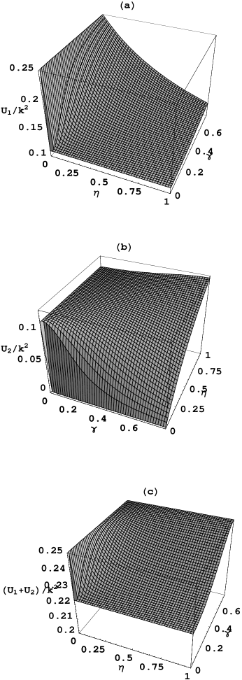
Figure 4: (a) The scaled payoff $U_{1}/k^{2}$ of the firm 1, (b) the scaled payoff $U_{2}/k^{2}$ of the firm 2, and (c) the scaled total payoff $(U_{1}+U_{2})/k^{2}$ at Nash equilibrium are plotted as the functions of $\gamma$ and $\eta$.

V. DECOHERENCE-INDUCED ASYMMETRIC QUANTUM GAME

In the Ref.Li2006 , by making use of the asymmetrical entangled states, the quantum model shows some kind of ”encouraging” and ”suppressing” effect in profit functions of different players. Here we discuss how the asymmetric decoherence can alter the Bayes-Nash equilibrium of the above quantized scheme of the Cournot’s Duopoly, where the asymmetric decoherence means that two firms experience two different degrees of decoherence. Let us consider the following specific case in which the firm 2 encounters a decoherence caused by the photon loss with the loss rate $\sqrt{\eta}=e^{-\kappa{\tau}/2}$ ($\tau\in[0,\infty)$) just before the final photon counting. Obviously, the final measurement gives the respective quantities of the two firms

$$n_{1}=\frac{1}{2}(x^{2}_{1}\cos^{2}\gamma+x^{2}_{2}\sin^{2}\gamma),$$

$$n_{2}=\frac{\eta}{2}(x^{2}_{2}\cos^{2}\gamma+x^{2}_{1}\sin^{2}\gamma).$$ (25)

Substituting the Eq.(25) into the payoff function, and solving the two optimization problems yields the Bayes-Nash equilibrium. For $0<\eta\leq 1$ and $0\leq\gamma\leq\frac{\pi}{4}$, the unique Bayes-Nash equilibrium can be obtained

$$x^{\ast{2}}_{1}=\frac{8k\eta\cos^{2}\gamma}{1+\eta(6+\eta)+4\eta\cos 2\gamma-(1-\eta)^{2}\cos 4\gamma},$$

$$x^{\ast{2}}_{2}=\frac{8k\cos^{2}\gamma}{1+\eta(6+\eta)+4\eta\cos 2\gamma-(1-\eta)^{2}\cos 4\gamma}.$$ (26)

Meanwhile, the corresponding profits at the Bayes-Nash equilibrium can be obtained

$${U}^{Q}_{1}=\xi[1+\eta-(1-\eta)\cos 2\gamma],$$

$${U}^{Q}_{2}=\xi\eta[1+\eta+(1-\eta)\cos 2\gamma],$$ (27)

where

$$\xi=\frac{2k^{2}\cos^{2}\gamma[(1+\eta)^{2}-(1-\eta)^{2}\cos^{2}2\gamma]}{[1+\eta(6+\eta)+4\eta\cos 2\gamma-(1-\eta)^{2}\cos 4\gamma]^{2}}$$ (28)

When $\eta\rightarrow 0$, ${U}^{Q}_{1}\rightarrow\frac{k^{2}}{4+5\delta_{\gamma,0}}$ and ${U}^{Q}_{2}\rightarrow\frac{k^{2}\delta_{\gamma,0}}{9}$, where $\delta_{\gamma,0}$ equals 1 for $\gamma=0$ and is zero elsewhere. When $\gamma=0$, ${U}^{Q}_{1}={U}^{Q}_{2}=\frac{k^{2}}{9}$, which shows the payoff does not depend on $\eta$ and implies the Nash equilibrium of the classical game is robust against the asymmetric photon-loss.

In Fig.4, the rescaled profits of two firms in the Nash equilibrium are plotted as the function of $\gamma$ and $\eta$. For $\gamma\neq 0$, the asymmetric decoherence encourages the profit ${U}^{Q}_{1}$ of the firm 1 and suppresses the profit ${U}^{Q}_{2}$ of the firm 2. We can find ${U}^{Q}_{1}$ and ${U}^{Q}_{2}$ exhibit the sharp decline and ascent in the end of asymmetric photon loss for those cases with very small value of $\gamma\neq 0$. In the initial stage of photon-loss with $\eta>0.5$, ”virtual cooperation” accelerates the encouragement and suppression effects of the asymmetric photon loss. The asymmetric photon loss plays a role in transferring the profit from the firm 2 to firm 1. Surprisingly, the asymmetric photon loss can improve the total profits of the firm 1 and 2 in the Nash equilibrium in the situations with $0<\gamma<\frac{\pi}{4}$. In the ideal ”virtual cooperation”, i.e. $\gamma=\frac{\pi}{4}$, the total profits are kept fixed against the asymmetric photon loss.

VI. CONCLUSIONS

In this paper, we present a simulation scheme of the continuous variable quantized Cournot’s duopoly, in which not any intermediate quantum entanglement has been involved. The influence of measuring apparatus, symmetric or asymmetric photon loss, and asymmetric information on their Nash equilibria has been investigated. It is shown that the scheme using classical measuring apparatus is advantage to the one using the quantum measuring apparatus. Being different from the previous quantized Cournot’s duopoly involving entanglement, this simulation scheme is also symmetric photon loss free; While for asymmetric photon loss, the profits in Nash equilibrium exhibit a transfer from one firm to the other. Simultaneously, the total profit in Nash equilibrium increases with the asymmetric photon loss except for two extreme cases, i.e. the complete no ”virtual cooperation” case and the ideal ”virtual cooperation” case.

In the cases with asymmetric information, a second-order phase transition-like behavior of the average profits of the firm 1 and firm 2 in Nash equilibrium can be observed as the degree of asymmetry or the degree of ”virtual cooperation” vary. The ”virtual cooperation” has advantage role for total profit in Nash equilibrium only in the nearly symmetric or very small asymmetric games. If the degree of asymmetry exceeds a threshold value, the ”virtual cooperation” in this game can suppress the gain of the firm standing on the advantage side with more information. But for the firm standing on the disadvantage side due to less information, the ”virtual cooperation” should be regarded as one disaster after another. For the total profit, it is found that, in the ”ideal virtual cooperation” case with $\gamma={\frac{\pi}{4}}^{-}$, the total profit in Nash equilibrium is invariant against the asymmetry of this game. In other cases with $\gamma<\frac{\pi}{4}$, the total profit always increases with $\Delta/k$. The smaller the parameter $\gamma$, the more significant influence of the asymmetry on the total profit.

References

- (1) D. Meyer, Phys. Rev. Lett. 82, 1052 (1999).
- (2) J. Eisert et al., Phys. Rev. Lett. 83, 3077 (1999).
- (3) S.J. van Enk. Phys. Rev. Lett. 84, 789 (2000); D. A. Meyer. Phys. Rev. Lett. 84, 790 (2000).
- (4) S.J. van Enk, R. Pike, Phys. Rev. A 66, 024306 (2002).
- (5) S.C. Benjamin and P.M. Hayden, Phys. Rev. Lett. 87, 069801 (2001).
- (6) A.P. Flitney and L.C.L. Hollenberg, Phys. Lett. A 363, 381 (2007).
- (7) J. Du, H. Li, X. Xu, M. Shi, J. Wu, X. Zhou, and R. Han, Phys. Rev. Lett. 88, 137902 (2002).
- (8) S.C. Benjamin and P.M. Hayden, Phys. Rev. A 64, 030301 (2001).
- (9) A. Iqbal, J. Phys. A: Math. Gen. 37, L353 (2004).
- (10) A. Iqbal, S. Weigert, J. Phys. A: Math. Gen. 37 5873 (2004).
- (11) S. Cao and M.-F. Fang, Chin. Phys. 15, 276 (2006).
- (12) A. Iqbal, Ph.D thesis, Quaid-i-Azam University, Pakistan.
- (13) H. Li, J. Du and S. Massar, Phys. Lett. A 306, 73 (2002).
- (14) J. Du, H. Li, C. Ju, Phys. Rev. E 68, 016124 (2003).
- (15) Y. Li, G. Qin, X. Zhou, J. Du, Phys. Lett. A 355, 447 (2006).
- (16) C.F. Lo, D. Kiang, Phys. Lett. A 318, 333 (2003).
- (17) C.F. Lo, D. Kiang, Phys. Lett. A 346, 65 (2005).
- (18) J. Du, C. Ju, and H. Li, J. Phys. A: Math. Gen. 38, 1559 (2005).
- (19) J. Zhou, L. Ma, Y. Li, Phys. Lett. A 339, 10 (2005).
- (20) G. Qin, X. Chen, M. Sun, X. Zhou, and J. Du, Phys. Lett. A 340, 78, (2005).
- (21) N.F. Johnson, Phys. Rev. A 63, 020302 (2001).
- (22) A.P. Flitney, D. Abbott, J. Phys. A: Math. Gen. 38, 449 (2005).
- (23) S.K. Özdemir, J. Shimamura, and N. Imoto, Phys. Lett. A 325, 104 (2004).
- (24) L.K. Chen, H. Ang, D. Kiang, L.C. Kwek, and C.F. Lo, Phys. Lett. A 316, 317 (2003).
- (25) A. Nawaz, A.H. Toor, J. Phys. A: Math. Gen. 39 2791 (2006).
- (26) C.F. Li, Y.S. Zhang, Y.F. Huang, G.C. Guo, Phys. Lett. A 280, 257 (2001).
- (27) S.J.D. Phoenix, Phys. Rev. Lett. 41, 5132 (1990).
- (28) H. Guo, J. Zhang and G. J. Koehler, Decis. Support Syst. 46, 318 (2008).