SLAC–PUB–14352 January, 2011

Simplifying Multi-Jet QCD Computation

Michael E. Peskin

SLAC, Stanford University
2575 Sand Hill Rd., Menlo Park, CA 94025 USA

ABSTRACT

These lectures give a pedagogical discussion of the computation of QCD tree amplitudes for collider physics. The tools reviewed are spinor products, color ordering, MHV amplitudes, and the Britto-Cachazo-Feng-Witten recursion formula.

PRESENTED AT

Mini-courses of the XIII Mexican School of Particles and Fields

University of Sonora, Hermosillo, Mexico

October 2–5, 2008

and

LHC Physics Summer School

Tsinghua University, Beijing, China

August, 16–20, 2010

1 Introduction

As the LHC begins operation, the number one topic of the day is QCD. To a first approximation, everything that happens at the LHC is determined by QCD. Events from new physics at the LHC will appear, if we are lucky, at fractions of a part per billion of the proton-proton total cross section. They will appear at rates ten thousand times smaller than Drell-Yan processes, and a hundred times smaller than top quark pair production. This requires that we understand those Standard Model processes at a level that includes their dressing with QCD radiation.

Since the 1980’s, there has been considerable work on methods for QCD computation. The primary goal of this work has been to make seemingly impossible calculations doable. In the early 1980’s, it was beyond the state of the art to compute to lowest order the rates at hadron colliders for $W^{+}$ production with three jets. Recently, this process has been computed at the 1-loop level, a computation that, if done by textbook methods, would have required thousands of Feynman diagrams, each one an integral over millions of terms [1, 2].

A byproduct of this improved understanding of QCD computation is that calculations of reasonable difficulty by textbook methods become trivial when approached with the new methods. In the LHC era, every graduate student ought to be able to calculate the QCD amplitudes for multijet processes. In this lecture, I will give you some tools to do that.

I will first review a set of ideas developed in the 1980’s. Sections 2, 3, and 4 will develop, in turn, the ideas of spinor products, color ordering, and MHV amplitudes. In Section 5, I will illustrate how these methods make the somewhat strenuous calculation of the most basic quark and gluon cross sections a triviality. In Section 6, I will review a relatively new wrinkle in this technology, the Britto-Cachazo-Feng-Witten recursion formula. In Section 7, I will apply that formula to compute the Drell-Yan cross sections with one and two jets. I hope that this last example will give a persuasive illustration of the power of these methods.

There are many references for those who would like to learn more. The first three topics are reviewed very beautifully in a 1991 Physics Reports article by Mangano and Parke [3] and in the 1995 TASI lectures by Dixon [4]. The newer set of calculational tools are described in recent review articles by Bern, Dixon, and Kosower [5] and Berger and Forde [6]. These last articles are especially concerned with technology that extends the ideas presented here to the computation of loop amplitudes.

Loop calculations, though, are beyond the scope of these lectures. My only goal here is to do easy calculations. I hope that these lectures will help you extend the domain of QCD calculations to which you will apply this term.

In parallel with learning these methods, it will be useful for you to explore some of the available computer programs that automatically generate matrix elements for multi-particle processes and also carry out Monte Carlo integration over phase space, a topic that is not discussed in these lectures. A particularly accessible and powerful code is MADGRAPH/MADEVENT [7, 8]. An important advanced code is SHERPA [9, 10] with the matrix element generator COMIX [11]. It is always good, though, to know what is inside the black box and to have tools for extending what is available there. For that, I hope these lectures will provide useful background.

2 Spinor products

Perturbative QCD is primarily concerned with the interactions of gluons and quarks at momentum scales for which the masses of these particles can be ignored. It is well-known, and discussed in the textbooks, that massless particles can be labeled by their helicity. For massless states, the helicity is a well-defined, Lorentz-invariant quantity. The basic goal of these lectures will be to compute tree amplitudes for massless quark and gluon states of definite helicity.

In the 1980’s, Berends and Wu spearheaded an effort to compute amplitudes for massless particles by exploiting the property that their lightlike momentum vectors can be decomposed into spinors [12]. Using this idea, scattering amplitudes can be written in terms of Lorentz-invariant contractions of spinors, spinor products.

2.1 Massless fermions

Consider a massless fermion of mommentum $p$. The spinors for this fermion satisfy the Dirac equation

$$\not{\hbox{\kern-2.0pt$p$}}\ U(p)=0$$ (1)

There are two solutions to this equation, the spinors for right- and left-handed fermions. In a basis where the Dirac matrices take the form

$$\gamma^{\mu}=\pmatrix{0&\sigma^{\mu}\cr\overline{\sigma}^{\mu}&0\cr}\ ,\qquad\gamma^{5}=\pmatrix{-1&0\cr 0&1\cr}$$ (2)

where $\sigma^{\mu}=(1,\vec{\sigma})$, $\overline{\sigma}^{\mu}=(1,-\vec{\sigma})$, these spinors take the form

$$U_{R}(p)=\pmatrix{0\cr u_{R}(p)\cr}\ ,\qquad U_{L}(p)=\pmatrix{u_{L}(p)\cr 0\cr}\ ,$$ (3)

where the entries are 2-component spinors satisfying

$$p\cdot\sigma\ u_{R}=0\ ,\qquad p\cdot\overline{\sigma}\ u_{L}=0\ .$$ (4)

Each equation has one unique solution. The spinor $u_{R}(p)$ can be related to the spinor $u_{L}(p)$ by

$$u_{R}(p)=i\sigma^{2}u^{*}_{L}(p)\ ,$$ (5)

since this transformation turns a solution of one of the equations (4) into a solution to the other. This equation also gives a phase convention for $u_{R}(p)$ that I will use throughout these lectures.

To describe antiparticles, we also need solutions $V(p)$ that describe their creation and destruction. However, for massless particles, $V(p)$ satisfies the same equation as $U(p)$. We can then use the same solutions for these quantities, with $u_{R}$ and $u_{L}$ related as above. The spinor $V_{R}(p)$ is used for the creation of a left-handed antifermion; the spinor $V_{L}(p)$ is used for the creation of a right-handed antifermion.

In the discussion to follow, it will be simplest to treat all particles as final states of the amplitudes we are considering. The outgoing left- and right-handed fermions will be represented by the spinors $\overline{U}_{L}$ and $\overline{U}_{R}$ and outgoing left- and right-handed antifermions will be represented by the spinors $U_{R}$ and $U_{L}$. I will recover initial-state particles by crossing, that is, by starting from the amplitude with the antiparticle in the final state and evaluating that amplitude for a 4-momentum with negative time component.

I will represent these spinors compactly as

$$\overline{U}_{L}(p)=\langle p\ ,\quad\overline{U}_{R}(p)=[p\ ,\quad U_{L}(p)=p]\ ,\quad U_{R}(p)=p\rangle\ ,$$ (6)

The Lorentz-invariant spinor products can then be standardized as

$$\overline{U}_{L}(p)U_{R}(q)=\langle pq\rangle\ ,\qquad\overline{U}_{R}(p)U_{L}(q)=[pq]\ .$$ (7)

The quantities on the right-hands sides are called simply angle brackets and square brackets. The spinors are related to their lightlike 4-vectors by the identities

$$p\rangle[p=U_{R}(p)\overline{U}_{R}(p)=\not{\hbox{\kern-2.0pt$p$}}({1-\gamma^{5}\over 2})\ ,\quad p]\langle p=U_{L}(p)\overline{U}_{L}(p)=\not{\hbox{\kern-2.0pt$p$}}({1+\gamma^{5}\over 2})$$ (8)

From these formulae, we can derive some basic properties of the brackets. First,

$$\langle pq\rangle=[qp]^{*}\ .$$ (9)

Next, multiplying two matrices from (8) and taking the trace,

$$\langle pq\rangle[qp]={\mbox{\rm tr}}[\not{\hbox{\kern-2.0pt$q$}}\not{\hbox{\kern-2.0pt$p$}}({1+\gamma^{5}\over 2})]=2p\cdot q$$ (10)

so that

$$|\langle pq\rangle|^{2}=|[qp]|^{2}=2p\cdot q\ .$$ (11)

Finally, using (5),

$$\langle pq\rangle=u^{\dagger}_{L}(p)u_{R}(q)=u^{*}_{La}(p)(i\sigma^{2})_{ab}u^{*}_{Lb}(q)\ .$$ (12)

Then, by the antisymmetry of $\sigma^{2}$,

$$\langle pq\rangle=-\langle qp\rangle\,\qquad[pq]=-[qp]\ .$$ (13)

We now see that the brackets are square roots of the corresponding Lorentz vector products, and that they are antisymmetric in their two arguments.

Some further identities are useful in discussing vector currents built from spinors. First,

$$\overline{U}_{L}(p)\gamma^{\mu}U_{L}(q)=u_{L}^{\dagger}(p)\overline{\sigma}^{\mu}u_{L}(q)\ ,\quad\overline{U}_{R}(p)\gamma^{\mu}U_{R}(q)=u_{R}^{\dagger}(p)\sigma^{\mu}u_{R}(q)\ .$$ (14)

The relationship between $u_{L}(p)$ and $u_{R}(p)$ in (5) implies that we can rearrange

$$u^{\dagger}_{L}(p)\overline{\sigma}^{\mu}u_{L}(q) = u^{\dagger}_{L}(p)\overline{\sigma}^{\mu}(-(i\sigma^{2})^{2})u_{L}(q)$$ (15)

$$= u^{\dagger}_{L}(p)(-i\sigma^{2})\sigma^{\mu T}(i\sigma^{2})u_{L}(q)$$

$$= u_{R}^{T}(p)\sigma^{\mu T}u^{*}_{R}(q)$$

$$= u_{R}^{\dagger}(q)\sigma^{\mu}u_{R}(p)\ ,$$

From this, it follows that

$$\langle p\gamma^{\mu}q]=[q\gamma^{\mu}p\rangle\ .$$ (16)

The Fierz identity, the identity of sigma matrices

$$(\overline{\sigma}^{\mu})_{ab}(\overline{\sigma}_{\mu})_{cd}=2(i\sigma^{2})_{ac}(i\sigma^{2})_{bd}\ ,$$ (17)

allows the simplification of contractions of spinor expressions. In a matter similar to (15), the relation (17) can be used to show

$$\langle p\gamma^{\mu}q]\langle k\gamma_{\mu}\ell]=2\langle pk\rangle[\ell q]\ ,\qquad\langle p\gamma^{\mu}q][k\gamma_{\mu}\ell\rangle=2\langle p\ell\rangle[kq]\ .$$ (18)

Finally, spinor products obey the Schouten identity

$$\langle ij\rangle\langle k\ell\rangle+\langle ik\rangle\langle\ell j\rangle+\langle i\ell\rangle\langle jk\rangle = 0$$

$$[ij][k\ell]+[ik][\ell j]+[i\ell][jk] = 0\ .$$ (19)

To prove this identity, note that the expressions on the left are totally antisymmetric in $j,k,\ell$. But, antisymmetrizing three 2-component objects gives zero.

The identities presented in this section will allow us to reduce complex spinor expressions to functions of angle brackets and square brackets, which are the square roots of the Lorentz products of lightlike vectors. In the following, I will denote these Lorentz products using the notation

$$s_{ij}=2p_{i}\cdot p_{j}=(p_{i}+p_{j})^{2}\ .$$ (20)

To evaluate simple expressions written in terms of spinor products, we can often think of the whole expression as the square root of an expression in terms of the $s_{ij}$. However, for more complex expressions, it is usually easiest to directly evaluate the spinor products from their component momenta. I give formulae for evaluating spinor products in Appendix A.

2.2 $e^{+}e^{-}\to\mu^{+}\mu^{-}$

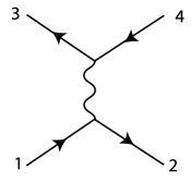
Figure 1: Feynman diagram for $e_{L}^{-}e_{R}^{+}\to\mu^{-}_{L}\mu^{+}_{R}$.

At this point, we are already able to perform some interesting computations. Consider, for example, the tree-level amplitude for $e_{L}^{-}e_{R}^{+}\to\mu^{-}_{L}\mu^{+}_{R}$ in QED. This is given by the diagram shown in Fig. 1. Label the momenta as in the diagram, considering all momenta as outgoing. Then the amplitude is

$$i{\cal M} = (-ie)^{2}\ {-i\over q^{2}}\ \overline{U}_{L}(3)\gamma^{\mu}U_{L}(4)\,\overline{U}_{L}(2)\gamma_{\mu}U_{L}(1)$$ (21)

$$= {ie^{2}\over q^{2}}\langle 3\gamma^{\mu}4]\langle 2\gamma_{\mu}1]$$

$$= {2ie^{2}\over q^{2}}\langle 32\rangle[14]\ ,$$

where I have used (18) in the last step. Now, $\langle 32\rangle$ and $[14]$ are both square roots of

$$s_{23}=(k_{2}+k_{3})^{2}=(k_{1}+k_{4})^{2}$$ (22)

which is just the Mandelstam invariant $u$. In the $e^{+}e^{-}$ center of mass frame, $u=-2E^{2}(1+\cos\theta)$, and $q^{2}=s=4E^{2}$. Then

$$|i{\cal M}|^{2}=e^{4}(1+\cos\theta)^{2}\ .$$ (23)

This is a familiar result, and we have obtained it with surprising ease.

Actually, we can simplify the result further. In the denominator of (21), $q^{2}=2k_{1}\cdot k_{2}=\langle 12\rangle[21]$. Multiply the numerator and denominator of (21) by $\langle 32\rangle$, to give

$$i{\cal M}=2ie^{2}{\langle 32\rangle[14]\langle 32\rangle\over\langle 12\rangle[21]\langle 32\rangle}\ .$$ (24)

Then, in the denominator

$$[21]\langle 32\rangle=[12]\langle 23\rangle=[1\not{\hbox{\kern-2.0pt$2$}}\ 3\rangle=[1(-\not{\hbox{\kern-2.0pt$1$}}-\not{\hbox{\kern-2.0pt$3$}}-\not{\hbox{\kern-2.0pt$4$}})3\rangle$$ (25)

Using the Dirac equation, $\not{\hbox{\kern-2.0pt$1$}}1]=0$, $\not{\hbox{\kern-2.0pt$3$}}3\rangle=0$. This leaves $(-[14]\langle 43\rangle)$. The last square brackets cancel and we find

$$i{\cal M}=2ie^{2}{{\langle 23\rangle}^{2}\over\langle 12\rangle\langle 34\rangle}\ .$$ (26)

The entire expression can be written in terms of angle brackets with no square brackets. Similarly, if we had multiplied instead by

$${[14]\over[14]}$$ (27)

a similar set of manipulations would have given

$$i{\cal M}=2ie^{2}{{[14]}^{2}\over[12][34]}\ ,$$ (28)

with square brackets only.

2.3 Massless photons

This simplification of amplitudes with fermions extends to amplitudes with massless vector bosons. I will show that the polarization vectors for final-state massless vector bosons of definite helicity can be represented as [13, 14, 15]

$$\epsilon^{*\mu}_{R}(k)={1\over\sqrt{2}}{\langle r\gamma^{\mu}k]\over\langle rk\rangle}\ ,\qquad\epsilon^{*\mu}_{L}(k)=-{1\over\sqrt{2}}{[r\gamma^{\mu}k\rangle\over[rk]}\ .$$ (29)

Here $k$ is the momentum of the vector boson and $r$ is some other fixed lightlike 4-vector, called the reference vector. The only requirement on $r$ is that it cannot be collinear with $k$.

Here is the argument: First, note that (29) satisfies the basic properties

$$[\epsilon^{*}_{R}(k)]^{*}=\epsilon_{L}^{*}(k)\,\qquad k_{\mu}\epsilon^{*\mu}_{R,L}(k)=0\ .$$ (30)

The second condition follows from $\not{\hbox{\kern-2.0pt$k$}}\,k]=0$. Also,

$$\epsilon_{R}^{*}(k)\cdot[\epsilon_{L}^{*}(k)]^{*}=\epsilon_{R}^{*}(k)\cdot\epsilon_{R}^{*}(k)=0\ ,$$ (31)

because, by (18), this expression is proportional to $\langle rr\rangle=0$. Finally,

$$|\epsilon_{R}^{*}(k)|^{2}=\frac{1}{2}{\langle r{\gamma^{\mu}}k]\langle k{\gamma_{\mu}}r]\over\langle rk\rangle[kr]}={2\over 2}{\langle rk\rangle[rk]\over\langle rk\rangle[kr]}=-1\ .$$ (32)

Then

$$|\epsilon^{*}_{R}(k)|^{2}=|\epsilon^{*}_{L}(k)|^{2}=-1\ ,\qquad\epsilon^{*}_{R}(k)\cdot[\epsilon^{*}_{L}(k)]^{*}=0\ .$$ (33)

as required for polarization vectors.

Next, evaluate the formulae for the $\epsilon^{*}_{R,L}$ for a particular choice of the reference vector $r$. For $k=(k,0,0,k)$, let $r=(r,0,0,-r)$. The associated spinors are

$$u_{L}(k)=\sqrt{2k}\pmatrix{0\cr 1\cr}\,\quad u_{R}(k)=\sqrt{2k}\pmatrix{1\cr 0\cr}\ ,\quad u_{L}(r)=\sqrt{2r}\pmatrix{-1\cr 0\cr}\ .$$ (34)

Then

$$\langle r{\gamma^{\mu}}k] = u^{\dagger}_{L}(r)\overline{\sigma}^{\mu}u_{L}(k)=\sqrt{4kr}\ (0,1,-i,0)^{\mu}$$

$$\langle rk\rangle = u^{\dagger}_{L}(r)u_{L}(k)=-\sqrt{4kr}$$ (35)

For this choice of $r$, $\epsilon^{*}_{R}(k)$ is manifestly the right-handed polarization vector,

$$\epsilon^{*\mu}_{R}(k)=-{1\over\sqrt{2}}(0,1,i,0)^{*}$$ (36)

Finally, analyze how (29) changes when we change the reference vector $r$ to a different lightlike vector $s$.

$$\epsilon^{*\mu}_{R}(k;r)-\epsilon^{*\mu}_{R}(k;s) = {1\over\sqrt{2}}\left({{\langle r{\gamma^{\mu}}k]}\over\langle rk\rangle}-{{\langle s{\gamma^{\mu}}k]}\over\langle sk\rangle}\right)$$ (37)

$$= {1\over\sqrt{2}}{1\over\langle rk\rangle\langle sk\rangle}(-\langle r{\gamma^{\mu}}k]\langle ks\rangle+{\langle s{\gamma^{\mu}}k]}\langle kr\rangle)$$

$$= {1\over\sqrt{2}}{1\over\langle rk\rangle\langle sk\rangle}(-\langle r{\gamma^{\mu}}\not{\hbox{\kern-2.0pt$k$}}s\rangle+\langle s{\gamma^{\mu}}\not{\hbox{\kern-2.0pt$k$}}r\rangle)$$

$$= {1\over\sqrt{2}}{1\over\langle rk\rangle\langle sk\rangle}\langle s(\not{\hbox{\kern-2.0pt$k$}}\gamma^{\mu}+{\gamma^{\mu}}\not{\hbox{\kern-2.0pt$k$}})r\rangle$$

$$= {1\over\sqrt{2}}{1\over\langle rk\rangle\langle sk\rangle}\cdot 2k^{\mu}\langle sr\rangle\ .$$

The last line follows from the anticommutator of Dirac matrices. The final result of this calculation is that

$$\epsilon^{*\mu}_{R}(k;r)-\epsilon^{*\mu}_{R}(k;s)=f(r,s)k^{\mu}\ .$$ (38)

where $f(r,s)$ is a function of the two reference vectors. This expression, when dotted into an on-shell photon or gluon amplitude, will give zero by the Ward identity, as shown in Fig. 2. Thus—as long as we are computing a gauge-invariant set of Feynman diagrams—we can use any convenient reference vector $s$ and obtain the same answer as we would with the particular reference vector $r$ used in (36).

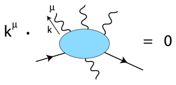
Figure 2: Ward identity obeyed by a gauge-invariant sum of diagrams with all external particles on shell.

This completes the justification of the representation (29) of massless photon or gluon polarization vectors. From here on, because I will in any case consider all momenta as outgoing, I will drop the explicit $*$’s on the polarization vectors.

2.4 $e^{+}e^{-}\to\gamma\gamma$

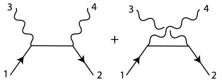
Figure 3: Feynman diagram for $e_{L}^{-}e_{R}^{+}\to\gamma\gamma$.

We can illustrate the application of these polarization vectors by computing the amplitudes for $e_{L}^{-}e_{R}^{+}\to\gamma\gamma$. Label the momenta as in Fig. 3, taking all momenta as outgoing. Then the value of the amplitude for this process is

$$i{\cal M}=(-ie)^{2}\langle 2\left\{\gamma\cdot\epsilon(4){i(2+4)\over s_{24}}\gamma\cdot\epsilon(3)+\gamma\cdot\epsilon(3){i(2+3)\over s_{23}}\gamma\cdot\epsilon(4)\right\}1]\ .$$ (39)

We will choose explicit polarization vectors $\epsilon(3)$, $\epsilon(4)$ to evaluate this amplitude for each choice of photon helicities. This formula also introduces some additional streamlining of the notation: I write $(2+4)$, instead of $(\not{\hbox{\kern-2.0pt$k$}}_{2}+\not{\hbox{\kern-2.0pt$k$}}_{4})$ or even $(\not{\hbox{\kern-2.0pt$2$}}+\not{\hbox{\kern-2.0pt$4$}})$, and I use (20) to express the denominators.

There are four possible choices for the photon polarizations. However the cases $\gamma_{R}\gamma_{L}$ and $\gamma_{L}\gamma_{R}$ are related by interchange of the momenta 3 and 4. The cases $\gamma_{R}\gamma_{R}$ and $\gamma_{L}\gamma_{L}$ are related by parity, which interchanges states with $R$ and $L$ polarization. Further, it is easy to see that the amplitudes for $\gamma_{R}\gamma_{R}$ and $\gamma_{L}\gamma_{L}$ are actually zero. For the case of $\gamma_{R}\gamma_{R}$, choose $r=2$ for both polarization vectors,

$$\epsilon^{\mu}(3)={1\over\sqrt{2}}{\langle 2\gamma^{\mu}3]\over\langle 23\rangle}\ ,\qquad\epsilon^{\mu}(4)={1\over\sqrt{2}}{\langle 2{\gamma^{\mu}}4]\over\langle 24\rangle}\ .$$ (40)

When these choices are used in (39), we find, with the use of the Fierz identity (18)

$$\langle 2\gamma\cdot\epsilon(4)\ \sim\ 2\langle 22\rangle[4\ =\ 0\ ,$$ (41)

which vanishes because $\langle 22\rangle=0$. A similar cancellation occurs with $\epsilon(3)$. So the entire matrix element vanishes. The amplitude for the case $\gamma_{L}\gamma_{L}$ must then also vanish by parity; alternatively, we can find the same cancellation for that case by using $r=1$ in both polarization vectors.

To compute the amplitude for the case $\gamma_{R}\gamma_{L}$, choose

$$\epsilon^{\mu}(3)={1\over\sqrt{2}}{\langle 2\gamma^{\mu}3]\over\langle 23\rangle}\ ,\qquad\epsilon^{\mu}(4)=-{1\over\sqrt{2}}{[1{\gamma^{\mu}}4\rangle\over[14]}\ .$$ (42)

Then the second diagram in Fig. 3 vanishes by the logic of the previous paragraph. Using the Fierz identity, the first diagram gives

$$i{\cal M} = {-ie^{2}\over s_{24}}{2\cdot 2\over(-2)\langle 23\rangle[14]}\langle 24\rangle[1(2+4)2\rangle[31]$$ (43)

$$= {2ie^{2}\over s_{13}\langle 23\rangle[14]}\langle 24\rangle[14]\langle 42\rangle[31]$$

$$= {2ie^{2}\over\langle 13\rangle[31]\langle 23\rangle[14]}\langle 24\rangle[14]\langle 42\rangle[31]$$

$$= 2ie^{2}{(\langle 24\rangle)^{2}\over\langle 23\rangle\langle 31\rangle}$$

In terms of the Mandelstam variables, $s_{23}=u$, $s_{13}=s_{24}=t$, so

$$|i{\cal M}|^{2}=4e^{4}{t\over u}=4e^{4}{1-\cos\theta\over 1+\cos\theta}\ ,$$ (44)

which is the well-known correct answer. In this case, the calculation gave directly the simplified form of the expression that involves only angle brackets and no square brackets.

The methods of this section can be generalized to massive external particles. For the treatment of $W$ and $Z$ bosons, see Section 7. An efficient formalism for the treatment of massive fermions is presented in [16].

3 Color-ordered amplitudes

We could now apply this spinor product technology directly to QCD. However, it will be useful first to spend a bit of effort analyzing the color structure of QCD amplitudes. It is convenient to divide QCD amplitudes into irreducible, gauge-invariant components of definite color structure. We will see that it is most straightforward to compute these objects separately and then recombine them to obtain the full QCD results.

3.1 $q\overline{q}\to gg$

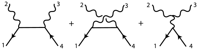
Figure 4: Feynman diagrams for $q_{L}\overline{q}_{R}\to gg$.

Begin with the process $q_{L}\overline{q}_{R}\to gg$. This is similar to the process $e^{+}e^{-}\to\gamma\gamma$ analyzed in the previous section, except that now there are three diagrams, as shown in Fig. 4, including one with a 3-gluon vertex. With the numbering of external states as in the figure and all momenta outgoing, the value of the amplitude is

$$i{\cal M} = (ig)^{2}\langle 1\left\{\gamma\cdot\epsilon(2){i(1+2)\over s_{12}}t^{a}t^{b}\gamma\cdot\epsilon(3)+\gamma\cdot\epsilon(3){i(1+3)\over s_{13}}t^{b}t^{a}\gamma\cdot\epsilon(2)\right\}4]$$ (45)

$$+(ig)(-gf^{abc}t^{c}){-i\over s_{14}}\langle 1{\gamma^{\lambda}}4]\cdot\biggl{(}\epsilon(2)\cdot\epsilon(3)(2-3)_{\lambda}$$

$$\hskip 36.135pt+\epsilon_{\lambda}(3)(2\cdot 3+2)\cdot\epsilon(2)+\epsilon_{\lambda}(2)(-2\cdot 2-3)\cdot\epsilon(3)\biggr{)}\ .$$

In this formula, $t^{a}$ and $t^{b}$ are the color $SU(3)$ representation matrices coupling to the gluons 2 and 3, respectively. The third diagram in Fig. 4 has a color structure that can be brought into the forms seen in the first two diagrams by writing

$$-gf^{abc}t^{c}=(ig)\cdot if^{abc}t^{c}=(ig)(t^{a}t^{b}-t^{b}t^{a})\ .$$ (46)

We will find it convenient to rescale the color matrices: $T^{a}=\sqrt{2}t^{a}$, so that the $T^{a}$ are normalized to

$${\mbox{\rm tr}}[T^{a}T^{b}]=\delta^{ab}\ .$$ (47)

We can then write the amplitude in (45) in the form

$$i{\cal M}=i{\bf M}(1234)\cdot T^{a}T^{b}+i{\bf M}(1324)\cdot T^{b}T^{a}\ ,$$ (48)

with

$$i{\bf M}(1234) = ({ig\over\sqrt{2}})^{2}\biggl{[}\langle 1\gamma\cdot\epsilon(2){i(1+2)\over s_{12}}\gamma\cdot\epsilon(3)4]$$ (49)

$$\hskip 28.45274pt+{-i\over s_{23}}\langle 1\gamma^{\lambda}4][\epsilon(2)\cdot\epsilon(3)(2-3)_{\lambda}$$

$$\hskip 71.13188pt+\epsilon_{\lambda}(3)(2\cdot 3+2)\cdot\epsilon(2)+\epsilon_{\lambda}(2)(-2\cdot 2-3)\cdot\epsilon(3)]\ .$$

In the second term of (48), ${\bf M}(1324)$ is given by the same expression with $(2,\epsilon(2))$ exchanged with $(3,\epsilon(3))$.

The elements $i{\bf M}$ are called color-ordered amplitudes. The complete helicity amplitudes such as (48) are gauge-invariant for any choice of helicities of the external particles and for any Yang-Mills gauge group. The two color factors $T^{a}T^{b}$ and $T^{b}T^{a}$ are independent in any non-Abelian gauge group. Thus, the color-ordered amplitudes must be separately gauge-invariant. This important observation means that we can apply all of the simplifications discussed in the previous section to individual color-ordered amplitudes. It will be much simpler to work with these objects rather than with the full QCD amplitudes.

A consequence of this idea is that the individual color-ordered amplitudes should obey the Ward identity. It is not difficult to verify this for (49). Replace $\epsilon(2)$ by the four-vector 2, and use the properties that the external momenta are lightlike, that $\langle 1$ and $4]$ satisfy the Dirac equation, and that $3\cdot\epsilon(3)=0$. Then all terms in the resulting expression cancel.

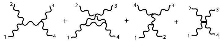
Figure 5: Feynman diagrams for $gg\to gg$.

Other QCD amplitudes can also be reduced to color-ordered structures. Another case that will be important for us is the 4-gluon amplitude shown in Fig. 5. This amplitude can be written in the form

$$i{\cal M} = i{\bf M}(1234)\cdot{\mbox{\rm tr}}[T^{a}T^{b}T^{c}T^{d}]+i{\bf M}(1243)\cdot{\mbox{\rm tr}}[T^{a}T^{b}T^{d}T^{c}]$$ (50)

$$+i{\bf M}(1324)\cdot{\mbox{\rm tr}}[T^{a}T^{c}T^{b}T^{d}]+i{\bf M}(1342)\cdot{\mbox{\rm tr}}[T^{a}T^{c}T^{d}T^{b}]$$

$$+i{\bf M}(1423)\cdot{\mbox{\rm tr}}[T^{a}T^{d}T^{b}T^{c}]+i{\bf M}(1432)\cdot{\mbox{\rm tr}}[T^{a}T^{d}T^{c}T^{b}]\ .$$

I have used the cyclic invariance of the trace to move $T^{a}$ to the front in each trace. Then there are $3!=6$ possible traces, all of which should be included. For a sufficiently large $SU(N)$ gauge group, all of these traces are independent; thus, each coefficient is a gauge-invariant structure. As in the case of $q\overline{q}gg$, these coefficients are given by a single function evaluated with different permutations of the external momenta.

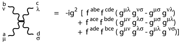
Figure 6: The four gluon vertex of QCD.

To write the four diagrams in Fig. 5 as a sum of color structures, we need to convert color factors in the 3- and 4-gluon vertices into products of $T^{a}$ matrices. For the 3-gluon vertex, this is done through (46), or, by the use of (47), through

$$-gf^{abc}={ig\over\sqrt{2}}{\mbox{\rm tr}}[T^{a}T^{b}T^{c}-T^{a}T^{c}T^{b}]\ .$$ (51)

For the 4-gluon vertex, we need to apply this decomposition twice. The textbook form of the 4-gluon vertex is shown in Fig. 6. Each term can be manipulated as follows

$$-ig^{2}f^{abe}f^{cde} = i{g^{2}\over 2}{\mbox{\rm tr}}([T^{a},T^{b}][T^{c},T^{d}])$$ (52)

$$= i{g^{2}\over 2}{\mbox{\rm tr}}(T^{a}T^{b}T^{c}T^{d}-T^{a}T^{b}T^{d}T^{c}-T^{b}T^{a}T^{c}T^{d}+T^{b}T^{a}T^{d}T^{c})$$

The full 4-gluon vertex can then be rearranged into

$$i{g^{2}\over 2}{\mbox{\rm tr}}(T^{a}T^{b}T^{c}T^{d})[2g^{\mu\lambda}g^{\nu\sigma}-g^{\mu\nu}g^{\lambda\sigma}-g^{\mu\sigma}g^{\nu\lambda}]$$ (53)

plus 5 more terms corresponding to the other 5 color structures in (50).

These vertices in the form of traces over $T^{a}$’s can be contracted using the identity for $SU(N)$ generators

$$T^{a}_{ij}T^{a}_{k\ell}=\delta_{i\ell}\delta_{kj}-{1\over N}\delta_{ij}\delta_{k\ell}\ .$$ (54)

The coefficients in this equation are determined by the normalization (47), with $\delta^{aa}=N^{2}-1$, the number of generators of $SU(N)$, and by the requirement that ${\mbox{\rm tr}}T^{a}=0$. Using this identity, a product of traces can be transformed into a single trace plus smaller factors, for example,

$${\mbox{\rm tr}}[T^{a}A]{\mbox{\rm tr}}[T^{a}B]={\mbox{\rm tr}}AB-{1\over N}{\mbox{\rm tr}}[A]{\mbox{\rm tr}}[B]\ .$$ (55)

Using these methods, the value of a Feynman diagram is naturally organized as a sum of color-ordered terms. The individual color-ordered amplitudes are computed with color-ordered Feynman rules, shown in Fig. 7.

Using these rules applied to the two diagrams in Fig. 8, it is easy to rederive the color-ordered amplitude (49).

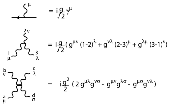
Figure 7: Color-ordered Feynman rules for QCD.

As an example, I will compute the color-ordered amplitude ${\bf M}(1234)$ that is used to build up the four-gluon amplitude. Of the four Feynman diagrams in Fig. 5, only the three diagrams shown in Fig. 9 contribute to this color-ordered component. Here and in the rest of the lectures, the color-ordered amplitudes in the figures will be ordered clockwise. Using the Feynman rules in Fig. 7, we find

$$i{\bf M}(1234) = ({ig\over\sqrt{2}})^{2}\biggl{[}{-i\over s_{14}}[\epsilon(4)\cdot\epsilon(1)(4-1)^{\lambda}+\epsilon^{\lambda}(1)(2\,1+4)\cdot\epsilon(4)+\epsilon^{\lambda}(4)(-2\,4-1)\cdot\epsilon(1)]$$ (56)

$$\hskip 21.68121pt\cdot[\epsilon(2)\cdot\epsilon(3)(2-3)_{\lambda}+\epsilon_{\lambda}(3)(2\,3+2)\cdot\epsilon(2)+\epsilon_{\lambda}(2)(-2\,2-3)\cdot\epsilon(3)]$$

$$+{-i\over s_{12}}[\epsilon(1)\cdot\epsilon(2)(1-2)^{\lambda}+\epsilon^{\lambda}(2)(2\,2+1)\cdot\epsilon(1)+\epsilon^{\lambda}(1)(-2\,1-2)\cdot\epsilon(2)]$$

$$\hskip 21.68121pt\cdot[\epsilon(3)\cdot\epsilon(4)(3-4)_{\lambda}+\epsilon_{\lambda}(4)(2\,4+3)\cdot\epsilon(3)+\epsilon_{\lambda}(3)(-2\,3-4)\cdot\epsilon(2)]$$

$$\hskip-21.68121pt+(-i)[2\epsilon(1)\cdot\epsilon(3)\,\epsilon(2)\cdot\epsilon(4)-\epsilon(1)\cdot\epsilon(2)\,\epsilon(3)\cdot\epsilon(4)-\epsilon(1)\cdot\epsilon(4)\,\epsilon(2)\cdot\epsilon(3)]\biggr{]}\ .$$

With some effort, you can show that this expression obeys the Ward identity. That demonstrates explicitly that this color component is independently gauge-invariant, as required.

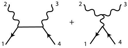
Figure 8: Feynman diagrams contributing to the first color-ordered amplitude in $q\overline{q}\to gg$.

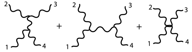
Figure 9: Feynman diagrams contributing to the first color-ordered amplitude in $gg\to gg$.

4 MHV amplitudes

Now that we have reduced the $q\overline{q}gg$ and $gggg$ QCD amplitudes to managable components, it is time to evalute these expressions. We will see that the values we find fall into surprisingly simple forms.

4.1 $q\overline{q}gg$ amplitude

Begin with the $q\overline{q}gg$ amplitude (49). As in the example with $e^{+}e^{-}\gamma\gamma$ in Section 2, we need to consider all possible cases of gluon helicity. From here on, I will notate helicity states by $+$, $-$ instead of $R$, $L$.

Consider first the case $g_{+}g_{+}$. Choose the polarization vectors with reference vector $r=1$,

$$\epsilon^{\mu}(2)={1\over\sqrt{2}}{\langle 1{\gamma^{\mu}}2]\over\langle 12\rangle}\qquad\epsilon^{\mu}(3)={1\over\sqrt{2}}{\langle 1{\gamma^{\mu}}3]\over\langle 13\rangle}\ .$$ (57)

As with (41), the first line of (49) is proportional to $\langle 11\rangle=0$. Also, in the second line of (49), each term contains one of the elements $\epsilon(2)\cdot\epsilon(3)$, $\langle 1\gamma\cdot\epsilon(2)4]$, and $\langle 1\gamma\cdot\epsilon(3)4]$, all of which are proportional to $\langle 11\rangle$. So, the entire expression vanishes. A similar argument shows that the color-ordered amplitude with two negative helicities vanishes.

The two cases with one positive and one negative gluon helicity are distinct color-ordered amplitudes, not related by Bose symmetry. So, both must be computed. I will begin with the case $g_{+}(2)g_{-}(3)$. Choose for the polarization vectors

$$\epsilon^{\mu}(2)={1\over\sqrt{2}}{\langle 1{\gamma^{\mu}}2]\over\langle 12\rangle}\qquad\epsilon^{\mu}(3)=-{1\over\sqrt{2}}{[4{\gamma^{\mu}}3\rangle\over[43]}\ .$$ (58)

Then all terms in ${\bf M}$ vanish except for the term in the second line with $\epsilon(2)\cdot\epsilon(3)$. This factor is

$$\epsilon(2)\cdot\epsilon(3)=-{1\over 2}{2\langle 13\rangle[42]\over\langle 12\rangle[43]}\ .$$ (59)

Then

$$i{\bf M} = {ig^{2}\over 2}{\langle 1\,{(2-3)}\,4]\over\langle 23\rangle[32]}\bigl{(}-{\langle 13\rangle[42]\over\langle 12\rangle[43]}\bigr{)}$$ (60)

$$= -ig^{2}{{\langle 13\rangle}^{2}[42]\over\langle 23\rangle[32]\langle 12\rangle}$$

Again, we can find a simpler form by multiplying top and bottom by $\langle 13\rangle$. Using $\langle 13\rangle[32]=-\langle 14\rangle[42]$, we find

$$i{\bf M}={ig^{2}}{{\langle 13\rangle}^{3}\langle 43\rangle\over\langle 12\rangle\langle 23\rangle\langle 34\rangle\langle 41\rangle}\ .$$ (61)

For the case $g_{-}(2)g_{+}(3)$, choose for the polarization vectors

$$\epsilon^{\mu}(2)=-{1\over\sqrt{2}}{[3{\gamma^{\mu}}2\rangle\over[32]}\qquad\epsilon^{\mu}(3)={1\over\sqrt{2}}{\langle 2{\gamma^{\mu}}3]\over\langle 23\rangle}\ .$$ (62)

For this choice of reference vectors,

$$\epsilon(2)\cdot\epsilon(3)=0\ ,\qquad 2\cdot\epsilon(3)=3\cdot\epsilon(2)=0\ .$$ (63)

Then only the first line of (49) is nonzero. The value of this line is

$$i{\bf M} = {-ig^{2}\over 2}(-\frac{1}{2}){2^{2}\over\langle 23\rangle[32]}{\langle 12\rangle[3(1+2)2\rangle[34]\over\langle 12\rangle[21]}$$ (64)

$$= ig^{2}{\langle 12\rangle[31][34]\over\langle 23\rangle[32][21]}\ .$$

Now multiply top and bottom by $\langle 12\rangle\langle 42\rangle$. After some rearrangements, all of the square brackets cancel, and we find

$$i{\bf M}={ig^{2}}{{\langle 12\rangle}^{3}\langle 42\rangle\over\langle 12\rangle\langle 23\rangle\langle 34\rangle\langle 41\rangle}\ .$$ (65)

These results are very interesting. The $q\overline{q}gg$ amplitude vanishes when all of the gluon helicities are identical. This followed in a very straightforward way from the choice of reference vectors in (57). It is not hard to see that this method extends to prove the vanishing of the amplitude for $q\overline{q}$ plus any number of positive helicity gluons. Thus, for any number of gluons, the first nonvanishing tree amplitudes are those with one negative helicity gluon and all other gluon helicities positive. These amplitudes are called the maximally helicity violating or MHV amplitudes. In the above examples, these amplitudes are built only from angle brackets, with no square brackets, and have the form

$$i{\bf M}(q_{-}(1)g_{+}(2)\cdots g_{-}(i)\cdots g_{+}(n-1)\overline{q}_{+}(n))={ig^{n-2}}{{\langle 1i\rangle}^{3}\langle ni\rangle\over\langle 12\rangle\langle 23\rangle\cdots\langle(n-1)n\rangle\langle n1\rangle}\ ,$$ (66)

where $i$ denotes the gluon with negative helicity. This formula is in fact correct for all $i$, $n$. The complex conjugates of these amplitudes give the amplitudes for the case of one positive helicity gluon and all other gluon helicities negative,

$$i{\bf M}(q_{-}(1)g_{-}(2)\cdots g_{+}(i)\cdots g_{-}(n-1)\overline{q}_{+}(n))=(-1)^{n-1}{ig^{n-2}}{{[1i]}{[ni]}^{3}\over[12][23]\cdots[(n-1)n][n1]}\ .$$ (67)

I will give a proof of these formulae in Section 6.

4.2 Four-gluon amplitude

A very similar analysis can be applied to the four-gluon amplitude. Consider first the case with all positive helicities. Choose the gluon polarization vectors so that the same reference vector $r$ is used in every case,

$$\epsilon^{\mu}(j)={1\over\sqrt{2}}{\langle r{\gamma^{\mu}}j]\over\langle rj\rangle}\ .$$ (68)

Then, for all $i,j$,

$$\epsilon(i)\cdot\epsilon(j)\sim\langle rr\rangle[ji]=0\ .$$ (69)

By inspection of (56), every term contains at least one factor of $\epsilon(i)\cdot\epsilon(j)$. Thus, the entire expression vanishes.

This argument is easily extended to the case with one negative helicity gluon. The amplitude (56) is cyclically symmetric, so we can chose the gluon 1 to have negative helicity without loss of generality. Then let

$$\epsilon^{\mu}(1)=-{1\over\sqrt{2}}{[2{\gamma^{\mu}}1\rangle\over[21]}\ ,\qquad\epsilon^{\mu}(j)={1\over\sqrt{2}}{\langle 1{\gamma^{\mu}}j]\over\langle 1j\rangle}\ ,$$ (70)

for $j=2,3,4$. Again, $\epsilon(i)\cdot\epsilon(j)=0$ for all $i,j$, and so the complete amplitude vanishes.

It is not difficult to see that these arguments carry over directly to the $n$-gluon color-ordered amplitudes for any value of $n$. The tree amplitudes with all positive helicities, or with one negative helicity and all of the rest positive, vanish. The maximally helicity violating amplitudes are those with two negative and the rest positive helicities.

It is worth noting that the vanishing of the amplitudes with zero or one negative helicity, both for the $q\overline{q}+n$ gluon case and for the pure gluon amplitudes, is related to supersymmetry. QCD is not a supersymmetric theory, but it is an orbifold reduction of supersymmetric QCD. In supersymmetric QCD, these scattering amplitudes are related by supersymmetry to amplitudes with four external fermions, which must contain two negative helicities by helicity conservation along the two fermions lines. A precise discussion of these points can be found in [3]. Note that these arguments apply only to tree amplitudes. The forbidden amplitudes become nonzero at one loop in a nonsupersymmetric theory.

For the 4-gluon amplitude, all that remains is to compute the color-ordered amplitude in the case with two negative helicities. By the cyclic invariance of ${\bf M}$, there are only two cases, that in which the two negative helicities are adjacent and that in which they are opposite. As an example of the first case, we can analyze $i{\bf M}(1_{-}2_{-}3_{+}4_{+})$. Choose the polarization vectors to be

$$\epsilon^{\mu}(1)=-{1\over\sqrt{2}}{[4{\gamma^{\mu}}1\rangle\over[41]} \epsilon^{\mu}(2)=-{1\over\sqrt{2}}{[4{\gamma^{\mu}}2\rangle\over[42]}$$

$$\epsilon^{\mu}(3)={1\over\sqrt{2}}{\langle 1{\gamma^{\mu}}3]\over\langle 13\rangle} \epsilon^{\mu}(4)={1\over\sqrt{2}}{\langle 1{\gamma^{\mu}}4]\over\langle 14\rangle}$$ (71)

With this choice, all scalar products of $\epsilon$’s are zero except for

$$\epsilon(2)\cdot\epsilon(3)=-\frac{1}{2}{2[43]\langle 12\rangle\over[42]\langle 13\rangle}=-{\langle 12\rangle[43]\over\langle 13\rangle[42]}$$ (72)

Looking back at (56), we see that the first and third lines are zero. In the second line, the only nonzero term is the one that involves $\epsilon(2)\cdot\epsilon(3)$ and no other dot product of $\epsilon$’s. Thus,

$$i{\bf M} = ({ig^{2}\over 2}){-i\over s_{34}}(-4)\epsilon(2)\cdot\epsilon(3)\,2\cdot\epsilon(1)\,3\cdot\epsilon(4)$$ (73)

$$= -ig^{2}{{\langle 12\rangle}^{2}[34]\over\langle 34\rangle[41]\langle 41\rangle}$$

Multiplying top and bottom by $\langle 12\rangle$ and rearranging terms in the denominator to cancel out the square bracket factors, we find

$$i{\bf M}(1_{-}2_{-}3_{+}4_{+})=ig^{2}{{\langle 12\rangle}^{4}\over\langle 12\rangle\langle 23\rangle\langle 34\rangle\langle 41\rangle}\ .$$ (74)

Similarly, to evaluate $i{\bf M}(1_{-}2_{+}3_{-}4_{+})$, choose the polarization vectors to be

$$\epsilon^{\mu}(1)=-{1\over\sqrt{2}}{[4{\gamma^{\mu}}1\rangle\over[41]} \epsilon^{\mu}(2)={1\over\sqrt{2}}{\langle 1{\gamma^{\mu}}2]\over\langle 12\rangle}$$

$$\epsilon^{\mu}(3)=-{1\over\sqrt{2}}{[4{\gamma^{\mu}}3\rangle\over[43]} \epsilon^{\mu}(4)={1\over\sqrt{2}}{\langle 1{\gamma^{\mu}}4]\over\langle 14\rangle}$$ (75)

With this choice, all scalar products of $\epsilon$’s are zero except for

$$\epsilon(2)\cdot\epsilon(3)=-{\langle 13\rangle[42]\over\langle 12\rangle[43]}$$ (76)

Again, only the term that involves $\epsilon(2)\cdot\epsilon(3)$ and no other dot product of $\epsilon$’s is nonzero. The value of that term is again given by the first line of (73), which, in this case, evaluates to

$$i{\bf M}=-ig^{2}{{\langle 13\rangle}^{2}{[42]}^{2}\over\langle 34\rangle[41]\langle 41\rangle[43]}\ .$$ (77)

Multiplying top and bottom by ${\langle 13\rangle}^{2}$ and rearranging terms in the denominator to cancel out the square brackets, we find

$$i{\bf M}(1_{-}2_{+}3_{-}4_{+})=ig^{2}{{\langle 13\rangle}^{4}\over\langle 12\rangle\langle 23\rangle\langle 34\rangle\langle 41\rangle}\ .$$ (78)

The form of (74) and (78) strongly suggests that the general form of an $n$-gluon MHV amplitude is

$$i{\bf M}(g_{+}(1)\cdots g_{-}(i)\cdots g_{-}(j)\cdots g_{+}(n))=ig^{n-2}{{\langle ij\rangle}^{4}\over\langle 12\rangle\langle 23\rangle\cdots\langle(n-1)n\rangle\langle n1\rangle}\ .$$ (79)

The corresponding formula, exchanging positive and negative helicities, is

$$i{\bf M}(g_{-}(1)\cdots g_{+}(i)\cdots g_{+}(j)\cdots g_{-}(n))=(-1)^{n}ig^{n-2}{{[ij]}^{4}\over[12][23]\cdots[(n-1)n][n1]}\ .$$ (80)

I will give a proof of these formulae for all $i,j,n$ in Section 6. The formula (79) was discovered in 1986 by Parke and Taylor [17]. This was the original breakthrough that gave the impetus for all of the work discussed in the latter sections of this review.

5 Parton-parton scattering

Before going deeper into the theory of the MHV formulae presented in the previous section, I will present a simple application of these formulae. The basic ingredient for collider physics is the set of tree-level cross sections for parton-parton scattering. These are straightforward to derive from the QCD Feynman rules, and yet the calculations can be tedious for students. In a one-year course in quantum field theory, this subject generally arises just at that point in the year when the professor’s family needs a weeklong ski vacation. Thus, in the textbooks, the derivation of these formulae is typically left as an exercise for the students without detailed explanation. In this section, I will show that the MHV formulae make these derivations trivial.

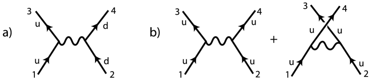
Figure 10: Feynman diagrams for quark-quark scattering: (a) $ud\to ud$, (b) $uu\to uu$.

5.1 Four-fermion processes

Begin with quark-quark scattering. For scattering of quarks of different flavor, there is only one Feynman diagram, shown in Fig. 10(a). The value of this diagram can be found from (26). In this formula, all momenta are outgoing, so we simply need to cross the correct particles into the initial state. Which particles should be crossed depends on which helicity amplitude we are considering, for example, $u_{L}d_{L}\to u_{L}d_{L}$ or $u_{L}d_{R}\to u_{L}d_{R}$. We also need to include the QCD color matrices. With the numbering of lines as in the figure, with the arrows indicating the direction of left-handed fermions, the matrix elements are

$$i{\cal M}(u_{L}d_{L}\to u_{L}d_{L}) = ig^{2}{{\langle 34\rangle}^{2}\over\langle 13\rangle\langle 24\rangle}T^{a}_{31}T^{a}_{42}$$

$$i{\cal M}(u_{L}d_{R}\to u_{L}d_{R}) = -ig^{2}{{\langle 23\rangle}^{2}\over\langle 13\rangle\langle 24\rangle}T^{a}_{31}T^{a}_{42}$$

The scattering of identical quarks, for example, $u_{L}u_{L}\to u_{L}u_{L}$, is given by two Feynman diagrams, shown in Fig. 10(b). For this case

$$i{\cal M}(u_{L}u_{L}\to u_{L}u_{L})=ig^{2}\biggl{[}{{\langle 34\rangle}^{2}\over\langle 13\rangle\langle 24\rangle}T^{a}_{31}T^{a}_{42}-{{\langle 43\rangle}^{2}\over\langle 14\rangle\langle 23\rangle}T^{a}_{41}T^{a}_{32}\biggr{]}\ .$$ (82)

The extra minus sign in the second term comes from interchange of identical fermions. To compute cross sections, we square these expressions, sum over final helicities and colors, and average over initial helicities and colors. The interference term in the square of (82) requires

$$\langle 13\rangle\langle 24\rangle(\langle 14\rangle\langle 23\rangle)^{*}=\langle 13\rangle[32]\langle 24\rangle[41]=-\langle 13\rangle[31]\langle 14\rangle[41]=-tu\ .$$ (83)

By parity, the cross sections are unchanged when all helicities are reversed. The cross sections for antiquarks can be computed by applying crossing symmetry, so the formulae above are all that we need to cover all of the possible cases.

For the color sums and averages, here and in the later calculations in this section, we will need the formula $T^{a}T^{a}={8\over 3}{\bf 1}$ and the traces

$${\mbox{\rm tr}}[T^{a}T^{a}T^{b}T^{b}]={64\over 3}\ ,\quad{\mbox{\rm tr}}[T^{a}T^{b}T^{a}T^{b}]=-{8\over 3}\ .$$ (84)

These are easily proved using (54). The second trace appears in the interference term in the square of (82). For a general $SU(N)$ gauge group, these results are

$${\mbox{\rm tr}}[T^{a}T^{a}T^{b}T^{b}]={(N^{2}-1)^{2}\over N}\ ,\quad{\mbox{\rm tr}}[T^{a}T^{b}T^{a}T^{b}]=-{(N^{2}-1)\over N}\ ,$$ (85)

so that the second color sum is suppressed by $1/N^{2}$. This is an example of the general result that interference terms between different color structure are suppressed by $1/N^{2}$. That result follows from the broad picture of $1/N$ counting presented by ’t Hooft in [18].

Assembling the pieces, we find

$${d\sigma\over d\cos\theta}(ud\to ud) = {2\over 9}{\pi\alpha_{s}^{2}\over s}\biggl{[}{s^{2}+u^{2}\over t^{2}}\biggr{]}$$

$${d\sigma\over d\cos\theta}(uu\to uu) = {2\over 9}{\pi\alpha_{s}^{2}\over s}\biggl{[}{s^{2}+u^{2}\over t^{2}}+{s^{2}+t^{2}\over u^{2}}-{2\over 3}{s^{2}\over tu}\biggr{]}\ ,$$ (86)

where $\theta$ is the scattering angle in the parton-parton center of mass frame. The second of these formulae is to be integrated over $cos\theta>0$ only. Crossing these formulae into other channels,

$${d\sigma\over d\cos\theta}(u\overline{d}\to u\overline{d}) = {2\over 9}{\pi\alpha_{s}^{2}\over s}\biggl{[}{s^{2}+u^{2}\over t^{2}}\biggr{]}$$

$${d\sigma\over d\cos\theta}(u\overline{u}\to u\overline{u}) = {2\over 9}{\pi\alpha_{s}^{2}\over s}\biggl{[}{s^{2}+u^{2}\over t^{2}}+{t^{2}+u^{2}\over s^{2}}-{2\over 3}{u^{2}\over st}\biggr{]}\ .$$ (87)

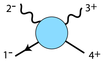
Figure 11: Notation for the process $u_{L}\overline{u}_{R}\to g_{L}g_{R}$.

5.2 $q\overline{q}gg$ processes

Next, consider $q\overline{q}\to gg$. The $q$ and $\overline{q}$ necessarily have opposite helicity. The gluons also have opposite helicity. The two cases of gluon helicity are related by gluon interchange or $t\leftrightarrow u$. So it suffices to consider the case shown in Fig. 11, $u_{L}(4)\overline{u}_{R}(1)\to g_{L}(2)g_{R}(3)$. For this case, the color-ordered amplitudes are MHV amplitudes, and so our results from Section 4 give

$$i{\cal M}=ig^{2}\biggl{[}{{\langle 13\rangle}^{3}\langle 43\rangle\over\langle 12\rangle\langle 23\rangle\langle 34\rangle\langle 41\rangle}T^{a}T^{b}+{{\langle 13\rangle}^{3}\langle 43\rangle\over\langle 13\rangle\langle 32\rangle\langle 24\rangle\langle 41\rangle}T^{b}T^{a}\biggr{]}\ .$$ (88)

The square of this amplitude, traced over color, is

$${\mbox{\rm tr}}[{\cal M}|^{2} = g^{4}\biggl{(}{64\over 3}[{tu\over s^{2}}+{t^{3}\over us^{2}}]-2{8\over 3}{t^{2}\over s^{2}}\biggl{)}$$ (89)

$$= {64\over 3}g^{4}[{t\over u}-{9\over 4}{t^{2}\over s^{2}}]\ .$$

From the first line to the second, I have used $u^{2}+t^{2}=(u+t)^{2}-2ut=s^{2}-2ut$. Adding the case with the two gluons interchanged, and including the factors for averaging over initial colors and helicities, we find as the final result,

$${d\sigma\over d\cos\theta}(u\overline{u}\to gg)={16\over 27}{\pi\alpha_{s}^{2}\over s}\biggl{[}{t\over u}+{u\over t}-{9\over 4}{t^{2}+u^{2}\over s^{2}}\biggr{]}\ .$$ (90)

This formula should be integrated over $\cos\theta>0$ only. Crossing this formula into other channels gives

$${d\sigma\over d\cos\theta}(ug\to ug) = {2\over 9}{\pi\alpha_{s}^{2}\over s}\biggl{[}-{s\over u}-{u\over s}+{9\over 4}{s^{2}+u^{2}\over t^{2}}\biggr{]}$$

$${d\sigma\over d\cos\theta}(gg\to u\overline{u}) = {1\over 12}{\pi\alpha_{s}^{2}\over s}\biggl{[}{t\over u}+{u\over t}-{9\over 4}{t^{2}+u^{2}\over s^{2}}\biggr{]}\ .$$ (91)

5.3 Four-gluon processes

Finally, we need to compute the $gg\to gg$ scattering amplitude. This can be done directly from the formalism we have already developed, but it is useful to add one additional trick.

Extend the gauge group from $SU(N)$ to $U(N)$ by adding an extra generator $T^{0}={{\bf 1}/\sqrt{N}}$. Since the 3- and 4-gluon vertices are proportional to the structure constants $f^{abc}$ and the extra $U(1)$ generator commutes with the $SU(N)$ generators, the additional boson gives no contribution to the cross sections. However, adding this term simplifies the color algebra. The contraction identity (54) now takes the simpler form

$$T^{a}_{ij}T^{a}_{k\ell}=\delta_{i\ell}\delta_{kj}\ .$$ (92)

We can use this identity to compute the square of the 4-gluon amplitude (50). The squares of the individual color traces are equal to

$${\mbox{\rm tr}}[T^{a}T^{b}T^{c}T^{d}]\,{\mbox{\rm tr}}[T^{d}T^{c}T^{b}T^{a}]=N^{4}=81\ .$$ (93)

The cross terms are proportional to

$${\mbox{\rm tr}}[T^{a}T^{b}T^{c}T^{d}]\,{\mbox{\rm tr}}[T^{d}T^{c}T^{a}T^{b}]={\mbox{\rm tr}}[T^{a}T^{b}T^{c}T^{d}]\,{\mbox{\rm tr}}[T^{d}T^{a}T^{b}T^{c}]=N^{2}=9\ .$$ (94)

Then, letting $I,J=1,\ldots,6$ index the six possible cyclic orderings of the gluons, we find

$${\mbox{\rm tr}}[|{\cal M}|^{2}] = 81\sum_{I}|{\bf M}(I)|^{2}+9\sum_{I\neq J}{\bf M}(I){\bf M}(J)^{*}$$ (95)

$$= 72\sum_{I}|{\bf M}(I)|^{2}+9|\sum_{I}{\bf M}(I)|^{2}\ .$$

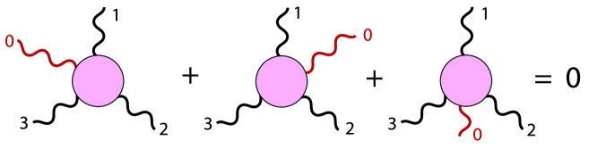
Figure 12: The $U(1)$ Ward identity for color-ordered amplitudes.

I explained above that, when we add the extra generator to extend $SU(N)$ to $U(N)$, the value of ${\mbox{\rm tr}}|{\cal M}|^{2}$ cannot change. The vanishing of the coupling to the $T^{0}$ gauge bosons is expressed in the color-ordered amplitudes as the Ward identity shown in Fig. 12: The sum over all possible orderings of a $U(1)$ boson in a color-ordered $n$-gluon amplitudes must vanish. An example of this identity, for 4-gluon amplitudes, is

$$i{\bf M}(0_{-}1_{-}2_{+}3_{+})+i{\bf M}(1_{-}0_{-}2_{+}3_{+})+i{\bf M}(1_{-}2_{+}0_{-}3_{+})=0$$ (96)

We can easily check this from the explicit expressions for MHV amplitudes. Evaluating the left-hand side of (96) gives

$$ig^{2}{\langle 01\rangle}^{4}\biggl{[}{1\over\langle 01\rangle\langle 12\rangle\langle 23\rangle\langle 30\rangle}+{1\over\langle 10\rangle\langle 02\rangle\langle 23\rangle\langle 31\rangle}+{1\over\langle 12\rangle\langle 20\rangle\langle 03\rangle\langle 31\rangle}\biggr{]}$$

$$=ig^{2}{\langle 01\rangle}^{4}{\bigl{[}\langle 02\rangle\langle 13\rangle+\langle 03\rangle\langle 21\rangle+\langle 01\rangle\langle 32\rangle\bigr{]}\over\langle 01\rangle\langle 12\rangle\langle 23\rangle\langle 30\rangle\langle 02\rangle\langle 13\rangle}$$ (97)

The expression in brackets in the second line vanishes by the Schouten identity (19).

The $U(1)$ Ward identity implies that

$$\sum_{I}{\bf M}(I)=0\ .$$ (98)

Then (95) becomes

$${\mbox{\rm tr}}[|{\cal M}|^{2}]=72\sum_{I}|{\bf M}(I)|^{2}\ .$$ (99)

Now we must evaluate this expression for all possible choices of the external particle helicities. Of the 16 possibilities, only 6 involve 2 positive and 2 negative helicities. All other choices give zero. For the color-ordering $1234$, the nonzero amplitudes are

$$|{\bf M}(1_{-}2_{-}3_{+}4_{+})|^{2} = g^{4}\biggl{|}{{\langle 12\rangle}^{4}\over\langle 12\rangle\langle 23\rangle\langle 34\rangle\langle 41\rangle}\biggr{|}^{2}=g^{4}{s^{2}\over t^{2}}$$

$$|{\bf M}(1_{-}2_{+}3_{-}4_{+})|^{2} = g^{4}\biggl{|}{{\langle 13\rangle}^{4}\over\langle 12\rangle\langle 23\rangle\langle 34\rangle\langle 41\rangle}\biggr{|}^{2}=g^{4}{u^{4}\over s^{2}t^{2}}$$

$$|{\bf M}(1_{-}2_{+}3_{+}4_{-})|^{2} = g^{4}\biggl{|}{{\langle 14\rangle}^{4}\over\langle 12\rangle\langle 23\rangle\langle 34\rangle\langle 41\rangle}\biggr{|}^{2}=g^{4}{t^{2}\over s^{2}}\ ,$$ (100)

and the parity conjugates of these amplitudes. The sum over color orderings sums over these results crossed into all possible channels. Thus

$$\sum_{h}\sum_{I}{\mbox{\rm tr}}|\bf M(I)|^{2} = 4g^{4}\cdot[{s^{2}+u^{2}\over t^{2}}+{t^{2}+u^{2}\over s^{2}}+{s^{2}+t^{2}\over u^{2}}+{u^{4}\over t^{2}s^{2}}+{t^{4}\over u^{2}s^{2}}+{s^{4}\over t^{2}u^{2}}]$$ (101)

$$= 16g^{4}[3-{su\over t^{2}}-{ut\over s^{2}}-{st\over u^{2}}]\ .$$

Including the factors for initial-state color and helicity averaging, we find

$${d\sigma\over d\cos\theta}(gg\to gg)={9\over 4}{\pi\alpha_{s}^{2}\over s}[3-{su\over t^{2}}-{ut\over s^{2}}-{st\over u^{2}}]\ .$$ (102)

This formula should be integrated over $\cos\theta>0$ only. This completes the calculation of all of the tree-level $2\to 2$ parton-parton scattering cross sections.

6 Britto-Cachazo-Feng-Witten recursion

Now I will develop some methods that will allow us to prove the MHV formulae, and also to use these results to compute the more compex non-MHV amplitudes. The general approach will follow the idea of Cachazo, Svrcek, and Witten [19, 20] that we should consider the tree-level color-ordered amplitudes as analytic functions of the angle brackets and square brackets. We can then analytically continue scattering amplitudes to complex momenta while keeping the property that all external legs are on mass shell. At the end of the calculation, to extract physical results, we will specialize to the values such that $\langle ij\rangle=([ji])^{*}$.

6.1 Three-point scattering amplitudes

This freedom to discuss QCD scattering amplitudes for arbitrary complex momenta allows us to write on-shell three-point scattering amplitudes. For three-point amplitudes, shown in Fig. 13, momentum conservation implies that $1+2+3=0$. Then

$$0=1^{2}=(2+3)^{2}=2\,2\cdot 3\ ,$$ (103)

and similarly the other two Lorentz products vanish, so it would seem that there are no invariants for these amplitudes to depend on. However, in terms of square brackets and angle brackets,

$$2\,2\cdot 3=s_{23}=\langle 23\rangle[32]\ .$$ (104)

Thus, with complex momenta, we can satisfy (103) by having $[32]=0$ while keeping $\langle 23\rangle$ nonzero.

Figure 13: Diagrams contributing to the three-point $qg\overline{q}$ and $ggg$ amplitudes.

With this idea in mind, I will compute the color-ordered amplitude for gluon emission from $q\overline{q}$, $i{\bf M}(q_{-}(1)g_{-}(2)\overline{q}_{+}(3))$. The amplitude comes from one Feynman diagram, shown in Fig. 13. The value of this diagram is

$${ig\over\sqrt{2}}\langle 1{\gamma^{\mu}}3]\,(-{1\over\sqrt{2}}{[r{\gamma_{\mu}}2\rangle\over[r2]})\ ,$$ (105)

with $r$ an arbitrary lightlike reference vector. Applying the Fierz identity, and then multiplying top and bottom by $\langle 12\rangle$, this rearranges to

$$-ig{\langle 12\rangle[r3]\langle 21\rangle\over[r2]\langle 21\rangle}=-ig{{\langle 12\rangle}^{2}\over\langle 31\rangle}\ .$$ (106)

The reference vector $r$ cancels out, and the final result is just the MHV amplitude with $n=3$,

$$i{\bf M}(q_{-}(1)g_{-}(2)\overline{q}_{+}(3))=ig{{\langle 12\rangle}^{3}\langle 32\rangle\over\langle 12\rangle\langle 23\rangle\langle 31\rangle}\ .$$ (107)

A similar calculation gives the form of the three-gluon vertex.

$$i{\bf M}(g_{-}(1)g_{-}(2)g_{+}(3))$$

$$\hskip 7.22743pt={ig\over\sqrt{2}}[\epsilon(1)\cdot\epsilon(2)(1-2)\cdot\epsilon(3)$$

$$\hskip 43.36243pt+\epsilon(2)\cdot\epsilon(3)(2-3)\cdot\epsilon(1)+\epsilon(3)\cdot\epsilon(1)(3-1)\cdot\epsilon(2)]\ .$$ (108)

Choose for the polarization vectors

$$\epsilon^{\mu}(1)=-{1\over\sqrt{2}}{[r{\gamma^{\mu}}1\rangle\over[r1]}\ ,\quad\epsilon^{\mu}(2)=-{1\over\sqrt{2}}{[r{\gamma^{\mu}}2\rangle\over[r2]}\ ,\quad\epsilon^{\mu}(3)={1\over\sqrt{2}}{\langle s{\gamma^{\mu}}3]\over\langle s3\rangle}\ ,$$ (109)

so that $\epsilon(1)\cdot\epsilon(2)=0$. Then (108) evaluates to

$${ig\over\sqrt{2}}{1\over\sqrt{2}}{(0+[r3]\langle s2\rangle[r\,(2-3)\,1\rangle+[r3]\langle s1\rangle[r\,(3-1)\,2\rangle)\over[r1][r2]\langle s3\rangle}$$

$$=ig{[r3]\over[r1][r2]\langle s3\rangle}([r3]\langle 31\rangle\langle 2s\rangle-[r3]\langle 32\rangle\langle 1s\rangle)$$

$$=ig{{\langle 12\rangle}{[r3]}^{2}\over[r1][r2]}$$ (110)

If we multiply top and bottom by ${\langle 12\rangle}^{2}$ and rearrange the denominator, the factors of $\langle r3\rangle$ cancel, and we find

$$i{\bf M}(g_{-}(1)g_{-}(2)g_{+}(3))=ig{{\langle 12\rangle}^{4}\over\langle 12\rangle\langle 23\rangle\langle 31\rangle}\ .$$ (111)

For reference, the corresponding formulae for two positive and one negative helicity are

$$i{\bf M}(q_{-}(1)g_{+}(2)\overline{q}_{+}(3))=ig{{[12]}{[32]}^{3}\over[12][23][31]}\ ,\quad i{\bf M}(g_{+}(1)g_{+}(2)g_{-}(3))=-ig{{[12]}^{4}\over[12][23][31]}\ .$$ (112)

I note again that all other $n$-gluon and $q\overline{q}+n$ gluon amplitudes with only one negative or positive helicity are zero. Only these cases are nonzero, with the MHV values.

6.2 BCFW recursion formula

It would be wonderful if we could use these three-point functions as building blocks for the construction of general tree amplitudes. The usual understanding is that we need off-shell three-point functions to build up general amplitudes. However, this common-sense idea is evaded by a beautiful strategy of Britto, Cachazo, Feng, and Witten [21].

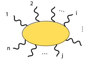
Figure 14: Notation for the discussion of the Britto-Cachazo-Feng recursion formula.

Consider a color-ordered amplitude $i{\bf M}(1\cdots n)$, as shown in Fig. 14. Choose two legs $i$, $j$, and choose a value of $z$, a complex variable. Now define new momenta $\hat{i}$ and $\hat{j}$ by shifting the square bracket of $i$ and the angle bracket of $j$,

$$\hat{i}\rangle=i\rangle\phantom{\ -zi\rangle} \hat{i}]=i]+zj]$$

$$\hat{j}\rangle=j\rangle-zi\rangle \hat{j}]=j]\ ,$$ (113)

The momenta $\hat{i}$ and $\hat{j}$ are given by

$$\hat{i}=i\rangle[i+z\ i\rangle[j\qquad\hat{j}=j\rangle[j-z\ i\rangle[j\ .$$ (114)

Notice that $\hat{i}+\hat{j}=i+j$, so momentum conservation is respected. For general $z$, $\hat{i}$ and $\hat{j}$ have unphysical complex values. However, since $\hat{i}^{2}$ is proportional to $\langle ii\rangle=0$, and similarly, $\hat{j}^{2}=0$, the new momenta remain on shell.

As a rule of thumb, one should shift the square bracket of an external state with negative helicity and the angle bracket of an external state with positive helicity, that is, $(i,j)=(-,+)$. This minimizes the number of factors of $z$ in the numerator. I will give a more careful analysis of this point below.

Call the amplitude evaluated at the modified momenta $i{\bf M}(z)$. Now consider the integral

$$\oint{dz\over 2\pi i}{1\over z}\,i{\bf M}(z)$$ (115)

taken around a large circle in the complex $z$ plane. If $i{\bf M}(z)\to 0$ as $z\to\infty$, then this integral vanishes. In that case, we can set to zero the value obtained by contracting the contour and summing over the poles that it encloses. There is an obvious pole at $z=0$. The residue of this pole is exactly

$$i{\bf M}(z=0)\ ,$$ (116)

the amplitude that we wish to evaluate.

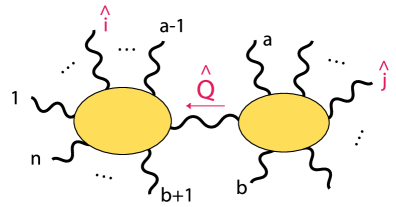
Figure 15: A factorization of the amplitude in Fig. 14 that gives a pole in the amplitude $i{\bf M}(z)$.

The other poles come from the denominator of the color-ordered amplitude. We are discussing tree amplitudes, and so these poles will come from the propagator involved in a factorization of the amplitude, as shown in Fig. 15. The denominator of this propagator is

$$\hat{Q}^{2}=s_{a\cdots b}(z)=\bigl{(}\sum^{b}_{m=a}k_{m}\bigr{)}^{2}\ ,$$ (117)

the invariant sum of momenta on the right, including any terms from the shifts (114). If both $i$ and $j$ are on the same side in the factorization, $s_{a\cdots b}$ is idependent of $z$ and there is no pole. If $i$ is on the left side in the factorization and $j$ is on the right,

$$s_{a\cdots b}(z) = (\ \sum_{m=a}^{b}k_{m}-zi\rangle[j\ )^{2}$$ (118)

$$= s_{a\cdots b}(0)-z\langle i(\sum_{a}^{b}k_{m})j]+z^{2}\langle ii\rangle[jj]\ .$$

The last term is zero. The denominator then has a simple pole at

$$z_{*}={s_{a\cdots b}\over\langle i(\sum_{a}^{b}k_{m})j]}\ .$$ (119)

The residue of this pole is

$${1\over z_{*}}i{\bf M}((b+1)\ldots\hat{i}\ldots(a-1)\hat{Q}){i\over-\langle i(\sum_{a}^{b}k_{m})j]}i{\bf M}(\hat{Q}a\ldots\hat{j}\ldots b)$$

$$=-i{\bf M}((b+1)\ldots\hat{i}\ldots(a-1)\hat{Q}){i\over s_{a\cdots b}}i{\bf M}(\hat{Q}a\ldots\hat{j}\ldots b)$$ (120)

The amplitudes in each term are evaluated with the value $z=z_{*}$, given by (119), appropriate to the cut that is chosen.

The result of this analysis is that, if we have chosen the shifted momenta $i$ and $j$ so that $i{\bf M}(z)$ vanishes at infinity, then

$$i{\bf M}(1\ldots n)=\sum_{a,b}i{\bf M}((b+1)\ldots\hat{i}\ldots(a-1)(-\hat{Q}))\ {i\over s_{a\cdots b}}\ i{\bf M}(\hat{Q}a\ldots\hat{j}\ldots b)\ .$$ (121)

where $Q=-\sum_{a}^{b}k_{m}$. This is the BCFW recursion formula. An arbitrary color-ordered helicity amplitude can then be evaluated by breaking it down into amplitudes with a smaller number of legs. The amplitudes on the right-hand side of (121) are evaluated with on-shell but complex-valued momenta.

The recursion must be run until we can immediately evaluate the amplitudes on the right-hand side. Since all nonzero amplitudes with five external legs or fewer are either MHV or the conjugates of MHV amplitudes, only a few steps of the recursion are needed in practice.

For QCD with all massless particles, the complete solution of the recursion is known. However, the result is not simple, so, in keeping with the philosophy of these lectures, I will refer you to the reference [22, 23, 24]

There is one subtlety that should be clarified to evaluate the right-hand side of the BCFW recursion formula. The amplitudes involve angle brackets and square brackets of the complex momentum $\hat{Q}$. In the examples given later in our discussion, I will evaluate these brackets by assembling them into complete factors of the momentum $\hat{Q}$. To do this, we will need to relate the brackets $(-\hat{Q})\rangle$ and $(-\hat{Q})]$ in the amplitude on the left to $\hat{Q}\rangle$ and $\hat{Q}]$. It is consistent always to take

$$(-\hat{Q})\rangle=i\hat{Q}\rangle\qquad(-\hat{Q})]=i\hat{Q}]\ .$$ (122)

One special circumstance should be noted. If the line on which the amplitude factorizes is a fermion propagator, the value of this propagator is

$$i{Q]\langle Q\over Q^{2}}\quad\mbox{\quad}i{Q\rangle[Q\over Q^{2}}\ .$$ (123)

Then one of the brackets in the left-hand amplitude is a $Q]$, not a $(-Q)]$. To compensate for this, we need to add a factor $(-i)$ for a cut through a fermion propagator.

Finally, we need to discuss under what circumstances the amplitude $i{\bf M}(z)$ will vanish at infinity. I claim that, for the shift given by (113) in which $i$ is shifted in the square bracket and $j$ is shifted in the angle bracket, the helicity choices $(i,j)=(-,+),(-,-),(+,+)$ give the BCFW recursion formula, while in the case $(i,j)=(+,-)$ there are extra terms from the integral at infinity. A transparent argument for this claim has been given by Arkani-Hamed and Kaplan [25].

In the limit $z\to\infty$, the dominant momentum flowing through the diagram is that induced by the shift. Define

$$q=i\rangle[j\ \mbox{or}\ q^{\mu}=\langle i\gamma^{\mu}j]$$ (124)

Then the large momentum is $zq$. Note that $q^{2}=0$. It is useful to picture the diagrams as containing one line whose propagators carry momenta $zq+k$ close to this large momenta. This line attaches to propagators that carry momenta of order 1. This structure is illustrated in Fig. 16. Each propagator has a denominator of order

$$(zq+k)^{2}=2zq\cdot k+k^{2}={\cal O}(z)\ .$$ (125)

Each vertex is at most linear in momentum, and so is at most of order $z$. Then each combination of vertex and propagator is of order $z^{0}$. The chain of vertices and propagators has one extra vertex, so this is of order $z$.

Now consider the polarization vectors. We can choose $i$ or $j$ as the reference vector, whichever gives a nonsingular result. Then

$$\epsilon_{+}(\hat{i})={z\langle j\gamma^{\mu}j]+\langle j\gamma^{\mu}i]\over\langle ji\rangle}+\cdots \epsilon_{-}(\hat{i})=-{1\over z}{[i\gamma^{\mu}i\rangle\over[ij]}$$

$$\epsilon_{+}(\hat{j})=-{1\over z}{\langle j\gamma^{\mu}j]\over\langle ji\rangle} \epsilon_{-}(\hat{j})=-{z\langle i\gamma^{\mu}i]-\langle i\gamma^{\mu}j]\over[ij]}+\cdots\ .$$ (126)

For the choice $(i,j)=(-,+)$, from the $z$-dependence of the polarization vectors and the internal vertices and propagators, we see that the amplitude cannot be larger than ${\cal O}(1/z)$. For the choice $(i,j)=(-,-)$, there is apparently a term of order $z^{1}$. However, it is not possible to build this term, since

$$\epsilon_{-}(\hat{i})\cdot\epsilon_{-}(\hat{j})=0\quad q\cdot\epsilon_{-}(\hat{i})=q\cdot\epsilon_{i}(\hat{j})=0\ .$$ (127)

The first nonzero term is one in which both $\epsilon_{-}(\hat{i})$ and $\epsilon_{-}(\hat{j})$ are dotted with ${\cal O}(1)$ vectors instead of $zq^{\mu}$, and this term is down by two powers of $z$, giving in all an amplitude of of ${\cal O}(1/z)$. An analogous argument holds for the $(+,+)$ case. The amplitude in the $(+,-)$ case is irremediably ${\cal O}(z^{3})$.

A parallel argument can be carried out for the case in which the shifted lines are fermions. In the fermion case, the vertex involves no momenta and is of order $z^{0}$, but the propagator is also ${\cal O}(z^{0})$. The leading term in the propagator is proportional to $\not{\hbox{\kern-2.0pt$q$}}$, which annihilates both $i\rangle$ and $j]$. Then, again, only the $(+,-)$ case can be nonzero as $z\to\infty$. There is one exception to this rule: If we shift on momenta $i$ and $j$ at opposite ends of the same fermion line, the diagrams with only a single vertex and no internal propagators on this line can give a term of ${\cal O}(z^{0})$.

The paper [25], taking a somewhat more sophisticated approach, generalizes this conclusion to other theories, including gravity.

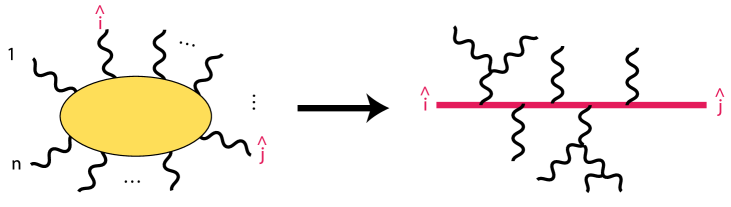
Figure 16: Analysis of the $z\to\infty$ behavior of a multigluon tree diagram.

6.3 Proof of the MHV formula

As a first application of the BCFW recursion formula, I will give a proof of the MHV formula (79) for $n$-gluon amplitudes, using an argument originally given by Risager [26]. The other MHV formulae in Section 4 can be proved by the same method.

The proof will proceed by induction. We have already verified this formula for the $n=3,4$ MHV gluon amplitudes. So, I will assume that the MHV formula is correct for the case $n=N-1$ and use that hypothesis to evaluate the $n=N$ gluon MHV amplitude.

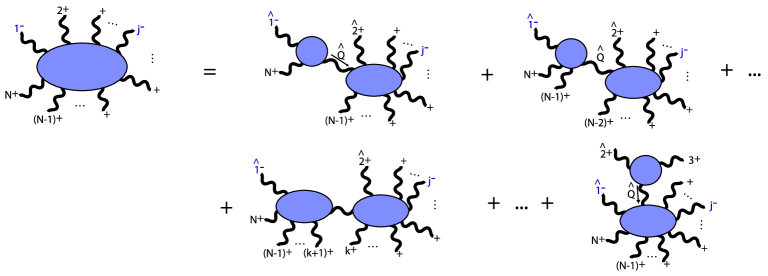
Figure 17: BCFW cuts contributing to the evaluation of the $n$-gluon MHV amplitude.

The $N$-gluon amplitudes are cyclically invariant. So, without loss of generality, choose the gluon 1 to be one of the two gluons with negative helicity. Define the $z$-dependent amplitude in the BCFW procedure by the shift

$$\hat{1}]=1]+z\,2]\qquad\hat{2}\rangle=2\rangle-z\,1\rangle\ .$$ (128)

The BCFW recursion formula then evaluates the $N$-point MHV amplitude in terms of factorized diagrams with $\hat{1}$ on one side of the factorization and $\hat{2}$ on the other, as shown in Fig. 17. In each diagram, we must assign a helicity to the intermediate gluon. There are two choices: $+$ outgoing from one side and $-$ outgoing from the other side, or vice versa. In most cases, both choices give zero, since one side or the other will be an $n$-gluon amplitude with $n>3$ and one or zero $-$ helicity, which vanishes by the arguments given in Section 4. The two diagrams that are potentially nonzero are those in which one side or the other is an amplitude with $n=3$. These are the first and last diagrams in the series shown in Fig. 17.

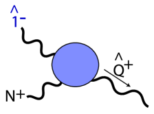
Figure 18: The three-point amplitude from the first diagram in Fig. 17.

The first diagram on the right-hand side in the figure involves the 3-point vertex shown in Fig. 18. The denominator of the exposed propagator is

$$\hat{Q}^{2}=\langle 1N\rangle[N(1+z2)]$$ (129)

However, the 3-point vertex has the form

$$-ig{{[N\hat{Q}]}^{4}\over[\hat{Q}\hat{1}][\hat{1}N][N\hat{Q}]}=+ig[N(1+z2)]\ .$$ (130)

Then vertex cancels the pole in $z$ from the propagator, so the diagram actually has no pole.

The only nonzero contribution to the sum then comes from the last diagram. Its value is

$$ig^{N-3}{{\langle 1j\rangle}^{4}(-1)\over\langle 1\hat{Q}\rangle\langle\hat{Q}4\rangle\langle 45\rangle\cdots\langle N1\rangle}{i\over\langle 23\rangle[32]}(-ig){{[23]}^{4}\over[\hat{Q}2][23][3\hat{Q}]}$$ (131)

with

$$\hat{Q}=-2\rangle[2-3\rangle[3+z1\rangle[2\ .$$ (132)

From (132), we derive

$$\langle 1\hat{Q}\rangle[\hat{Q}3] = -\langle 12\rangle[23]$$

$$\langle 4\hat{Q}\rangle[\hat{Q}2] = -\langle 43\rangle[32]\ .$$ (133)

The factors of $[23]$ all cancel, and we end up with the result

$$ig^{N-2}{{\langle 1j\rangle}^{4}\over\langle 12\rangle\langle 23\rangle\langle 34\rangle\langle 45\rangle\cdots\langle N1\rangle}$$ (134)

which is exactly the Parke-Taylor amplitude for the case of $n=N$ legs. By induction, this formula applies for all $n$.

The MHV formula for $n$-gluon amplitudes with 2 $+$ helicities, and the MHV formulae for amplitudes with 2 fermions and $(n-2)$ gluons can be proved by following the same strategy.

7 $pp\to W^{+}$ + partons

As an illustration of this technology, I will now derive the complete set of formulae needed to compute the cross section for vector boson production with up to 2 partons at a hadron collider. The methods I have discussed make the computation of the cross section for a vector boson plus one parton truly trivial. Only some particular 2 parton amplitudes will require a little work.

For definiteness, I will write formulae for $W^{+}$ production from $u$ and $d$ quarks. The contributions from other light flavors, and the corresponding formulae for $W^{-}$ and $Z^{0}$ production, can be derived from these by small modifications of the prefactors.

7.1 $u\overline{d}\to W^{+}$

The coupling of the $W^{+}$ to quarks and leptons is

$$\delta{\cal L}={g_{w}\over\sqrt{2}}W^{-}_{\mu}(\overline{d}\gamma^{\mu}P_{L}u+\overline{\ell}\gamma^{\mu}P_{L}\nu)+h.c.\ ,$$ (135)

where $P_{L}=(1-\gamma^{5})/2$ is the left-handed projector, and $g_{w}$ is the weak interaction coupling, satisfying

$$\alpha_{w}={g_{w}^{2}\over 4\pi}={1\over 29.6}\ .$$ (136)

The $W^{-}$ field appears because this is the field that creates the $W^{+}$. This interaction leads to an amplitude given by the Feynman diagram shown in Fig. 19

$$i{\cal M}(u\overline{d}\to\nu\ell^{+}) = i{g_{w}^{2}/2\over s_{12}-m_{W}^{2}+im_{W}\Gamma_{W}}\overline{u}(1)\overline{\sigma}^{\mu}u(2)\,\overline{u}(3)\overline{\sigma}_{\mu}u(4)$$ (137)

$$= ig_{w}^{2}{1\over s_{12}-m_{W}^{2}+im_{W}\Gamma_{W}}\langle 31\rangle[24]\ .$$

We can treat this formula in one of two ways. One way is to integrate over the full phase space of the final-state leptons. This will give a broad mass distribution for the leptons, on top of which the $W^{+}$ will appear as a resonance.

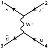
Figure 19: Feynman diagrams for $u\overline{d}\to\nu\ell^{+}$.

Alternatively, since the $W^{+}$ is a narrow resonance, it is typically a good approximation to compute amplitudes for a real $W^{+}$ boson on its mass shell. In this case, you might think it is easiest to sum over the $W^{+}$ polarization vectors. However, we will obtain simpler formulae if we retain the final-state lepton spinors. As a bonus, retaining the spinors will preserve the information on the $W^{+}$ polarization. This is valuable, first, because the $W^{+}$ polarization gives useful information on the dynamics of the $W^{+}$ production and, second, because the experimental acceptance for a $W^{+}$ depends strongly on its polarization.

The matrix element for the $W^{+}$ coupling to leptons is proportional to the current $\overline{u}(\nu)\overline{\sigma}^{\mu}v(\ell^{+})$. This matrix element must be squared and integrated over the direction of the leptons in the $W^{+}$ rest frame. That integral is

$$I^{\mu\nu}=\int{d\Omega\over 4\pi}\ \langle 1{\gamma^{\mu}}2]\langle 2\gamma^{\nu}1]\ .$$ (138)

To evaluate this integral, note that, if $q^{\mu}$ is the $W^{+}$ momentum, $q=1+2$, then $q_{\mu}I^{\mu\nu}=q_{\nu}I^{\mu\nu}=0$. Further,

$$I^{\mu}{}_{\mu}=\int{d\Omega\over 4\pi}\ 2\langle 12\rangle[12]=-2q^{2}=-2m_{W}^{2}\ .$$ (139)

From these requirements,

$$I^{\mu\nu}=-{2\over 3}m_{W}^{2}(g^{\mu\nu}-{q^{\mu}q^{\nu}\over m_{W}^{2}})\ .$$ (140)

The quantity in parentheses in this equation is the usual sum over on-shell $W^{+}$ polarization vectors. Thus we can represent this sum as

$$\sum_{i}\epsilon_{i}^{\mu}(q)\epsilon_{i}^{*\nu}(q)={3\over 2m_{W}^{2}}\int{d\Omega\over 4\pi}\ \langle 1{\gamma^{\mu}}2]\langle 2\gamma^{\nu}1]\ .$$ (141)

This gives a simple procedure for computing cross sections with a final on-shell $W^{+}$ [15]: (1) Write the Feynman diagrams with an internal $W^{+}$ propagator and the final state $\nu(1)\ell^{+}(2)$. (2) Remove the factor $(g_{w}/\sqrt{2})/(s_{12}-m_{W}^{2}+im_{W}\Gamma_{W})$ and put the $W^{+}$ momentum (1+2) on shell.  (3) Evaluate the amplitude with spinor products. (4) Square and integrate over phase space including the on-shell $W^{+}$, and add an integral over the lepton direction in the $W^{+}$ rest frame:

$$\int d\Pi_{n+W}\equiv\int d\Pi_{n+1}{3\over 2m_{W}^{2}}\int{d\Omega\over 4\pi}\ .$$ (142)

The cross section for $W^{+}$ production is typically already a multi-dimensional Monte Carlo integral, so the computational price of adding two additional, well-behaved integrals is small.

To illustrate this formalism, I will work out the cross section for $u\overline{d}\to W^{+}$. I use the matrix element (137) in the form

$$i{\cal M}(W^{+}d\overline{u})={g_{w}\over\sqrt{2}}\langle 1\gamma^{\mu}2]\langle 3\gamma^{\mu}4]=\sqrt{2}g_{w}\langle 31\rangle[24]\ .$$ (143)

The phase space integral $\int d\Pi_{0+W}$ contains 1-body phase space

$$\int d\Pi_{1}=2\pi\delta(s-m_{W}^{2})\ .$$ (144)

Then, averaging over initial colors and spins, we find

$$\sigma(u\overline{d}\to W^{+})={1\over 3\cdot 4}\cdot{8\pi\alpha_{w}\over 2s}\cdot 2\pi\delta(s-m_{W}^{2})\cdot{3\over 2m_{W}^{2}}\int{d\Omega\over 4\pi}\ s_{24}^{2}\ .$$ (145)

The integral over $d\Omega$ implements the familiar $(1-\cos\theta)^{2}$ angular distribution of the decay lepton with respect to the $u$ quark direction, signalling a $W^{+}$ with left-handed polarization. Evaluating the integral, we find

$$\sigma(u\overline{d}\to W^{+})={\pi^{2}\alpha_{w}\over 3}\delta(s-m_{w}^{2})\ ,$$ (146)

the familiar expression for the Drell-Yan cross section.

7.2 MHV amplitudes

To use this formalism for computing $W^{+}$ production cross sections, we need to be able to compute the amplitudes. We might hope that many of these amplitudes belong to an MHV series and are therefore trivial to evaluate. In fact, it is so.

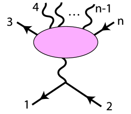
Figure 20: Notation for the amplitudes for $e^{+}_{R}e^{-}_{L}\to q_{L}+ng+\overline{q}_{R}$.

To explain this, I will first compute some amplitudes for the related process $e^{+}e^{-}\to q\overline{q}+ng$. We have seen the first of these, for zero gluons, already in (26) and (28). This amplitude seems to belong to both an MHV and an anti-MHV series. For convenience, I will renumber the external legs to correspond better to the formalism that we used in Section 4. On the electron side, I will take the outgoing left-handed line (the incoming $e^{+}_{R}$) to be line 1; on the quark side, I will take the outgoing left-handed line (the outgoing $q_{L}$) to be line 3. I will notate a general amplitude for $e^{+}_{R}e^{-}_{L}\to q_{L}+ng+\overline{q}_{R}$ in the same way, as shown in Fig. 20. Then the $n=0$ case gives

$$i{\cal M}=-2ie^{2}{{\langle 13\rangle}^{2}\over\langle 12\rangle\langle 34\rangle}=-2ie^{2}{{[24]}^{2}\over[12][34]}\ .$$ (147)

The electric charges gives an additional factor $(-Q_{f})$; I omit this here and in the following.

It is not difficult to work out the next case, $n=5$ or 1 gluon, using the methods described in this review. In the case of a $+$ helicity gluon, it is easiest to take the reference vector for the gluon (line 4) to be 3; for a $-$ helicity gluon, take the reference vector to be 4. Then one finds

$$i{\cal M}(e_{-}(1)\overline{e}_{+}(2)q_{-}(3)g_{+}(4)\overline{q}_{+}(5)) = -2ie^{2}g_{s}{{\langle 13\rangle}^{2}\over\langle 12\rangle\langle 34\rangle\langle 45\rangle}$$

$$i{\cal M}(e_{-}(1)\overline{e}_{+}(2)q_{-}(3)g_{-}(4)\overline{q}_{+}(5)) = 2ie^{2}g_{s}{{[24]}^{2}\over[12][34][45]}\ ,$$ (148)

times the factor $(-Q_{f})$ and the color matrix $T^{a}$. The sum of the squares of these expressions gives

$$\sum|{\cal M}|^{2}=4e^{4}g_{s}^{2}\ {s_{13}^{2}+s_{24}^{2}\over s_{12}s_{34}s_{45}}\ .$$ (149)

This reaction is usually described using the kinematic variables

$$x_{q}={2k_{3}\cdot q\over q^{2}}\ ,\quad x_{g}={2k_{4}\cdot q\over q^{2}}\ ,\quad x_{\overline{q}}={2k_{5}\cdot q\over q^{2}}\ ,$$ (150)

where $q=3+4+5=-(1+2)$. Each $x_{i}$ is the ratio of that particle’s momentum in the center of mass frame to its maximum value $q^{0}/2$. Also,

$$s_{34}=q^{2}(1-x_{\overline{q}})\ ,\quad s_{45}=q^{2}(1-x_{q})\ ,\quad s_{35}=q^{2}(1-x_{g})\ .$$ (151)

The standard expression for the cross section for gluon production in $e^{+}e^{-}$ is

$${d\sigma\over dx_{q}dx_{\overline{q}}}={4\pi\alpha^{2}\over 3s}\cdot 3Q_{f}^{2}\cdot{2\alpha_{s}\over 3\pi}\cdot{x_{q}^{2}+x_{\overline{q}}^{2}\over(1-x_{q})(1-x_{\overline{q}})}\ .$$ (152)

The last factor is almost exactly of the form of (149) after substituting (150), (151). By reintroducing $Q_{f}$, summing over final colors, averaging over helicities, and averaging over the relative orientation of the final state plane with respect to the beam axis, it is not difficult to complete the derivation of (152) from (149).

It is tempting to guess that the formulae (148) generalize to the color-ordered amplitudes for all $+$ helicity and all $-$ helicity gluons according to

$$i{\cal M}(e_{-}(1)\overline{e}_{+}(2)q_{-}(3)g_{+}(4)\cdots g_{+}(n-1)\overline{q}_{+}(n))$$

$$\hskip 144.54pt=-2ie^{2}g_{s}^{n-4}{{\langle 13\rangle}^{2}\over\langle 12\rangle\langle 34\rangle\langle 45\rangle\cdots\langle(n-1)n\rangle}$$

$$i{\cal M}(e_{-}(1)\overline{e}_{+}(2)q_{-}(3)g_{-}(4)\cdots g_{-}(n-1)\overline{q}_{+}(n))$$

$$\hskip 115.63243pt=(-1)^{n+1}2ie^{2}g_{s}^{n-4}{{[2n]}^{2}\over[12][34][45]\cdots[(n-1)n]}\ .$$ (153)

This is in fact correct. These new MHV formulae can be proved using the method of Section 6.3.

Finally, we need to make the connection between the QED amplitudes given here and the amplitudes that we need for $W^{+}$ production. The only change needed is to substitute the photon propagator with a $W^{+}$ propagator by multiplying by the factor

$${g_{w}^{2}\over 2e^{2}}{s_{12}\over s_{12}-m_{W}^{2}+im_{W}\Gamma_{W}}\ ,$$ (154)

and then to take the $W^{+}$ on-shell according to the prescription given below (141). I will write the on-shell amplitudes in the form

$$i{\cal M}(W^{+}(12);3\cdots n) = \sqrt{2}g_{w}g_{s}^{n-4}T^{a_{1}}\cdots T^{a_{n}}\cdot i{\bf M}(12;34\cdots(n+4))$$ (155)

$$\hskip 144.54pt+\mbox{other\ color\ structures}\ .$$

Then for the cases discussed above,

$${\bf M}(12;3\cdots n)=\cases{\phantom{(-1)^{n}}{[12]{\langle 13\rangle}^{2}/\langle 12\rangle\langle 34\rangle\langle 45\rangle\cdots\langle(n-1)n\rangle}&MHV\cr(-1)^{n}{\langle 12\rangle{[2n]}^{2}/[12][34][45]\cdots[(n-1)n]}&anti-MHV\cr}\ .$$ (156)

7.3 $W^{+}$ + 1 parton

The amplitude for $u\overline{d}\to W^{+}+g_{+}$ contains only one color factor. The corresponding color-ordered amplitude, following from (148) or (156), is

$${\bf M}={[12]{\langle 13\rangle}^{2}\over\langle 34\rangle\langle 45\rangle}\ .$$ (157)

Using this result, it is straightforward to compute the lowest-order cross section for production of $W^{+}$ + 1 parton. There are three processes that must be considered:

$$u\overline{d}\to W^{+}g\ ,\quad ug\to W^{+}d\ ,\quad g\overline{d}\to W^{+}\overline{u}\ .$$ (158)

For all three processes, the amplitude is an appropriate crossing of that given in (157).

For $u\overline{d}\to W^{+}g$, after averaging over initial colors and helicities and summing over final colors and helicities, we find

$$\sigma(u\overline{d}\to W^{+}g) = {32\over 9}{\pi^{2}\alpha_{w}\alpha_{s}\over s}\int d\Pi_{1+W}\$$ (159)

$$\hskip 3.61371pt\biggl{\{}|{\bf M}(12;d(3)g_{+}(4)\overline{u}(5)|^{2}+|{\bf M}(12;d(3)g_{-}(4)\overline{u}(5)|^{2}\biggr{\}}\ .$$

I have used the color sum

$${\mbox{\rm tr}}[T^{a}T^{a}]=8\ .$$ (160)

If $\theta_{*}$ is the polar angle in the $W^{+}g$ center of mass system,

$$\int d\Pi_{1+W}={3\over 16\pi m_{W}^{2}}\int{d\cos\theta_{*}\over 2}\int{d\Omega\over 4\pi}\bigl{(}1-{m_{W}^{2}\over s}\bigr{)}$$ (161)

with $s=s_{5}$, and

$$|{\bf M}(12;d(3)g_{+}(4)\overline{u}_{+}(5)|^{2}+|{\bf M}(12;d_{-}(3)g_{-}(4)\overline{u}_{+}(5)|^{2}={s_{13}^{2}+s_{25}^{2}\over s_{34}s_{45}}\ .$$ (162)

Then

$$\sigma(u\overline{d}\to W^{+}g)={2\pi\alpha_{w}\alpha_{s}\over 3s}\int{d\cos\theta_{*}\over 2}\int{d\Omega\over 4\pi}(1-{m_{W}^{2}\over s})\biggl{(}{s_{1d}^{2}+s_{2u}^{2}\over s_{dg}s_{gu}}\biggr{)}\ .$$ (163)

Similarly,

$$\sigma(ug\to W^{+}d)=\sigma(g\overline{d}\to W^{+}\overline{u})={\pi\alpha_{w}\alpha_{s}\over 4s}\int{d\cos\theta_{*}\over 2}\int{d\Omega\over 4\pi}(1-{m_{W}^{2}\over s})\biggl{(}{s_{1d}^{2}+s_{2u}^{2}\over s_{dg}s_{gu}}\biggr{)}\ .$$ (164)

where the $s_{ij}$ invariants are evaluated with appropriately crossed momenta. In the two cases, respectively, $s_{gu}=s$ and $s_{dg}=s$.

7.4 Cross section formulae for $W^{+}$ + 2 partons

For the case of $W$ + 2 partons, many reactions must be included, and each of these has a nontrivial color structure. The reactions are all of the form (2 partons) $\to$ (2 partons) $+W^{+}$, and so they are in 1-to-1 correspondence with the 2-to-2 parton processes that we considered in Section 5. Further, since the $W^{+}$ is a color singlet, the color structure and color sums are also just those that we met in Section 5, and we can borrow the color algebra from that discussion. This will allow us to write the cross sections in terms of the matrix elements ${\bf M}$ normalized as in (155).

We can begin with 4-fermion reactions. For the simplest case of a non-identical spectator quark, the cross section is given in terms of the amplitude ${\bf M}(12;34;56)$ containing three fermion lines: the leptons (12), the left-handed quark emitting the $W^{+}$ (34), and a second left-handed quark (56). This cross section is

$$\sigma(us\to W^{+}ds)={1\over 9}{\alpha_{w}\alpha_{s}^{2}\over s}\cdot 128\pi^{3}\,\int d\Pi_{2+W}\ \biggl{\{}|{\bf M}(12;34;56)|^{2}+|{\bf M}(12;34;65)|^{2}\biggr{\}}\ ,$$ (165)

The sum of matrix elements takes care of the polarization sum for the spectator quark. For spectators identical to the final quark,

$$\sigma(ud\to W^{+}dd) = {1\over 9}{\alpha_{w}\alpha_{s}^{2}\over s}\cdot 128\pi^{3}\,\int d\Pi_{2+W}$$ (166)

$$\hskip-7.22743pt\biggl{\{}|{\bf M}(12;34;56)|^{2}-{1\over 3}{\rm Re}[{\bf M}(12;34;56)^{*}{\bf M}(12;54;36)]$$

$$\hskip 72.26999pt+|{\bf M}(12;34;65)|^{2}]\biggr{\}}\ .$$

I have adjusted the normalization so that the integral can be taken over all of phase space. The cross section $\sigma(uu\to W^{+}du)$ involves a similar sum over matrix elements. Cross sections involving antiquarks have the same form, except that the amplitudes ${\bf M}(12;34;56)$ should be crossed appropriately.

The cross section for the reaction $u\overline{d}\to W^{+}+2g$ is given, analogously to (90), by

$$\sigma(u\overline{d}\to W^{+}gg) = {8\over 27}{\alpha_{w}\alpha_{s}^{2}\over s}\cdot 128\pi^{3}\,\int d\Pi_{2+W}\sum_{ij}$$ (167)

$$\hskip-28.90755pt\biggl{\{}|{\bf M}(12;34_{i}5_{j}6)|^{2}-{1\over 8}{\rm Re}[{\bf M}(12;34_{i}5_{j}6)^{*}{\bf M}(12;35_{j}4_{i}6)]\biggr{\}}\ ,$$

where $i,j=+,-$ are the helicity states of the final gluons. The cross section is again normalized to be integrated over all of phase space. The cross sections with initial-state gluons are given by

$$\sigma(ug\to W^{+}ug) = {1\over 9}{\alpha_{w}\alpha_{s}^{2}\over s}\cdot 128\pi^{3}\,\int d\Pi_{2+W}\sum_{ij}$$

$$\hskip-72.26999pt\biggl{\{}|{\bf M}(12;34_{i}5_{j}6)|^{2}+|{\bf M}(12;35_{j}4_{i}6)|^{2}-{1\over 4}{\rm Re}[{\bf M}(12;34_{i}5_{j}6)^{*}{\bf M}(12;35_{j}4_{i}6)]\biggr{\}}$$

$$\sigma(gg\to W^{+}d\overline{u}) = {1\over 24}{\alpha_{w}\alpha_{s}^{2}\over s}\cdot 128\pi^{3}\,\int d\Pi_{2+W}\sum_{ij}$$ (168)

$$\hskip-93.95122pt\biggl{\{}|{\bf M}(12;34_{i}5_{j}6)|^{2}+|{\bf M}(12;35_{j}4_{i}6)|^{2}-{1\over 4}{\rm Re}[{\bf M}(12;34_{i}5_{j}6)^{*}{\bf M}(12;35_{j}4_{i}6)]\biggr{\}}\ ,$$

where the matrix elements ${\bf M}(12;3456)$ are crossed appropriately.

There is no analogue of the $gg\to gg$ process, since at tree level the $W^{+}$ does not couple directly to gluon lines. So now we have all of the cross section formulae, and it only remains to compute the amplitudes.

7.5 Amplitudes for $W^{+}$ + 2 partons

The cross section formulae in the previous section involve two sets of amplitudes, those for $Wqgg\overline{q}$ and those for $Wq\overline{q}q\overline{q}$. These must be evaluated for all cases of the final-state helicity. However, each quark line must have a left-handed fermion at one end and a right-handed fermion on the other end, so the cases that must be considered are only those of different gluon helicities. Of these, two are MHV or anti-MHV, so only two amplitudes with gluons, plus the four-fermion case, need to be computed. All of those computations are easily done by the BCFW method.

The two amplitudes that are trivially known are:

$${\bf M}(12;d_{-}(3)g_{+}(4)g_{+}(5)\overline{u}_{+}(6)) = {[12]{\langle 13\rangle}^{2}\over\langle 34\rangle\langle 45\rangle\langle 56\rangle}$$

$${\bf M}(12;d_{-}(3)g_{-}(4)g_{-}(5)\overline{u}_{+}(6)) = {\langle 12\rangle{[26]}^{2}\over[34][45][56]}\ .$$ (169)

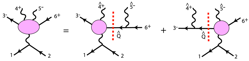
Figure 21: Evaluation of the amplitude $i{\bf M}(12;d_{-}(3)g_{+}(4)g_{-}(5)\overline{u}_{+}(6))$ by BCFW recursion.

I will now take up the case of the amplitude $i{\bf M}(12;d_{-}(3)g_{+}(4)g_{-}(5)\overline{u}_{+}(6))$. To evaluate this amplitude, carry out a BCFW shift on the legs 5 (with square brackets) and 4 (with angle brackets, according to

$$\hat{5}]=5]+z\ 4]\ ,\qquad\hat{4}\rangle=4\rangle-z\ 5\rangle\ .$$ (170)

Then the BCFW recursion formula gives the identity shown in Fig. 21. The vertical dashed lines show the two BCFW cuts.

I will evaluate the first of these cuts explicitly. The amplitude to the left is an MHV amplitude for $Wug\overline{d}$. The amplitude to the right is a nonzero MHV 3-point vertex. Together, these give

$${[12]{\langle 13\rangle}^{2}\over\langle 3\hat{4}\rangle\langle\hat{4}(-\hat{Q})\rangle}\cdot(-i)\cdot{i\over s_{56}}\cdot i{{\langle\hat{Q}\hat{5}\rangle}^{3}\langle 6\hat{5}\rangle\over\langle\hat{Q}\hat{5}\rangle\langle\hat{5}6\rangle\langle 6\hat{Q}\rangle}\ .$$ (171)

The factor $(-i)$ is associated with the fermion cut; see below (123). Using $\hat{5}\rangle=5\rangle$ and $-Q\rangle=iQ\rangle$, this simplifies to

$$-{[12]{\langle 13\rangle}^{2}{\langle 5\hat{Q}\rangle}^{2}\over\langle 3\hat{4}\rangle s_{56}\langle\hat{4}\hat{Q}\rangle\langle 6\hat{Q}\rangle}\ .$$ (172)

The momentum $\hat{Q}$ takes the value

$$\hat{Q}=\hat{Q}\rangle[\hat{Q}=-5\rangle[5-6\rangle[6-z\ 5\rangle[4\ .$$ (173)

This should be evaluated at the value $z=z_{*}$ for which $\hat{Q}^{2}=0$. That is,

$$z_{*}=-{s_{56}\over\langle 5(5+6)4]}=-{[65]\over[64]}\ .$$ (174)

To evaluate the angle brackets of $\hat{Q}$, multiply (172) by ${[\hat{Q}4]}^{2}/{[\hat{Q}4]}^{2}$ and use (173) to evaluate $\hat{Q}\rangle[\hat{Q}$. This gives the identities

$$\langle 5\hat{Q}\rangle[\hat{Q}4] = -\langle 56\rangle[64]$$

$$\langle 6\hat{Q}\rangle[\hat{Q}4] = -\langle 65\rangle[54]$$

$$\langle 4\hat{Q}\rangle[\hat{Q}4] = -(s_{45}+s_{46}+s_{56})=-s_{456}$$ (175)

Also, using (174),

$$\langle 3\hat{4}\rangle=\langle 3(4+5)6]/[46]\ .$$ (176)

With all of these simplifications, the expression for the cut becomes

$${[12]{\langle 13\rangle}^{2}{[46]}^{3}\over[45][56]s_{456}\langle 3(4+5)6]}\ .$$ (177)

After evaluating the second cut in the same way, we arrive at the following expression for the amplitude:

$${\bf M}(12;d_{-}(3)g_{+}(4)g_{-}(5)\overline{u}_{+}(6))=\biggl{\{}{[12]{\langle 13\rangle}^{2}{[46]}^{3}\over[45][56]s_{456}\langle 3(4+5)6]}+{\langle 12\rangle{[26]}^{2}{\langle 35\rangle}^{3}\over\langle 34\rangle\langle 45\rangle s_{345}\langle 3(4+5)6]}\biggr{\}}\ .$$ (178)

The final result is properly symmetric under complex conjugation and interchange of $3\leftrightarrow 6$, $4\leftrightarrow 5$. Notice that the separate terms of the amplitude are singular not only at physical singularities where denominators vanishes, such as $s_{45}=0$, but also on the plane where $\langle 3(4+5)6]=0$. Fortunately, this latter singularity can be shown to cancel between the two terms of the expression.

The two remaining amplitudes can be evaluated by the same technique. For the remaining $Wugg\overline{d}$ amplitude, shifting on 4 and 5 gives

$${\bf M}(12;d_{-}(3)g_{-}(4)g_{+}(5)\overline{u}_{+}(6))=\biggl{\{}{\langle 12\rangle{[46]}{[2(5+6)4\rangle}^{2}\over\langle 45\rangle\langle 56\rangle s_{456}[3(4+5)6\rangle}+{[12][35]{\langle 1(3+4)5]}^{2}\over[34][45]s_{345}[3(4+5)6\rangle}\biggr{\}}\ .$$ (179)

For the 4-fermion amplitude, shifting on 3 and 6 gives

$${\bf M}(12;d_{-}(3)\overline{u}_{+}(4);s_{-}(5)\overline{s}_{+}(6))=-\biggl{\{}{\langle 12\rangle{[24]}^{2}{\langle 35\rangle}^{2}\over\langle 56\rangle s_{356}[4(5+6)3\rangle}-{[12]{\langle 13\rangle}^{2}{[46]}^{2}\over[56]s_{123}[4(5+6)3\rangle}\biggr{\}}\ .$$ (180)

In this case, one should resist the temptation to shift on the lines 5 and 6. That gives a simpler expression, which, however, is not actually correct, because the limit $z\to\infty$ in the BCFW construction does not vanish. Alternatively, the 4-fermion amplitude can be computed very simply directly from the Feynman diagrams using only the technology of Section 2. The result is

$${\bf M}(12;d_{-}(3)\overline{u}_{+}(4);s_{-}(5)\overline{s}_{+}(6))=-\biggl{\{}{\langle 35\rangle[6(3+5)1\rangle[24]\over s_{56}s_{356}}+{\langle 31\rangle[2(1+3)5\rangle[64]\over s_{56}s_{123}}\biggr{\}}\ .$$ (181)

which can be shown to be equal to (180).

In principle, one could go further to amplitudes with $W^{+}$ and any number of quarks and gluons. In practice, it is possible to avoid even writing these expression explicitly. It is quite straightforward to implement the BCFW recursion in a recursive computer algorithm [27]. Then these and higher expressions for amplitudes would be generated automatically starting from the MHV and anti-MHV amplitudes. Alternatively, these higher point amplitudes are computed in [23, 24].

8 Conclusions

In these lectures, I have given an introduction to a set of tools for computing multi-parton tree level amplitudes in QCD. Already at the level of this review, we have seen that calculations that would be tremendously difficult by textbook methods become accessible, or even easy, using the simplifications of spinor products, color ordering, and BCFW recursion. For loop diagrams, even more powerful methods are available, as you might glean from the references. I hope that this review will put you on the road to a better understanding of QCD that will be useful to you in the era of LHC physics.

Appendix A Direct computation of spinor products

In numerical computations with spinor products, it is best to evaluate the spinor products directly from 4-vectors, without first computing vector products. The advantage is not only in speed of execution. In the case where two lightlike vectors are almost collinear, separated by a small angle $\theta$, the vector product vanishes as $\theta^{2}$ while the spinor product vanishes only as $\theta^{1}$. In such a case, working directly with the spinor product avoids round-off error [15].

To evaluate the spinor products of lightlike vectors A and B, first let

$$\eta_{A}=\cases{1&$A^{0}>0$\cr-i&$A^{0}<0$\cr}$$ (182)

Let

$$A^{+}=A^{0}+A^{1}\qquad B^{+}=B^{0}+B^{1}\ .$$ (183)

$$\langle AB\rangle=\eta_{A}\eta_{B}{(A^{3}-iA^{2})B^{+}-(B^{3}-iB^{2})A^{+}\over\sqrt{\eta^{2}_{A}\eta^{2}_{B}A^{+}B^{+}}}$$ (184)

and $[AB]=-(\langle AB\rangle)^{*}$.

In this definition, the axis $\hat{1}$ has a preferred role. In compensation, the spinor product has a singularity in its phase when one of the vectors $A$, $B$ approaches the $-\hat{1}$ direction. This phase choice cancels out of the squares of matrix elements, so any other axis may be used. If the preferred axis is a natural axis of the problem such as the beam direction, one will frequently encounter 0/0 in numerical evaluations. If the beam axis is the $\hat{3}$ direction, it is useful to choose the $\hat{1}$ direction as the preferred axis. Then, working in double precision, excessively small denominators appear only for about 1 point in $10^{6}$; in a Monte Carlo integration, one can trap for and ignore these points.

ACKNOWLEDGEMENTS

I am grateful to Maria Elena Tejeda-Yeomans and Alejandro Ayala for the invitation to present this material in Sonora and for their kind hospitality. I thank Yu-Ping Kuang, Qing Wang, and Hong-Jian He for the invitation to speak at Tsinghua University and for gracious hospitality during my stay in Beijing. I am grateful to Zvi Bern, Sally Dawson, and Lance Dixon, and Daniel Maitre for discussions of these topics. I thank the many students who have helped me understand this material and have critiqued my lectures, in particular, Kassahun Betre, Camile Boucher-Veronneau, Shao-Feng Ge, Xiomara Gutierrez, Andrew Larkoski, and My Phuong Le, This work was supported by the US Department of Energy under contract DE–AC02–76SF00515.

References

- [1] C. F. Berger et al., Phys. Rev. Lett. 102, 222001 (2009) [arXiv:0902.2760 [hep-ph]], Phys. Rev. D 80, 074036 (2009) [arXiv:0907.1984 [hep-ph]]. C. F. Berger, Z. Bern, L. J. Dixon et al., [arXiv:1009.2338 [hep-ph]].
- [2] R. Keith Ellis, K. Melnikov and G. Zanderighi, Phys. Rev. D 80, 094002 (2009) [arXiv:0906.1445 [hep-ph]].
- [3] M. L. Mangano and S. J. Parke, Phys. Rept. 200, 301 (1991) [arXiv:hep-th/0509223].
- [4] L. J. Dixon, arXiv:hep-ph/9601359.
- [5] Z. Bern, L. J. Dixon and D. A. Kosower, Annals Phys. 322, 1587 (2007) [arXiv:0704.2798 [hep-ph]].
- [6] C. F. Berger, D. Forde, Ann.Rev.Nucl.Part.Sci. 60, 181 (2010). [arXiv:0912.3534 [hep-ph]].
- [7] J. Alwall et al., JHEP 0709, 028 (2007) [arXiv:0706.2334 [hep-ph]].
-
[8]
http://madgraph.phys.ucl.ac.be/ - [9] T. Gleisberg, S. .Hoeche, F. Krauss et al., JHEP 0902, 007 (2009). [arXiv:0811.4622 [hep-ph]].
-
[10]
http://projects.hepforge.org/sherpa/dokuwiki/doku.php - [11] T. Gleisberg, S. Hoeche, JHEP 0812, 039 (2008). [arXiv:0808.3674 [hep-ph]].
- [12] F. A. Berends, R. Kleiss, P. De Causmaecker, R. Gastmans and T. T. Wu, Phys. Lett. B 103, 124 (1981); F. A. Berends, R. Kleiss, P. De Causmaecker, R. Gastmans, W. Troost and T. T. Wu [CALKUL Collaboration], Nucl. Phys. B 206, 61 (1982), B 239, 395 (1984), B 239, 382 (1984). B 264, 243, 265 (1986).
- [13] Z. Xu, D. H. Zhang and L. Chang, Tsinghua University preprints TUTP-84/3,4,5a (1984), Nucl. Phys. B 291, 392 (1987).
- [14] J. F. Gunion and Z. Kunszt, Phys. Lett. B 161, 333 (1985).
- [15] R. Kleiss and W. J. Stirling, Nucl. Phys. B 262, 235 (1985).
- [16] C. Schwinn and S. Weinzierl, JHEP 0704, 072 (2007) [arXiv:hep-ph/0703021].
- [17] S. J. Parke and T. R. Taylor, Phys. Rev. Lett. 56, 2459 (1986).
- [18] G. ’t Hooft, Nucl. Phys. B 72, 461 (1974).
- [19] E. Witten, Commun. Math. Phys. 252, 189 (2004) [arXiv:hep-th/0312171].
- [20] F. Cachazo, P. Svrcek and E. Witten, JHEP 0409, 006 (2004) [arXiv:hep-th/0403047].
- [21] R. Britto, F. Cachazo and B. Feng, Nucl. Phys. B 715, 499 (2005); [arXiv:hep-th/0412308]. R. Britto, F. Cachazo, B. Feng and E. Witten, Phys. Rev. Lett. 94, 181602 (2005) [arXiv:hep-th/0501052].
- [22] J. M. Drummond, J. M. Henn, JHEP 0904, 018 (2009). [arXiv:0808.2475 [hep-th]].
- [23] L. J. Dixon, J. M. Henn, J. Plefka et al., [arXiv:1010.3991 [hep-ph]].
- [24] J. L. Bourjaily, [arXiv:1011.2447 [hep-ph]].
- [25] N. Arkani-Hamed and J. Kaplan, JHEP 0804, 076 (2008) [arXiv:0801.2385 [hep-th]].
- [26] K. Risager, JHEP 0512, 003 (2005) [arXiv:hep-th/0508206].
- [27] M. Dinsdale, M. Ternick and S. Weinzierl, JHEP 0603, 056 (2006) [arXiv:hep-ph/0602204].