Stellar variability on time-scales of minutes: results from the first 5 years of the Rapid Temporal Survey (RATS)

Abstract

The Rapid Temporal Survey (RATS) explores the faint, variable sky. Our observations search a parameter space which, until now, has never been exploited from the ground. Our strategy involves observing the sky close to the Galactic plane with wide-field CCD cameras. An exposure is obtained approximately every minute with the total observation of each field lasting around 2 hours. In this paper we present the first 6 epochs of observations which were taken over 5 years from 2003–2008 and cover over 31 square degrees of which 16.2 is within $10^{\circ}$ of the Galactic plane. The number of stars contained in these data is over $3.0\times 10^{6}$. We have developed a method of combining the output of two variability tests in order to detect variability on time-scales ranging from a few minutes to a few hours. Using this technique we find $1.2\times 10^{5}$ variables – equal to 4.1 per cent of stars in our data. Follow-up spectroscopic observations have allowed us to identify the nature of a fraction of these sources. These include a pulsating white dwarf which appears to have a hot companion, a number of stars with A-type spectra that vary on a period in the range 20–35 min. Our primary goal is the discovery of new AM CVn systems: we find 66 sources which appear to show periodic modulation on a time-scales less than 40 min and a colour consistent with the known AM CVn systems. Of those sources for which we have spectra of, none appears to be an AM CVn system, although we have 12 candidate AM CVn systems with periods less than 25 min for which spectra are still required. Although our numbers are not strongly constraining, they are consistent with the predictions of Nelemans et al.

1 Introduction

In recent years much progress has been made in increasing our knowledge of the variable sky. The advent of wide-field CCDs has brought with it a new parameter space that is only now beginning to be exploited. Variability over the course of days to weeks is well served for by surveys, such as, Pan-STARRS (Kaiser et al., 2002). On shorter time-scales a few experiments, such as SuperWASP (Pollacco et al., 2006), are able to detect variability on time-scales as short as a few minutes. However, these wide-angle experiments are unable to reach stars fainter than $g^{\prime}\geq 15$. The Rapid Temporal Survey (RATS) addresses this by using wide-field cameras on 2-m class telescopes to detect short-period variability in stars as faint as $g^{\prime}=23$.

One class of object that is known to vary on time-scales shorter than a few 10’s of minutes are the AM CVn binaries. These systems have orbital periods shorter than 70 min and spectra practically devoid of hydrogen (see Nelemans, 2005; Solheim, 2010, for reviews). They are composed of white dwarfs accreting from the hydrogen exhausted cores of their degenerate companions. They are predicted to be the strongest known sources of gravitational wave (GW) radiation in the sky (e.g. Stroeer & Vecchio, 2006; Roelofs et al., 2007, 2010). Further, they are amongst a small number of objects which future gravitational wave observatories will be able to study in detail and for which extensive complementary electromagnetic observations exist.

Modest progress has been made in discovering more AM CVn systems in recent years – there are currently 25 known systems. Those which have been discovered recently have been identified using spectroscopic data from the SDSS archive (e.g. Roelofs et al., 2005; Anderson et al., 2005, 2008; Rau et al., 2010). However, all the SDSS sources have orbital periods in the range 25–70 min. Systems with periods shorter than this are predicted to have higher mass transfer rates and be stronger gravitational wave sources.

AM CVn systems with orbital periods less than approximately 40 min show peak-to-peak intensity variations of between 0.01 (V803 Cen, Kepler, 1987) and 0.30 mag (HM Cnc, Ramsay et al., 2002) on time-scales close to their orbital period. One route to the discovery of such systems is through deep, wide-field, high-cadence photometric surveys. Our survey, RATS, is currently the only ground-based survey which samples this parameter space. The Kepler satellite is able to observe a similar parameter space (Koch et al., 2010). However, the targets for which data are downloaded are predefined (currently high cadence data are obtained for around 500 sources), and as such are likely to miss the majority of sources which vary on short time-scales.

We outlined our strategy and our initial results from our first epoch of observations, which were obtained using the Isaac Newton Telescope (INT) on La Palma in Nov 2003, in Ramsay & Hakala (2005). Since then we have obtained data from an additional four epochs using the INT and one epoch using the MPG/ESO 2.2m telescope on La Silla Observatory, Chile. Additionally, we have made significant revisions to our data reduction procedure.

In this paper we provide an overview of our initial results from data covering 6 separate epochs and outline our new reduction procedure. The emphasis of this work is on sources which have been found to show an intensity modulation on periods $\leq$40 min and $\leq 25$ min in particular. We make a preliminary estimate of the space density of AM CVn systems based on the results of the observations. Future papers will focus on sources with longer periods, such as contact and eclipsing binaries, as well as non-periodic variability such as flare stars.

2 Observations and image reduction

Our data were taken at six separate epochs: five using the Wide Field Camera (WFC) on the INT and one using the Wide Field Imager (WFI) on the MPG/ESO 2.2m telescope (see Table 1 for details). In our first epoch of observations, the fields were located at Galactic latitudes with 20${}^{\circ}<|b|<30^{\circ}$. Since then our fields have been biased towards $|b|<15^{\circ}$ (see Fig. 1 and 2). All fields are selected in such a way that no stars brighter than $g\sim$12 are present. In addition, fields are typically chosen to be close to the zenith to reduce differential atmospheric diffraction.

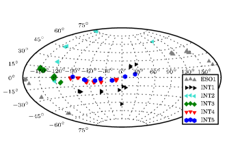
Figure 1: The position of the field centres of all the fields observed during the first five years of the RATS project. The fields are plotted in Galactic coordinates using an Aitoff projection. Many of the fields are spatially close and so appear as only a single point in this figure.

As during our first epoch of observations, we take a series of 30 second exposures of the same field for $\sim$2 hours. With a dead-time of $\sim$30 s for the INT observations and $\sim$110 s for the ESO/MPG 2.2-m fields, this results in approximately one observation every minute and every 2 minutes for the INT and ESO/MPG 2.2-m fields, respectively. To ensure the highest possible signal-to-noise we do not use a filter.

Before the white light sequence commences we observe the field in a number of filters. At earlier epochs we used Bessell B and V and either Bessell $I$ or SDSS $i^{\prime}$ filters whilst at later epochs we used RGO U and SDSS $g^{\prime}$ and $r^{\prime}$ filters, with the addition of a Heii 4686 Å narrow-band filter at the latest epoch (cf. Table 1). For the INT2 and ESO1 observations an autoguider was used, for the other epochs no autoguider was used.

The WFC on the INT consists of four $4096\times 2048$ pixel CCDs and has a total field of view of 0.28 square degrees. The four CCDs have a quantum efficiency which peak at 4600 Å and an efficiency above 50 per cent from 3500–8000 Å. The WFI on the MPG/ESO 2.2m has eight $4098\times 4046$ CCDs which are optimised for sensitivity in the blue and has a total field of view of 0.29 square degrees. We have observed a total of 110 fields which cover 31.3 square degrees of which 16.2 square degrees are at low galactic latitudes ($|b|<10^{\circ}$).

Images were bias subtracted and a flat-field was removed using twilight sky-images in the usual manner. In the case of our white light, $I$ and $i^{\prime}$ band images, fringing was present (in the absence of thin cloud). We removed this effect by dividing by a fringe-map made using blank fields observed during the course of the night.

Table 1: Summary of the six epochs in which our observations were taken. The number of stars column refers to sources with at least 60 photometric data points.

Epoch	Dates	# of	Galactic	Total	Filters
ID		fields	latitudes	stars
INT1	20031128-30	12	$>|16^{\circ}|$	45572	$BVi^{\prime}$
INT2	20050528-31	14	a	234029	$BVi^{\prime}$
ESO1	20050603-07	20	b	750109	$BVI$
INT3	20070612-20	26	$<|15^{\circ}|$	1223803	$Ug^{\prime}r^{\prime}$
INT4	20071013-20	29	$<|10^{\circ}|$	678025	$Ug^{\prime}r^{\prime}$
INT5	20081103-09	9	$<|10^{\circ}|$	112788	$Ug^{\prime}r^{\prime}$+Heii
a3 fields $<|10^{\circ}|$ and 11 fields $>|22^{\circ}|$
b4 fields $<|10^{\circ}|$ and 16 fields $>|16^{\circ}|$

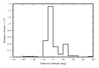
Figure 2: The galactic latitudes of all the stars observed during the first fiveyears of the RATS project that have more than 60 photometric data points. Our fields are biased towards the Galactic equator: 78 percent of the stars in our sample lie within $|b|<10^{\circ}$.

3 Photometry

3.1 Extracting light curves

In our first set of observations (Ramsay & Hakala, 2005) we used the Starlink aperture photometry package, Autophotom. This technique provides accurate photometry at a reasonable computational speed for fields with low stellar density, but proved to be unsuitable for fields containing more than a few 1000 stars due to the computational processing time involved and – for very crowded fields – its inability to separate blended stars.

For this reason we now use a modified version of Dandia (Bond et al., 2001; Bramich, 2008; Todd et al., 2005) – an implementation of difference image analysis (Alard & Lupton, 1998) – which is more suited to crowded fields and takes into account changes in seeing conditions over the course of the observation. The source detection threshold is set to $3\sigma$ above the background. We split each CCD into 8 sub-frames and calculated the point-spread function (PSF) for each sub-frame using stars that are a minimum of $14\sigma$ above the background and have no bad pixels nearby. A maximum of 22 stars are used in calculating the PSF. We use the four images with the best seeing in each field to create a reference frame. For each individual frame we degrade the reference frame to the PSF of that image and subtract the degraded reference frame. After subtraction we perform aperture photometry on the residuals. We do this for every frame and create a light curve for every star made up of positive and negative residuals.

As expected, our data suffer from systematic trends caused by effects such as changes in airmass and variation in seeing and transparency (for a discussion of systematic effects in wide-field surveys see Collier Cameron et al., 2006) which can cause the spurious detections of variable stars at specific periods. These periods are typically half the observation length, although they can occur at other periods and are field dependent. In order to minimise the effects of these trends we apply the Sysrem algorithm (Tamuz et al., 2005). The Sysrem algorithm assumes that systematic trends are correlated in a way analogous to colour-dependent atmospheric extinction, which is a function of airmass and the colour of each source. The colour is unique to each light curve and the airmass to each individual image though it does not necessarily refer to the true airmass but any linear systematic trend. These terms are minimised globally – and the trend removed – by modifying the measured brightness of each data point. We de-trend each CCD individually and use the method described in Tamuz et al. (2006) for running a variable number of cycles of the algorithm depending on the number of sources of systematic noise in the data, though we run a maximum of six cycles as we find that more than this starts to noticeably degrade signals in high-amplitude variables.

To determine the quality of the resulting light curves we calculated the root mean square (rms) from the mean for each light curve. When calculating the rms we sigma-clip each light curve at the $5\sigma$ level in order to remove the effects of, say, single spurious data points. In Fig. 3 the measured rms is shown as a function of the $g^{\prime}$ mag for all stars in our sample. The mean rms of all the data is 0.046 mag with sources brighter and fainter than $g^{\prime}=21.0$ having a mean rms of 0.024 and 0.051 mag, respectively. If we look at the mean rms of each field individually, we find two fields in our whole data-set with mean rms outside of 3 standard deviations which we attribute to very large variations in atmospheric transparency during these observations. We show the best-fitting exponential function to the expected rms (equivalent to the average error on each light curve) in Fig. 3 and find it to be consistent with the measured rms except of the very faintest stars ($g^{\prime}>22$).

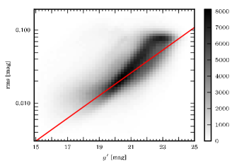
Figure 3: The rms noise of each light curve plotted against $g^{\prime}$ magnitude. The grey-scale refers to the number of sources in each bin. The red line is the best-fit exponential function to the expected rms – that is, the mean error of each light curve

3.2 Determining colours

When conditions appeared photometric we obtained images in different filters of a number of Landolt standard fields (Landolt, 1992). We made use of data kindly supplied by www.astro-wise.org who give the magnitude of Landolt stars in a range of different filters. We assumed the mean atmospheric extinction co-efficients for the appropriate observing site. The resulting zero-points were very similar to that expected.

For our target fields we initially used SExtractor (Bertin & Arnouts, 1996) to obtain the magnitude of each star in each filter. However, in comparison to Daophot (Stetson, 1987), SExtractor gave systematically fainter magnitudes for faint sources. Since the photometric zero-point for Daophot is derived from the PSF (and therefore different from field-to-field) we calculated an offset between the magnitudes of brighter stars determined using SExtractor and Daophot. We then applied this offset to the magnitudes derived using Daophot. To convert our $BVi^{\prime}$ data (Table 1) to $g^{\prime}r^{\prime}$ magnitudes we used the transformation equations of Jester et al. (2005).

Although our light curves were obtained in white light we note the depth of our observations as implied in the $g^{\prime}$ filter. For stars with $(g-r)\sim$1.0, the typical depth for fields observed in photometric conditions and with reasonable seeing (better than 1.2 arcsec) is $g\sim 22.8-23.0$, while for redder stars ($g-r\sim$2.0) the depth is $g\sim 23.6-24.0$.

To test the accuracy of our resulting photometry, we obtained a small number of images of SDSS fields (York et al., 2000). For stars $g^{\prime}<20$ we found that for $g_{\mathrm{RATS}}-g_{\mathrm{SDSS}}$, $\sigma$=0.12 mag and $(g_{\mathrm{RATS}}-r_{\mathrm{RATS}})-(g_{\mathrm{SDSS}}-r_{\mathrm{SDSS}})$, $\sigma$=0.22. For stars $20<g<22$ we find for $g_{\mathrm{RATS}}-g_{\mathrm{SDSS}}$, $\sigma$=0.29 mag and $(g_{RaTS}-r_{RATS})-(g_{\mathrm{SDSS}}-r_{\mathrm{SDSS}})$, $\sigma$=0.27. Given our project is not optimised to achieve especially accurate photometry these tests show that our photometric accuracy is sufficient for our purposes, namely determining an objects brightness and approximate colour.

3.3 Astrometry

As part of our pipeline we embedded sky co-ordinates into our images using software made available by Astrometry.net (Lang et al., 2010). This uses a cleaned version of the USNO-B catalogue (Barron et al., 2008) as a template for matching sources in the given field. The only input we provide is the scale for the detectors and the approximate position of the field, which is taken from the header information in the images. The Astrometry.net software works well in either sparsely or relatively dense fields. By comparing the resulting sky co-ordinates of stars with matching sources in the 2MASS (Jarrett et al., 2000) the typical error was 0.3–0.5 arcsec.

4 Variability

Due to the large data-set, it is necessary for us to automate the detection of variable sources. We find that no single algorithm is appropriate for the detection of all types of variable sources present in our data and in most cases for the detection of even a single class of variable source since the false positives are unacceptably high if we use just one algorithm. We therefore, typically use at least two independent algorithms to detect each class of variable object.

Before passing the light curve data to the variability detection algorithms we remove light curves which contain less than 60 data points. Of the initial 3.7 million stars, this leaves 3.0 million. We remove light curves with relatively few data points because our variability detection algorithms can produce spurious results when a significant amount of data are missing. This process prevents the discovery of transient phenomena, an aspect which we will investigate in more detail in the future.

In future work we will discuss sources such as contact and eclipsing binaries and flare stars whose variability is not periodic over a two hour time-frame. However, in this paper we will concentrate on the detection of periodic variables.

4.1 Periodic variability detection

We use two algorithms in order to identify variable sources: analysis of variance (AoV), and the Lomb-Scargle periodogram (LS). From these algorithms we determine the analysis of variance formal false-alarm probability, AoV-FAP; and the Lomb-Scargle formal false-alarm probability, LS-FAP. We use the Vartools suite of software to calculate these parameters (Hartman et al., 2008).

The Lomb-Scargle periodogram (Lomb, 1976; Scargle, 1982; Press & Rybicki, 1989; Press et al., 1992) is an algorithm designed to pick out periodic variables in unevenly sampled data. As a test of variability we use the LS-FAP. Its distribution as a function of magnitude is shown in Fig. 4. This parameter is a measure of the probability that the highest peak in the periodogram is due to random noise. If the noise in our data were frequency independent the LS-FAP would refer to the probability of the detected period being due to random noise. However, our data are subject to sources of systematic error which we attribute to red noise: these include the number of data points in the light curve and the range in airmass at which a star is observed. Hence, we use it as a relative measure of variability.

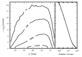
Figure 4: The distribution of the LS-FAP statistic in magnitude and number where the LS-FAP is for the highest peak in the frequency range. The contours refer to the number of stars in each bin where the data was been binned and has a bin size of 0.2 and 0.4 in magnitude and $\log(\textrm{LS-FAP})$, respectively.

We use a modified implementation of the analysis of variance periodogram (Schwarzenberg-Czerny, 1989; Devor, 2005). The AoV algorithm folds the light curve and selects the period which minimises the variances of a second-order polynomial in eight phase-bins. A periodic variable will have a small scatter around its intrinsic period and high scatter on all other periods. The statistic $\Theta_{AoV}$ is a measure of the goodness of the fit to the best fitting period, with larger values indicating a better fit. In order to be consistent with the LS-FAP we calculate the formal false-alarm probability of the detected period being due to random noise (AoV-FAP) – with the same caveats as with the LS-FAP – using the method described by Horne & Baliunas (1986). We show the distribution of the AoV-FAP statistic in number and as a function of magnitude in Fig. 5.

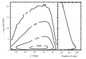
Figure 5: A similar plot to Fig. 4 but this time showing the distributions for AoV-FAP. The data is binned and the bin size is 0.2 and 0.4 in magnitude and $\log(\textrm{AoV-FAP})$, respectively.

The AoV algorithm, while similar to the LS method, should allow better variable detection as it fits a constant term to the data as opposed to subtracting from the mean as is done in the LS routine (Hartman et al., 2008). However we find that AoV has a number of negative features. It suffers from severe aliasing at periods of 2–3 min and for this reason we only search for periods longer than 4 min. In addition there is a tendency to detect a multiple of the true period when the true period is less than $\sim$40 min. In tests with simulated light curves we found approximately 10 per cent of sources with a period of 20 min were detected by AoV as having 40 min periods. The main weakness of the LS algorithm is that if a source has a periodic modulation in brightness for only a small amount of the total light curve then – according to the LS-FAP – it is detected as significantly variable. This leads to a large number of false-positive detections which are probably due to random noise. To combat this we have developed a technique to combine the AoV and LS algorithms.

Our technique, which combines the LS-FAP and AoV-FAP statistics is a multi-stage process. The first step is to determine if the source is detected as significantly variable by both the LS and AoV algorithms: we then test whether the period each algorithm detects is the same. Shown in Fig. 6 are the AoV-FAP and LS-FAP statistics plotted against the period that is measured by the respective methods. We can see here that both algorithms suffer from deficiencies: the distributions of AoV-FAP and LS-FAP are not constant with period, but tend to higher significance at longer periods. In order to account for the bias of the distribution we use an approach whereby we bin the data in period with each bin 2 min wide. A source passes the first two stages of the algorithm if it is above a specific significance in both AoV-FAP and LS-FAP relative to the other sources in the period bin. In order to determine this significance we use the median absolute deviation from the median (MAD, Hampel, 1974) which is defined for batch of parameters $\{x_{1},\ldots,x_{n}\}$ as

$$\mathrm{MAD}_{n}=b\>\mathrm{med}_{i}|x_{i}-\mathrm{med}_{j}x_{j}|$$ (1)

where $b$ is a constant which makes the parameter consistent with the standard deviation. For a Gaussian distribution $b=1.4826$ (Rousseeuw & Croux, 1993) which we use for simplicity. We use the median, as using the mean is not appropriate when the first moment of the distribution tail is large (Press et al., 1992); the large tails in the distributions of AoV-FAP and LS-FAP are shown in the right-hand plots in Figs. 4 and 5. The median and MAD are more robust statistics.

We vary the number of MADs a source must be above the median to be detected depending on epoch as the distributions of LS-FAP and AoV-FAP parameters are different. For INT2 and ESO1 we use 200 MADs, for INT1, INT4 and INT5 we use 800 MADs. These number of MADs above the median are used as they provide an appropriate balance between low amplitude detections and false positives – which we discuss in § 4.2 and § 4.3 – we attribute the need for different numbers of MAD above the median to the use of an autoguider on INT2 and ESO1 and not on the other epochs. Due to different epochs having different distributions of variability parameters we calculate the median independently for each epoch.

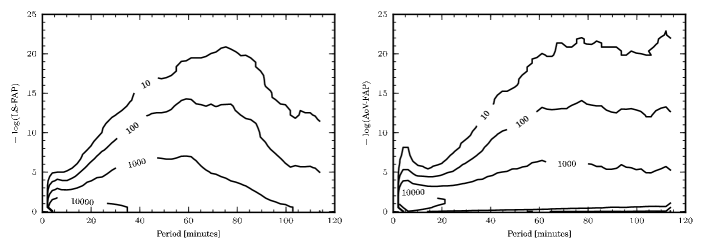
Figure 6: LS-FAP and AoV-FAP statistics in the left and right plots respectively, plotted against the period measured by those statistics. Spurious detections of variability are obvious at very short periods in AoV-FAP, while LS-FAP is less sensitive to longer period variability.

Both AoV and LS algorithms produce a periodogram; from the highest peak in the periodogram we calculate the most likely period of a given light curve. We take all the candidate variables and test whether the period detected by AoV matches that detected by LS. We class a period as a match if

$$P_{AoV}\pm\Delta P_{AoV}=P_{LS}\mp\Delta P_{LS}$$ (2)

where $P_{AoV}$ and $P_{LS}$ are periods detected by the two algorithms AoV and LS, respectively. $\Delta P$ is the error in measured period. We determine $\Delta P$ using an approximation of equation (25) in Schwarzenberg-Czerny (1991) whereby we assume that

$$\Delta P/P^{2}\sim k.$$ (3)

This assumption holds for all but the lowest signal-to-noise detection of variability. In order to determine an appropriate value for the constant, k, we inject sinusoidal signals of various periods into non-variable light curves and measure the standard deviation on $|P_{AoV}-P_{LS}|$. We set the constant, k, in Eq. 3 so as to give a $\Delta P$ at a given period equal to twice the standard deviation of $|P_{AoV}-P_{LS}|$. We find $k=0.002$ to be appropriate. The AoV algorithm has an annoying habit of detecting a multiple of the true period, so for this reason we modify Eq. 2 to

$$\frac{P_{AoV}}{n}\pm\Delta P_{AoV}=P_{LS}\mp\Delta P_{LS}$$ (4)

where $n=\{1,2,3,4\}$.

Sources that have matching periods and have been classified as candidate variable sources by both AoV-FAP and LS-FAP are then regarded as ’significantly’ variable sources. We detect 124334 stars which show variability on a timescale of 4–115 min: the distribution of the measured periods are shown in Fig. 7. We caution that this technique can detect variables that are not truly periodic – many flare stars have detected periods near the observation length – or may have periods longer than that detected by our method – contact binaries typically have a true period twice the measured one. If a period of less than half the observation length is measured then this is likely to be a true period. However, longer periods detected by the LS and AoV algorithms indicate only that the source varies significantly on time-scales less than $\sim$2 hours.

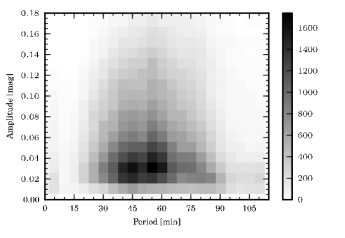
Figure 7: The amplitude and period of sources classes as variable using the technique for combining LS-FAP and AoV-FAP. The grey-scale uses bin size of 0.01 mag in amplitude and 5 min in period and the colour refers to the number of sources in that bin.

4.2 False positives

In order to determine the false positive detection rate, that is, the chance of a source with variability due to noise being identified as a real variable, we pick a light curve at random from the whole data set and construct a new light curve using a bootstrapping approach. The light curve consists of three columns of data: time, flux and error on the flux. We keep the time column as it is, and for a light curve with N individual photometric observations, randomly select N fluxes and errors from the N points in the original light curve. We do not limit the number of times a flux-error combination is selected. The reason for reconstructing a light curve in this fashion is that any periodic variability which is present in the original light curve is removed, allowing us to measure the chance that any variability present is due to noise.

We reconstruct $10^{5}$ bright and $10^{5}$ faint randomly selected light curves and attempt to detect variability using our method for combining the AoV and LS algorithms. Bright and faint refers to sources brighter than and fainter than $g^{\prime}=21.0$, respectively where 21.0 is approximately the median $g^{\prime}$ magnitude. For the bright sample we class 10 stars as variable and for the faint sample this increases to 17. This equates to a false positive rate of 0.01 and 0.02 per cent for bright and faint sources, respectively.

To find the improvement in the false positive detection rate we run the same routine but using only one of the statistics, i.e. LS-FAP or AoV-FAP. The method of detection is the same as the first stage of the two algorithm method – is a source found to have a variability statistic above the detection threshold for its period. When using both AoV-FAP and LS-FAP the false-positive rate is around 0.5 per cent. When using the two algorithm method the number of false positives is reduced by a factor of $\sim 40$.

4.3 Sensitivity tests as a function of amplitude and period

To determine the space densities for different classes of sources which vary on time-scales of less than $\sim$2 h it is essential that we determine our sensitivity to different brightnesses, periods and amplitudes. To do this we inject sinusoids of known period and amplitude into non-variable light curves and then attempt to detect it using our LS-FAP + AoV-FAP test. We split the sources into a bright and faint groups – brighter or fainter than $g^{\prime}=21.0$. – and for each brightness range we inject a periodic signal into a non-variable light curve. The non-variable light curve is drawn randomly from a pool of light curves that have AoV-FAP and LS-FAP statistics within 0.5 median absolute deviations of the median AoV-FAP and LS-FAP of all light curves with $g^{\prime}$ greater than and less than 21.0 for the bright and faint groups, respectively. The periodic signal injected is drawn from a grid of period-amplitude combinations where the periods range from $4-120$ min and amplitudes from $0.02-0.2$ mag. We define amplitude as peak-to-peak. The advantage of using real (non-variable) light curves over simulated data is that it preserves the noise values which may be non-Gaussian.

We run the entire grid 100 times for each brightness range which allows us to build up confidence of a variable with a given period and amplitude being detected. The results of this are plotted in Fig. 8 and show that in the brighter sample, sources with a period less than 90 min have a $\sim$70 per cent chance of being detected if they have amplitudes larger than 0.05 mag, rising to above a 90 per cent chance for amplitudes greater than $\sim 0.10$ mag. Stars fainter than $g^{\prime}=21.0$ with an injected period less than 90 min have $\sim$ 50 per cent detection chance if they have an amplitude greater than 0.08 mag and only sources with a period less than 40 min and an amplitude greater than $\sim$0.15 mag have a 90 per cent chance of detection.

From these results we find that our LS-FAP + AoV-FAP method is relatively good at identifying variables with periods less than 90 min in bright sources but is weaker at identifying periodic variability in the fainter sources. The advantage of this method is the small number of false-positives expected to be detected.

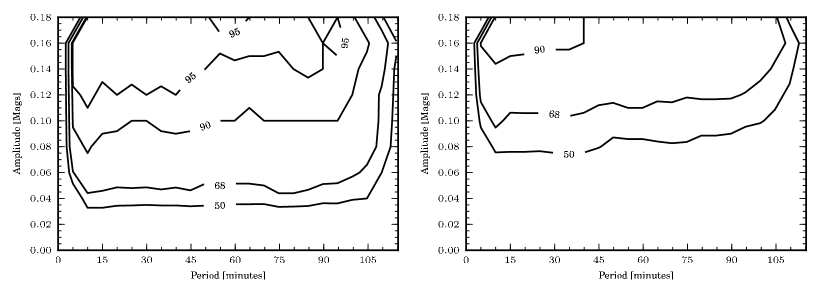
Figure 8: Our sensitivity to periodic sources of different period and peak-to-peak amplitudes. In the left plot, the contours refer to the percentage of sources detected as variable when the original non-variable light curve was brighter than $g^{\prime}=21.0$. The right plot show the same but for sources fainter than $g^{\prime}=21.0$.

4.4 Summary of variables in RATS

We have detected 124334 stars which show variability on timescales 4–115 min. This equates to 4.1 per cent of the total stars – with at least 60 data points – in our survey, of which 22679 sources have periods detected by the LS algorithm of less than 40 min. We expect 0.02 per cent – equal to $\sim$600 sources – of the variables detected in the RATS data to be false positives. The median value of the $g^{\prime}$ band magnitude is 21.0, whereas the median brightness of all variables is 21.5 and only 30 per cent of variables are brighter than the median brightness of all stars in the RATS data.

5 Colour of sources which vary on time-scales of less than two hours

We show the colours of all the stars in our data in the $g^{\prime}-r^{\prime},g^{\prime}$ plane in left hand panel of Fig. 9. We note the presence of two broad populations; one which is bright ($g^{\prime}\sim 19-21$) and blue ($g^{\prime}-r^{\prime}\sim 0.6-0.7$), and one which is fainter ($g^{\prime}\sim 22-23$) and redder ($g^{\prime}-r^{\prime}\sim 1.5-2.0$). The bluer population is thought to originate in the Galactic halo or thick disk, while the redder population is thought to originate in the thin disk (e.g. Robin et al., 2003). Data similar to these has been used to model the structure of the Milky Way as a function of Galactic latitude and longitude (cf. Chen et al., 2001), but this is beyond the scope of the present work.

We also show in Figure 9 the stars which have been classified as variable (cf. §4) in the $g^{\prime}-r^{\prime},g^{\prime}$ plane. The variable sources are concentrated at the faint, red end of the of the colour-magnitude diagram. In contrast, the Faint Sky Variability Survey (FSVS) found that the variable sources they detected were biased towards bluer colours (Morales-Rueda et al., 2006). We attribute this difference to the fact that the FSVS was more typically sensitive to longer time-scale variations than our survey, coupled with the fact that they observed fields at mid to high Galactic latitudes (Groot et al., 2003).

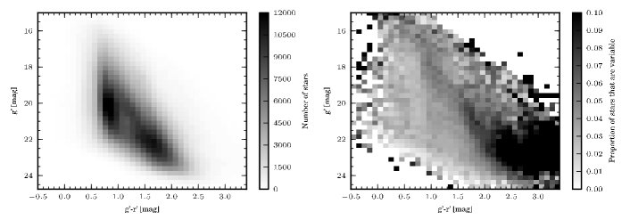
Figure 9: Colour-magnitude diagram showing $g^{\prime}-r^{\prime}$ against $g^{\prime}$ magnitude. The left plot contains all the stars in our data, the right plot show the proportion of stars in each bin that are classified as variable using the method in §4.3.

6 Short period blue variables

AM CVn systems show optical modulation on a period close to their orbital period and are intrinsically blue in colour – the reddest have $g^{\prime}-r^{\prime}$ colours of $-0.1$ – and modulate on periods of $<40$ min with amplitudes from 0.01–0.30 mag. In this section we restrict our search to stars with parameters fulfilling these criteria.

The known AM CVn systems found in SDSS data have de-reddened $g^{\prime}-r^{\prime}<-0.1$ (Roelofs et al., 2009). The majority of our stars are close to the Galactic plane where the interstellar reddening is high. For fields close to the Galactic plane ($|b|<15^{\circ}$) we adopt an average value for the total neutral hydrogen column density to the edge of the Galaxy of $N_{H}=3.67\times 10^{21}$ cm^-2 which is taken from the Leiden/Argentine/Bonn (LAB) Survey of Galactic HI (Kalberla et al., 2005). We calculate the optical extinction in the $V$ band, $A_{V}$ using the relation found by Güver & Özel (2009):

$$N_{H}=(2.21\pm 0.09)\times 10^{21}A_{V}.$$ (5)

We take $A_{V}=3.10\times E(B-V)$ (Fitzpatrick, 1999) which gives $A_{V}=1.66$ and $E(B-V)=0.54$. This result is consistent with Joshi (2005) who observed open clusters close to the Galactic plane ($|b|<5^{\circ}$) and find $E(B-V)=0.6$. If we convert this extinction calculated from the $N_{H}$ of our fields to Sloan $g^{\prime}$ and $r^{\prime}$ filters we find $E(g^{\prime}-r^{\prime})=0.60$. Adding this to the red cutoff for AM CVn systems $(g^{\prime}-r^{\prime}<-0.1)$ we get a cutoff of for AM CVn systems in our data which are close to the Galactic plane, of $g^{\prime}-r^{\prime}<0.5$

After these cuts the number of sources left as candidate AM CVn systems is 250. We visually inspect these as a final level of quality control, and class 66 of these short-period blue variables as ‘good’ candidates – that is, having a strong period and no obvious systematic effects present.

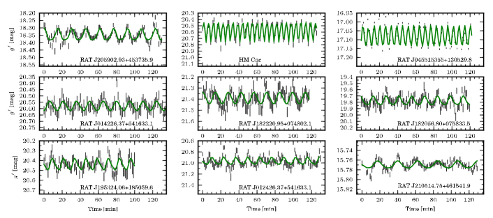
Figure 11: A sample of the blue short-period variable stars shown in Table 2. The green curve shows the best-fitting amplitude, period and phase of the light curve. The period was found using the Lomb-Scargle periodogram algorithm, the amplitude and phase from fitting a sine curve to the light curve on that period.

In Tabs. 2 and 3 we list the short period blue variables for those sources with periods less than 25 min and for those with periods 25–40 min, respectively. We split these into two tables for ease of comparison with Nelemans et al. (2001, 2004) model of the Galactic population of AM CVn systems which is only relevant for sources with periods less than 25 min (see § 8). The sources contained in these two tables are plotted as blue dots in Fig. 10. A subset of the light curves of these sources are shown in Fig. 11. We fit a sinusoid to each light curve at the period of the highest peak in the Lomb-Scargle periodogram and this is shown over-plotted on each light curve.

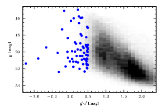
Figure 10: Colour-magnitude diagram of all the detected variable stars plotted as grey-scale. Those stars identified as short period ($P<40$ min) blue variables – shown in Table 2 and 3 – are shown as blue dots.

Table 2: Sources identified as periodic variable stars with periods less than 25 min and a $g^{\prime}-r^{\prime}$ colour of less than 0.5. They have also passed a visual quality check. The period is determined from the Lomb-Scargle periodogram and the amplitude is peak-to-peak of the best fitting sine curve. If classification of the source has been possible then this is stated in the notes column. For the previously know sources the classification come from the literature, for the newly discovered variables we classify the sources based on spectral type and the spectral fitting described in § 7.2. The Cat. name column is the unique identifier for that source and is of the format EpochID-Field#-CCD#-Star#.

Cat. name	R.A. (J2000)	Dec. (J2000)	Period [min]	$g^{\prime}$ [mag]	$g^{\prime}-r^{\prime}$ [mag]	Amplitude [mag]	Notes	Ref.
4-7-3-9108	01:41:31.42	+55:34:11.3	5.31	20.48	0.18	0.033		3
4-11-1-2519	01:42:26.37	+54:16:33.1	13.23	21.12	$-$0.00	0.128	1	3
5-6-3-4828	04:32:10.40	+40:33:33.9	8.43	20.10	$-$0.34	0.249	1	3
1-16-4-1316	04:55:15.22	+13:05:29.8	6.24	17.32	$-$0.22	0.115	Pulsating sdB star	4
4-27-3-662	05:07:51.28	+34:31:55.5	22.15	16.31	0.03	0.029	2	3
1-22-4-1415	07:39:19.05	+23:52:39.9	14.71	20.83	0.06	0.074	1	1
1-806-4-713	08:06:22.95	+15:27:31.2	5.36	20.77	$-$0.89	0.284	AM CVn star	5
3-2-3-14617	17:58:46.34	+01:45:59.8	9.58	22.00	0.26	0.103		3
3-5-1-25551	17:59:52.90	+01:22:19.4	22.10	20.01	0.49	0.028		3
3-5-3-4143	18:00:57.72	+01:42:03.0	20.40	20.48	0.34	0.038		3
2-7-2-1301	18:01:52.91	+29:42:30.4	8.55	19.92	0.06	0.058		3
3-26-1-604	18:20:56.80	+07:58:33.5	14.20	19.96	0.14	0.134		3
3-27-2-6182	18:22:20.95	+07:48:02.1	14.17	21.24	0.22	0.103	1	3
2-11-4-34562	19:53:24.03	+18:50:59.6	12.38	20.68	$-$0.06	0.109		3
2-11-3-25021	19:53:27.17	+18:59:14.4	20.00	19.98	$-$0.07	0.240	Dwarf nova	6
4-9-2-9694	20:58:00.24	+45:32:32.8	7.23	19.16	0.50	0.039		3
4-9-4-14918	20:59:02.93	+45:37:35.9	15.34	18.36	$-$0.06	0.080	Pulsating white dwarf	3
4-16-4-21281	21:05:14.75	+46:15:41.9	22.42	15.77	0.25	0.014	2	3
1-3-2-46	23:03:11.95	+34:31:04.1	9.20	20.78	0.47	0.040		3
4-6-4-2813	23:49:06.89	+56:24:40.4	22.73	18.06	0.32	0.039	2	3
4-6-3-470	23:49:29.00	+56:34:26.2	5.82	16.58	0.25	0.018		3
4-25-3-9719	23:52:42.07	+56:31:53.2	12.85	19.46	$-$0.66	0.098		3
1Low signal-to-noise spectrum – no obvious emission lines,2A-type star spectrum
3This paper, 4Ramsay et al. (2006), 5Ramsay et al. (2002), 6Ramsay et al. (2009)

Table 3: The same as Table 2 for sources with periods between 25 and 40 min.

Cat. name	R.A. (J2000)	Dec. (J2000)	Period [min]	$g^{\prime}$ [mag]	$g^{\prime}-r^{\prime}$ [mag]	Amplitude [mag]	Notes	Ref.
5-7-2-1129	06:54:32.71	+10:31:52.8	35.92	16.00	0.10	0.032		3
5-7-4-9019	06:55:15.30	+10:38:59.0	33.87	15.92	0.34	0.015	2	3
5-7-4-7787	06:55:26.31	+10:36:48.4	39.19	15.96	0.30	0.013		3
5-7-4-7234	06:55:31.08	+10:35:31.8	30.67	17.13	0.49	0.015		3
5-7-4-3601	06:56:04.22	+10:34:35.3	28.62	17.01	0.48	0.021		3
5-7-3-1149	06:56:33.59	+10:45:41.4	33.87	19.02	0.17	0.036	1	3
3-8-1-21492	17:54:29.79	+01:37:52.2	29.77	21.38	$-$1.23	0.057		3
3-5-3-16324	17:59:58.53	+01:50:28.5	38.63	19.46	0.49	0.020		3
3-14-2-12275	18:00:02.54	+00:34:08.4	34.76	19.53	0.38	0.034		3
3-14-3-6993	18:01:06.36	+00:54:18.1	36.91	21.16	0.17	0.097		3
3-5-3-1384	18:01:11.05	+01:46:36.4	38.39	21.39	0.46	0.085		3
3-11-2-3507	18:02:50.62	+00:43:52.8	34.14	18.97	0.29	0.048		3
3-11-3-14721	18:03:18.71	+00:57:30.1	28.61	21.88	0.47	0.092		3
3-11-3-14333	18:03:20.82	+00:52:40.9	33.09	20.91	0.43	0.053		3
3-11-3-14041	18:03:22.48	+00:52:07.8	33.73	21.11	0.46	0.047		3
3-11-3-176	18:04:45.09	+00:53:26.4	37.53	21.72	$-$0.12	0.148		3
3-24-3-21598	18:16:48.03	+06:16:11.4	39.49	21.54	0.50	0.121		3
3-24-3-27252	18:17:41.11	+06:39:30.2	33.88	21.95	0.48	0.144		3
3-24-3-27068	18:17:41.80	+06:39:55.2	33.88	19.17	0.47	0.019		3
3-24-3-26839	18:17:42.61	+06:39:47.5	37.50	20.11	0.39	0.031		3
3-24-3-25379	18:17:47.71	+06:42:21.7	37.62	19.63	0.50	0.022		3
3-24-3-24553	18:17:50.35	+06:40:36.7	38.22	19.37	0.36	0.027		3
3-24-4-10602	18:17:52.98	+06:31:33.2	37.04	21.55	0.47	0.084		3
3-24-3-23361	18:17:54.38	+06:41:38.7	38.22	20.92	0.33	0.074		3
3-24-3-22275	18:17:58.05	+06:42:55.7	38.97	19.86	0.48	0.026		3
3-24-3-20681	18:18:03.13	+06:39:50.2	25.16	19.78	0.30	0.024		3
3-24-4-7636	18:18:12.79	+06:26:23.7	29.67	22.38	$-$0.31	0.107		3
3-24-3-13813	18:18:26.67	+06:44:01.8	37.62	21.45	0.36	0.067		3
3-24-3-13658	18:18:27.31	+06:47:06.2	36.70	19.33	0.46	0.024		3
3-24-1-8755	18:18:32.46	+06:23:19.9	35.92	19.41	0.48	0.021		3
3-24-3-11788	18:18:33.04	+06:37:17.9	39.49	18.25	0.45	0.024		3
3-24-3-11343	18:18:34.46	+06:37:09.7	34.97	20.85	0.48	0.048		3
3-24-3-11006	18:18:35.62	+06:38:43.4	35.08	21.44	0.46	0.074		3
3-17-2-5279	18:21:41.24	+08:22:28.3	27.85	19.70	0.21	0.041		3
3-27-1-24759	18:23:14.11	+07:36:50.9	34.05	20.48	0.28	0.049		3
3-27-3-9867	18:23:36.70	+07:58:00.5	29.74	19.17	0.44	0.022		3
3-27-3-9744	18:23:37.56	+07:59:07.1	28.86	22.32	0.41	0.131		3
3-25-3-11740	18:42:54.64	+00:21:48.7	36.12	21.76	0.09	0.168		3
2-11-4-41975	19:53:06.30	+18:48:39.4	32.19	17.87	0.30	0.023	2	3
2-11-1-24882	19:53:35.94	+18:38:08.7	25.46	18.86	0.14	0.034	1	3
2-3-4-4027	20:02:18.77	+18:49:37.9	34.40	20.41	0.50	0.107		3
4-16-3-16761	21:05:03.14	+46:27:45.5	32.97	15.11	$-$0.16	0.034	2	3
4-16-4-21946	21:05:12.19	+46:20:38.3	31.82	14.98	0.22	0.022	2	3
4-6-4-11525	23:47:46.82	+56:28:52.0	31.34	21.15	0.09	0.094		3
1Low signal-to-noise spectrum – no obvious emission lines,2A-type star spectrum
3This paper

We searched for the 66 variables in Table 2 and 3 in the Simbad database and found three matches with 5 arcsec of our target. One is HM Cnc, an AM CVn system (Ramsay et al., 2002) and two are previously published sources which we found in the RATS data: a high amplitude pulsating subdwarf B star (Ramsay et al., 2006) which is a rare hybrid object as it exhibits both gravity and pressure modes of pulsation (Baran et al., 2010); and a dwarf nova with high amplitude quasi-periodic oscillations in quiescence (Ramsay et al., 2009). Of the other sources; 22 have periods less than 25 min, of which 9 have a period of less than 10 min. The amplitudes of the short-period blue sources ranges from 0.012–0.284 mag with a mean of 0.066 mag and the $g^{\prime}$ band brightness range from 14.9–22.4 mag with a mean of 19.6 mag.

7 Spectra of variable sources

7.1 Observations

We have a programme to obtain optical spectroscopic observations of variable sources found in our survey (cf. §4). These data are low resolution spectra with which to determine the nature of sources. Most data were obtained with the 4.2-m William Herschel Telescope on La Palma using the dual-beam ISIS instrument and the R300B and R158R gratings giving a wavelength coverage from 3500–10000Å.

Typically the slit-width was 0.8 arcsec and based on the FWHM of arc lines we estimate the spectral resolution to be approximately 3 and 6Å, for the blue and red spectra, respectively. Wavelength calibration was determined using Cu-Ar and Cu-Ne arc-lamps.

We have also used the ALFOSC instrument on the Nordic Optical Telescope for brighter targets and GMOS on the Gemini South telescope for the very faintest targets ($g^{\prime}>20$). Southern sources have been observed with EFOSC2 on the ESO 3.6m telescope at La Silla Observatory, Chile and the Grating Spectrograph on the 1.9-m Radcliffe telescope at the South African Astronomical Observatory.

We reduced these data using standard techniques and employ the packages Molly, Pamela and Starlink packages Figaro and Kappa. We used optimal extraction (Horne & Baliunas, 1986) and did not observe flux standards so normalised spectra by fitting a spline to the continuum. Arc lamp exposures were typically taken at the beginning, middle and end of each night and we calibrated each spectrum by interpolating between the arcs.

7.2 Fits with model spectra

The spectra we obtain are primarily for identification purposes (e.g. is the variable star a main sequence star or a hydrogen-rich white dwarf). However, for those cases where we have reasonable signal to noise we are able to determine a number of properties of the star through spectral fitting.

In order to determine surface temperatures, surface gravity and metallicities we fit the spectra we have obtained with model atmospheres using the Fits2b fitting programme (Napiwotzki et al., 2004). For stars with DA white dwarf spectra we fit the Balmer lines using a grid of hot white dwarf models (Koester et al., 2001) with temperatures ranging from 6000–100000 K and log g from 5.5–9.5. For all other spectra we use ATLAS9 model atmospheres (Castelli & Kurucz, 2004).

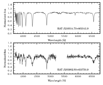
Figure 12: Two optical spectra made using the ISIS spectrograph on the WHT. The upper spectrum is of a pulsating A star with a 22.4 min period in its light curve. The lower plot is of a pulsating DA white dwarf which has an optical modulation present in the light curve on a period of 15.3 min.

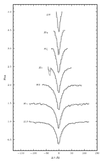
Figure 13: The Balmer lines of RAT J210514.75+461541.9 over-plotted by the best-fitting model. The continuum of has been normalised to unity and each line after $H\beta$ has been shifted up by 0.5 in flux. The best-fitting effective temperature and surface gravity are $8760\pm 80$ K and $4.15\pm 0.05$ dex, respectively.

We have WHT spectra of 12 of the newly discovered short-period blue variables. The classification which we have given individual sources as a result of this spectral fitting are shown in Table 2 and 3. One of these is a pulsating white dwarf which appears to be a composite of a WD pulsator of type DAV and a hotter companion (Barclay et al., in prep.), and 8 are sources with the spectral type of a main sequence A-type star. In Fig. 12 we show the normalised spectrum of the pulsating white dwarf and of one of the variable A-type stars. The Balmer lines ($H\beta$–$H\theta$) of this A-type star, RAT J210514.75+461541.9, are shown in Fig. 13. Over-plotted is the best-fitting ATLAS9 model, which has an effective temperature of $8760\pm 80$ K and a surface gravity of $4.15\pm 0.05$ dex, where the errors were determined using a bootstrapping technique. We used a model with solar metallicity. These parameters are fairly typical for an A-type star. The nature of this, and the other 7 A-type variables, is unclear. One possibility is that they are long period examples of rapidly oscillating, chemically peculiar A (roAp) stars which have typical pulsation periods of 10 min (e.g. Kochukhov et al., 2009) although longer periods – up to 21 min – have been seen (Elkin et al., 2005). Alternatively they could be low amplitude delta Scuti stars with a pulsation period at the very short period end of the delta Scuti period distribution. We are planning medium-high resolution spectroscopic observation in order to distinguish between there two scenarios: roAp stars show evidence of a marked overabundances of heavy elements in their spectra, whereas the delta Scuti stars show abundances similar to the Sun.

8 Space density of AM CVn systems

The combined sky coverage of the first 5 years of data is 31.3 square degrees. Nelemans et al. (2001, 2004) predict the space density of AM CVn systems with orbital periods less than 25 min as a function of Galactic latitude. This is done for a limit of $V<20$ and $V<22$ (for $B-V=0.2$, $V=g^{\prime}$). For the distribution of our fields these models predict 2.7 and 8.2 AM CVn systems with $P_{orb}<25$ min for $g^{\prime}<20$ and $g^{\prime}<22$, respectively.

In our survey we have identified 12 candidate AM CVn systems brighter than $g^{\prime}=20$ and 33 brighter than $g^{\prime}=22$ (cf. Table 2). We have obtained optical spectra of 23 candidates, none of these spectra are consistent with the source being an AM CVn system. Removing these sources leaves us with ten candidates AM CVn systems for which we are yet to obtain spectra that are brighter than $g^{\prime}=22$ of which six candidates are brighter than $g^{\prime}=20$. One could speculate that the observed sample, once follow-up is completed, will indicate the need to revise the simulations, but for the time being we are left with an upper limit of ten, which is consistent with the model of Nelemans et al. (2001, 2004).

In contrast, the work of Roelofs et al. (2007) suggests that based on the number of systems discovered in the SDSS data, the model of Nelemans et al. over-predicts the number of long period systems ($P_{orb}<25$ min) by a factor $\ga 10$. If this were to be replicated at shorter periods we would expect to find $<1$ AM CVn systems in our observations so far. It remains to be seen whether there is also a deficit of systems compared to the models at shorter periods, or whether there are relatively many more younger, short period systems compared with older systems. This is particularly important for future low-frequency gravitational wave detectors such as LISA.

9 Conclusions

Over the last decade, many surveys have set out to identify variable objects in specific stellar clusters or nearby galaxies, or over significant fractions of the sky, for instance in the search for transiting exo-planets. However, very few of these surveys have been able to identify sources with periodic variability on timescales as short as a handful of minutes and in the range $15\leq g\leq 22$. This brightness range is important as the number of stars in this range is vastly greater than at comparable brighter intervals, while still being suitable for follow-up spectroscopy.

We have found that in a survey such as RATS it is essential that potential sources of systematic variability are explored in detail. Further, if resources permit, a number of pilot studies would result in reducing the significance of these systematic effects. However, once these issues have been dealt with, we have found that RATS is very well suited to the discovery of variable stars with periods as short as 5 min or show flares (or eclipses) as short as 5–10 min. Further, we can also identify stars with periods up to an hour and stars which show variability over time-scales of several hours. Many of these sources are emerging as astrophysically interesting. However, the sheer number of variable sources will prevent us from following-up all the potentially interesting sources. For this reason we intend to release to the community the data products of the variable and non-variable sources presented in this paper by the second half of 2011.

The inspiration for this project was to identify new ultra-compact binaries. At this stage the implied space density of these objects is consistent with the predictions of Nelemans et al. (2001, 2004). However, we will not be in a position to make a definitive conclusion regarding this question until we have fully analysed the final 16 square degrees of data and obtained the essential follow-up spectroscopy of candidate systems. It remains to be seen as to whether a study like this is the optimum in identifying objects which appear to be intrinsically rare.

Appendix A Fields Observed

Table 4: Summary of the fields observed in the first 6 epochs of our survey. Field ID is in the format epoch-field#, see table 1 for a summary of each epoch. Field centre refers to the centre of CCD4 in the INT WFC observations and close to the centre in the case of ESO WFC observations. The duration is the time-span for the series of 30 sec exposures. The seeing was determined from the FWHM of the images; the number of light curves is those stars for which more than 60 data points were obtained.

Field ID	Date	RA DEC	$l,b$	Duration	Seeing	Number of
		(J2000)	(J2000)		(′′)	lightcurves
INT1-2	2003-11-28	22:57:08.9 +34:13:02	97.5 $-$22.9	2h 33m	0.8–1.3	4061
INT1-6	2003-11-28	02:08:10.7 +36:16:13	139.8 $-$24.1	2h 23m	1.0–1.5	2786
INT1-11	2003-11-28	04:11:31.1 +19:24:55	174.6 $-$22.8	2h 04m	1.0–1.5	2762
INT1-21	2003-11-28	07:29:20.0 +23:25:36	195.4 +18.4	2h 31m	1.0–1.5	4097
INT1-1	2003-11-29	23:10:43.9 +34:19:48	100.3 $-$24.1	2h 47m	1.2–2.0	3464
INT1-8	2003-11-29	02:02:15.6 +34:21:40	139.2 $-$26.3	2h 22m	1.3–2.6	3321
INT1-16	2003-11-29	04:55:55.5 +13:04:42	186.9 $-$18.4	2h 02m	0.9–1.3	4783
INT1-806	2003-11-29	08:06:23.0 +15:27:31	206.9 +23.4	2h 06m	0.8–1.1	4518
INT1-3	2003-11-30	23:04:48.0 +34:26:19	99.1 $-$23.4	2h 18m	0.7–1.1	4576
INT1-307	2003-11-30	03:06:07.2 $-$00:31:14	179.1 $-$48.1	1h 59m	1.0–1.4	1722
INT1-17	2003-11-30	04:50:42.5 +18:11:59	181.8 $-$16.4	2h 30m	0.9–1.3	4838
INT1-22	2003-11-30	07:39 51.9 +23:50:03	196.0 +20.8	2h 41m	0.9–1.3	4644
INT2-1	2005-05-28	13:57:08.6 +22:48:16	20.3 +74.5	1h 53m	1.5–3.0	988
INT2-2	2005-05-28	16:05:45.8 +25:51:45	42.8 +46.8	1h 53m	0.8–1.2	2209
INT2-3	2005-05-28	20:01:53.9 +18:47:41	57.8 $-$6.2	1h 57m	1.5–1.9	32428
INT2-4	2005-05-29	12:00:00.0 $-$00:00:00	276.3 +60.2	0h 56m	0.7–1.2	1517
INT2-5	2005-05-29	13:59:31.7 +22:10:56	18.9 +73.8	1h 51m	0.8–1.3	1590
INT2-6	2005-05-29	16:09:10.0 +24:00:13	40.4 +45.6	1h 51m	0.7–1.0	2634
INT2-7	2005-05-29	18:03:29.9 +29:56:25	56.1 +22.8	2h 09m	0.8–1.0	4333
INT2-8	2005-05-30	14:00:37.2 +22:45:59	21.2 +73.7	1h 57m	0.7–0.9	2511
INT2-10	2005-05-30	17:59:12.6 +28:25:20	54.2 +23.2	1h 51m	0.6–0.8	8465
INT2-11	2005-05-30	19:53:46.1 +18:46:42	56.7 $-$4.6	1h 40m	1.4–1.5	90451
INT2-12	2005-05-31	13:58:40.1 +23:34:19	23.5 +74.4	2h 26m	0.6–0.8	1983
INT2-13	2005-05-31	17:56:28.9 +29:09:39	54.7 +24.0	2h 02m	1.3–1.5	8172
INT2-14	2005-05-31	19:55:30.5 +18:42:04	56.9 $-$5.0	1h 57m	1.3–1.5	76748
ESO-1	2005-06-03	12:04:20 $-$24:50:31	289.6 +36.8	1h 46m	1.0–1.3	1573
ESO-2	2005-06-03	14:03:32 $-$22:17:05	324.1 +37.6	1h 56m	0.8–1.1	2872
ESO-5	2005-06-03	20:04:50 $-$24:04:46	17.9 $-$26.2	2h 32m	0.8–1.2	8000
ESO-4	2005-06-03	16:23:36 $-$26:31:39	351.0 +16.0	3h 28m	0.7–1.0	36424
ESO-7	2005-06-04	12:08:15 $-$22:56:35	290.1 +38.9	2h 37m	1.4–2.6	1356
ESO-8	2005-06-04	13:53:46 $-$23:41:48	320.9 +37.0	2h 25m	1.2–2.4	2567
ESO-10	2005-06-04	18:01:03 $-$26:54:22	3.5 $-$1.9	2h 16m	0.7–1.2	142523
ESO-13	2005-06-05	12:02:40 $-$22:32:40	288.4 +38.9	2h 28m	0.6–1.4	1696
ESO-14	2005-06-05	14:03:47 $-$24:55:05	323.1 +35.1	2h 27m	0.7–1.1	4402
ESO-16	2005-06-05	18:07:54 $-$24:56:23	5.9 $-$2.3	2h 32m	0.7–1.4	173696
ESO-17	2005-06-05	20:05:13 $-$22:32:36	19.6 $-$25.8	2h 35m	0.8–1.4	8711
ESO-19	2005-06-06	12:01:38 $-$24:25:27	288.7 +37.1	2h 28m	0.8–1.4	2556
ESO-21	2005-06-06	16:00:16 $-$25:33:01	347.9 +20.4	2h 27m	0.6–0.9	9877
ESO-22	2005-06-06	18:36:26 $-$23:55:04	9.9 $-$7.6	2h 32m	0.7–1.0	162417
ESO-6540	2005-06-07	18:06:01 $-$27:44:40	3.3 $-$3.3	2h 25m	0.6–0.8	185173
ESO-25	2005-06-07	12:08:07 $-$25:14:10	290.7 +36.6	1h 52m	0.6–2.0	3512
ESO-30	2005-06-07	22:03:11 $-$24:43:56	26.8 $-$52.3	2h 00m	0.6–0.9	2754

Field ID	Date	RA DEC	$l,b$	Duration	Seeing	Number of
		(J2000)	(J2000)		(′′)	lightcurves
INT3-2	2007-06-12	17:59:00 +01:38:00	28.4 +12.4	1h 45m	1.1–1.4	34275
INT3-3	2007-06-12	19:42:00 +19:06:00	55.6 $-$2.0	1h 19m	1.0–1.3	117341
INT3-4	2007-06-13	18:04:00 +02:20:00	29.6 +11.6	2h 08m	1.1-1.7	13194
INT3-5	2007-06-13	18:00:30 +01:35:00	28.5 +12.0	2h 00m	0.9–1.2	43524
INT3-6	2007-06-13	19:41:00 +19:48:00	56.1 $-$1.4	1h 53m	0.8–1.1	135686
INT3-7	2007-06-14	18:04:00 +01:31:00	28.8 +11.2	2h 05m	0.9–1.5	17583
INT3-8	2007-06-14	17:55:00 +01:46:00	28.0 +13.4	2h 00m	0.8–1.2	34249
INT3-9	2007-06-14	19:37:00 +19:47:00	55.6 $-$0.6	2h 00m	0.8–1.0	117956
INT3-10	2007-06-15	18:00:00 +02:13:00	29.0 +12.4	2h 16m	1.3–2.6	10358
INT3-11	2007-06-15	18:04:00 +00:46:00	28.2 +10.9	2h 20m	1.0–1.4	43084
INT3-12	2007-06-15	19:40:00 +22:50:00	58.6 +0.3	2h 00m	0.8–1.1	41726
INT3-13	2007-06-16	17:55:00 +02:22:00	28.5 +13.6	2h 06m	1.3–1.8	10323
INT3-14	2007-06-16	18:01:00 +00:42:00	27.7 +11.5	2h 00m	1.2–1.5	38365
INT3-15	2007-06-16	19:31:00 +19:03:00	54.3 +0.2	2h 04m	1.1–1.5	84418
INT3-16	2007-06-17	18:23:04 +05:53:25	35.0 +9.0	2h 17m	1.3–2.0	9553
INT3-17	2007-06-17	18:22:51 +08:25:34	37.3 +10.3	2h 10m	0.9–1.2	51788
INT3-18	2007-06-17	19:27:00 +22:40:00	57.0 +2.8	2h 09m	0.9–1.0	93095
INT3-20	2007-06-18	18:19:42 +05:52:01	34.6 +9.7	2h 04m	1.9–3.0	4622
INT3-21	2007-06-18	18:18:00 +07:35:41	36.0 +10.9	2h 00m	1.4–2.6	30470
INT3-22	2007-06-18	19:39:00 +20:24:00	56.4 $-$0.7	2h 00m	1.1–1.4	78067
INT3-24	2007-06-19	18:18:18 +06:31:15	35.0 +10.3	2h 00m	1.1–1.5	48472
INT3-25	2007-06-19	20:32:00 +25:11:00	67.0 $-$8.5	2h 00m	1.2–1.7	52974
INT3-26	2007-06-20	18:20:21 +08:11:47	36.8 +10.6	2h 00m	1.0–1.6	13554
INT3-27	2007-06-20	18:23:47 +07:51:23	36.8 +9.7	2h 00m	0.9–1.2	59027
INT3-28	2007-06-20	20:31:00 +27:26:00	68.7 $-$7.0	2h 00m	0.8–1.1	40099
INT4-1	2007-10-13	21:04:25.9 +45:40:34	87.2 $-$0.8	2h 16m	1.2–1.6	52237
INT4-2	2007-10-13	21:57:14.8 +54:01:00	99.1 $-$0.6	1h 56m	1.3–1.7	33917
INT4-3	2007-10-13	01:27:01.0 +53:50:51	128.2 $-$8.7	2h 09m	1.2–1.8	9355
INT4-4	2007-10-13	02:52:26.6 +50:42:29	141.7 $-$7.7	2h 55m	1.1–2.0	5707
INT4-5	2007-10-14	21:01:15.0 +44:30:47	85.9 $-$1.2	2h 20m	0.8–1.1	51566
INT4-6	2007-10-14	23:48:10.0 +56:26:08	114.2 $-$5.4	2h 29m	0.9–1.1	22154
INT4-7	2007-10-14	01:42:15.0 +55:21:46	130.2 $-$6.8	2h 10m	0.9–1.3	16942
INT4-8	2007-10-14	04:55:19.0 +34:42:02	169.2 $-$5.5	2h 19m	0.9–1.2	9030
INT4-9	2007-10-15	20:59:15.0 +45:34:42	86.5 $-$0.2	2h 21m	1.0–1.3	57117
INT4-10	2007-10-15	23:48:04.0 +54:19:49	113.7 $-$7.4	2h 19m	1.1–1.3	17730
INT4-11	2007-10-15	01:41:42.0 +54:33:14	130.2 $-$7.6	2h 10m	1.0–1.2	15605
INT4-12	2007-10-15	05:03:31.0 +34:56:22	170.0 $-$4.0	2h 16m	0.9–1.2	12597
INT4-13	2007-10-16	21:08:06.0 +44:14:06	86.5 $-$2.3	2h 10m	1.2–1.4	37264
INT4-14	2007-10-16	23:48:04.0 +54:19:49	113.7 $-$7.4	2h 00m	1.1–1.4	11212
INT4-16	2007-10-17	21:05:39.0 +46:20:27	87.8 $-$0.6	2h 10m	1.3–1.7	56719
INT4-17	2007-10-17	01:26:19.0 +54:49:00	128.0 $-$7.7	1h 54m	0.9–1.1	12945
INT4-19	2007-10-17	05:04:51.0 +36:14:33	169.1 $-$3.0	2h 35m	0.8–1.2	14854
INT4-20	2007-10-18	21:01:49.0 +45:10:21	86.5 $-$0.8	2h 10m	0.9–1.2	33033
INT4-21	2007-10-18	23:57:34.0 +56:11:06	115.4 $-$5.9	2h 10m	0.9–1.2	23038
INT4-22	2007-10-18	01:42:22.0 +53:58:47	130.5 $-$8.1	2h 25m	1.0–1.4	13504
INT4-24	2007-10-19	21:07:34.0 +45:31:43	87.4 $-$1.3	2h 10m	1.1–1.4	52761
INT4-25	2007-10-19	23:52:37.0 +56:20:59	114.8 $-$5.6	2h 10m	1.2–1.4	16588
INT4-26	2007-10-19	02:54:43.0 +49:49:49	142.4 $-$8.3	2h 00m	0.9–1.4	10470
INT4-27	2007-10-19	05:07:38.0 +34:18:48	171.0 $-$3.7	2h 00m	1.0–1.4	10242
INT4-28	2007-10-20	22:09:27.0 +55:27:30	101.3 $-$0.5	2h 11m	1.0–1.4	43867
INT4-29	2007-10-20	00:02:06.0 +53:34:37	115.6 $-$8.6	2h 00m	1.0–1.4	14069
INT4-30	2007-10-20	02:49:23.0 +50:17:50	141.5 $-$8.3	2h 00m	0.9–1.3	12571
INT4-31	2007-10-20	05:03:57.0 +34:16:49	170.6 $-$4.3	2h 00m	0.8–1.3	12571

Field ID	Date	RA DEC	$l,b$	Duration	Seeing	Number of
		(J2000)	(J2000)		(′′)	lightcurves
INT5-2	2008-11-03	01:49:58.6 +56:19:39	131.0 $-$5.6	2h 46m	0.7–1.1	9497
INT5-3	2008-11-03	04:34:33.4 +39:55:22	162.5 $-$5.2	2h 31m	0.7	7541
INT5-4	2008-11-06	21:10:10.0 +49:31:56	90.7 +1.0	2h 10m	0.8–0.9	21967
INT5-5	2008-11-06	23:40:09.0 +57:01:33	113.3 $-$4.5	2h 49m	0.8–1.0	14379
INT5-6	2008-11-06	04:31:45.0 +40:27:12	161.7 $-$5.3	2h 11m	0.7	10837
INT5-7	2008-11-06	06:55:57.5 +10:37:54	203.9 +5.8	2h 01m	0.7–0.9	11288
INT5-8	2008-11-07	23:24:50.2 +57:13:57	111.4 $-$3.7	2h 10m	0.7–0.8	15334
INT5-9	2008-11-07	03:05:05.7 +55:35:15	141.1 $-$2.5	2h 00m	0.7	10605
INT5-10	2008-11-07	06:04:33.8 +24:42:45	185.8 +1.5	2h 20m	0.7	11340

References

- Alard & Lupton (1998) Alard C., Lupton R. H., 1998, ApJ, 503, 325
- Anderson et al. (2008) Anderson S. F., Becker A. C., Haggard D., Prieto J. L., Knapp G. R., Sako M., Halford K. E., Jha S., Martin B., Holtzman J., Frieman J. A., Garnavich P. M., Hayward S., 2008, AJ, 135, 2108
- Anderson et al. (2005) Anderson S. F., et al., 2005, AJ, 130, 2230
- Baran et al. (2010) Baran A. S., Gilker J. T., Fox-Machado L., Reed M. D., Kawaler S. D., 2010, MNRAS, 1689
- Barron et al. (2008) Barron J. T., Stumm C., Hogg D. W., Lang D., Roweis S., 2008, AJ, 135, 414
- Bertin & Arnouts (1996) Bertin E., Arnouts S., 1996, A&AS, 117, 393
- Bond et al. (2001) Bond I. A., et al., 2001, MNRAS, 327, 868
- Bramich (2008) Bramich D. M., 2008, MNRAS, 386, L77
- Castelli & Kurucz (2004) Castelli F., Kurucz R. L., 2004, preprint (astro-ph/0405087)
- Chen et al. (2001) Chen B., et al., 2001, ApJ, 553, 184
- Collier Cameron et al. (2006) Collier Cameron A., et al., 2006, MNRAS, 373, 799
- Devor (2005) Devor J., 2005, ApJ, 628, 411
- Elkin et al. (2005) Elkin V. G., Riley J. D., Cunha M. S., Kurtz D. W., Mathys G., 2005, MNRAS, 358, 665
- Fitzpatrick (1999) Fitzpatrick E. L., 1999, PASP, 111, 63
- Groot et al. (2003) Groot P. J., et al., 2003, MNRAS, 339, 427
- Güver & Özel (2009) Güver T., Özel F., 2009, MNRAS, 400, 2050
- Hampel (1974) Hampel F. R., 1974, Journal of the American Statistical Association, 69, 383
- Hartman et al. (2008) Hartman J. D., Gaudi B. S., Holman M. J., McLeod B. A., Stanek K. Z., Barranco J. A., Pinsonneault M. H., Kalirai J. S., 2008, ApJ, 675, 1254
- Horne & Baliunas (1986) Horne J. H., Baliunas S. L., 1986, ApJ, 302, 757
- Jarrett et al. (2000) Jarrett T. H., Chester T., Cutri R., Schneider S., Skrutskie M., Huchra J. P., 2000, AJ, 119, 2498
- Jester et al. (2005) Jester S., et al., 2005, AJ, 130, 873
- Joshi (2005) Joshi Y. C., 2005, MNRAS, 362, 1259
- Kaiser et al. (2002) Kaiser N., et al., 2002, in Presented at the Society of Photo-Optical Instrumentation Engineers (SPIE) Conference, Vol. 4836, Society of Photo-Optical Instrumentation Engineers (SPIE) Conference Series, J. A. Tyson & S. Wolff, ed., p. 154
- Kalberla et al. (2005) Kalberla P. M. W., Burton W. B., Hartmann D., Arnal E. M., Bajaja E., Morras R., Pöppel W. G. L., 2005, A&A, 440, 775
- Kepler (1987) Kepler S. O., 1987, IAU Circ., 4332, 2
- Koch et al. (2010) Koch D. G., et al., 2010, ApJ, 713, L79
- Kochukhov et al. (2009) Kochukhov O., Bagnulo S., Lo Curto G., Ryabchikova T., 2009, A&A, 493, L45
- Koester et al. (2001) Koester D., et al., 2001, A&A, 378, 556
- Landolt (1992) Landolt A. U., 1992, AJ, 104, 340
- Lang et al. (2010) Lang D., Hogg D. W., Mierle K., Blanton M., Roweis S., 2010, AJ, 139, 1782
- Lomb (1976) Lomb N. R., 1976, Ap&SS, 39, 447
- Morales-Rueda et al. (2006) Morales-Rueda L., Groot P. J., Augusteijn T., Nelemans G., Vreeswijk P. M., van den Besselaar E. J. M., 2006, MNRAS, 371, 1681
- Napiwotzki et al. (2004) Napiwotzki R., et al., 2004, in Astronomical Society of the Pacific Conference Series, Vol. 318, Spectroscopically and Spatially Resolving the Components of the Close Binary Stars, R. W. Hilditch, H. Hensberge, & K. Pavlovski, ed., p. 402
- Nelemans (2005) Nelemans G., 2005, in Astronomical Society of the Pacific Conference Series, Vol. 330, The Astrophysics of Cataclysmic Variables and Related Objects, Hameury J.-M., Lasota J.-P., eds., p. 27
- Nelemans et al. (2001) Nelemans G., Portegies Zwart S. F., Verbunt F., Yungelson L. R., 2001, A&A, 368, 939
- Nelemans et al. (2004) Nelemans G., Yungelson L. R., Portegies Zwart S. F., 2004, MNRAS, 349, 181
- Pollacco et al. (2006) Pollacco D. L., et al., 2006, PASP, 118, 1407
- Press & Rybicki (1989) Press W. H., Rybicki G. B., 1989, ApJ, 338, 277
- Press et al. (1992) Press W. H., Teukolsky S. A., Vetterling W. T., Flannery B. P., 1992, Numerical recipes in C. The art of scientific computing
- Ramsay & Hakala (2005) Ramsay G., Hakala P., 2005, MNRAS, 360, 314
- Ramsay et al. (2009) Ramsay G., et al., 2009, MNRAS, 398, 1333
- Ramsay et al. (2002) Ramsay G., Hakala P., Cropper M., 2002, MNRAS, 332, L7
- Ramsay et al. (2006) Ramsay G., Napiwotzki R., Hakala P., Lehto H., 2006, MNRAS, 371, 957
- Rau et al. (2010) Rau A., Roelofs G. H. A., Groot P. J., Marsh T. R., Nelemans G., Steeghs D., Salvato M., Kasliwal M. M., 2010, ApJ, 708, 456
- Robin et al. (2003) Robin A. C., Reylé C., Derrière S., Picaud S., 2003, A&A, 409, 523
- Roelofs et al. (2007) Roelofs G. H. A., Groot P. J., Benedict G. F., McArthur B. E., Steeghs D., Morales-Rueda L., Marsh T. R., Nelemans G., 2007, ApJ, 666, 1174
- Roelofs et al. (2005) Roelofs G. H. A., Groot P. J., Marsh T. R., Steeghs D., Barros S. C. C., Nelemans G., 2005, MNRAS, 361, 487
- Roelofs et al. (2009) Roelofs G. H. A., et al., 2009, MNRAS, 394, 367
- Roelofs et al. (2010) Roelofs G. H. A., Rau A., Marsh T. R., Steeghs D., Groot P. J., Nelemans G., 2010, ApJ, 711, L138
- Rousseeuw & Croux (1993) Rousseeuw P. J., Croux C., 1993, Journal of the American Statistical Association, 88, 1273
- Scargle (1982) Scargle J. D., 1982, ApJ, 263, 835
- Schwarzenberg-Czerny (1989) Schwarzenberg-Czerny A., 1989, MNRAS, 241, 153
- Schwarzenberg-Czerny (1991) —, 1991, MNRAS, 253, 198
- Solheim (2010) Solheim J., 2010, PASP, 122, 1133
- Stetson (1987) Stetson P. B., 1987, PASP, 99, 191
- Stroeer & Vecchio (2006) Stroeer A., Vecchio A., 2006, Classical and Quantum Gravity, 23, 809
- Tamuz et al. (2006) Tamuz O., Mazeh T., North P., 2006, MNRAS, 367, 1521
- Tamuz et al. (2005) Tamuz O., Mazeh T., Zucker S., 2005, MNRAS, 356, 1466
- Taylor (2005) Taylor M. B., 2005, in Astronomical Society of the Pacific Conference Series, Vol. 347, Astronomical Data Analysis Software and Systems XIV, P. Shopbell, M. Britton, & R. Ebert, ed., p. 29
- Taylor (2006) —, 2006, in Astronomical Society of the Pacific Conference Series, Vol. 351, Astronomical Data Analysis Software and Systems XV, C. Gabriel, C. Arviset, D. Ponz, & S. Enrique, ed., p. 666
- Todd et al. (2005) Todd I., Pollacco D., Skillen I., Bramich D. M., Bell S., Augusteijn T., 2005, MNRAS, 362, 1006
- Tremblay & Bergeron (2009) Tremblay P., Bergeron P., 2009, ApJ, 696, 1755
- York et al. (2000) York D. G., et al., 2000, AJ, 120, 1579