Electron-Positron Pair Production by an Electron
in a Magnetic Field Near the Process Threshold

Abstract

The electron–positron pair production by an electron in a strong magnetic field near the process threshold is considered. The process is shown to be more probable if the spin of the initial electron is oriented along the field. In this case, the probability of the process is $\sim 10^{13}\,\,s^{-1}$ when the magnetic field strength is $H=4\cdot 10^{12}$ G.

I INTRODUCTION

Investigating quantum-electrodynamic processes remains topical in connection with the existence of neutron stars with magnetic fields comparable to or greater than the critical Schwinger field, $H_{c}\approx 4.41\cdot 10^{13}$ G Shapiro .

The production of electron–positron pairs is an important element in pulsar models, because the presence of an electron-positron plasma is believed to be a necessary condition for the generation of coherent radio emission. Many theoretical works are devoted to explaining the absence of radio pulsars with long periods, which may be due to the termination of pair production. For example, the mechanisms of plasma generation by one and two-photon photoproduction were considered in Harding2 . The pair production by an electron can compete with these processes in strong fields.

Magnetic fields of sufficient strengths are so far unattainable in laboratory conditions. The record constant and pulsed magnetic fields are $10^{6}$ G Maglab and $3\cdot 10^{7}$ G Sakharov , respectively. However, the pair production by an electron was experimentally observed in a strong laser field in SLAC (USA) Burke1 . As the authors of Burke1 point out, no consistent quantum-electrodynamic (QED) theory of this process has been constructed.

Note also that QED processes take place during the collisions of heavy ions. If the impact parameter is $10^{-11}$ cm, then the magnetic fields in the region between the ions can reach $10^{12}$ G. We suggest that such processes were observed in Darmstadt, GSI (Germany) Koenig . At present, the new FAIR project is being built in GSI one of whose objectives is to test the QED theory in strong electromagnetic fields. In principle, experiments on the observation of QED processes in the magnetic field produced by heavy ions can be carried out within the framework of FAIR.

The electron–positron pair production by an electron in a magnetic field was first mentioned in Klepikov ; FIAN . Nevertheless, no consistent QED calculation of the probability was performed. The cross-channel of this process is the electron scattering by the electron Graziani .

The goal of this paper is to calculate the probability of pair production by an electron near the process threshold in the context of Furry’s picture. In this case, the magnetic field strength is close to the critical $H_{c}$, but it does not exceed its value, so that

$$h=H/H_{c}\ll 1.$$ (1)

We will restrict our analysis only to the cases where the final particles are at the ground Landau levels.

II KINEMATICS

The Feynman diagrams of the electron–positron pair production by an electron are presented in Fig. 1 The straight lines in the figure represent the solutions of the Dirac equation in the presence of a classical uniform magnetic field. In this case, the field strength is smaller in order of magnitude than the critical one, $H_{c}\approx 4.41\cdot 10^{13}$ G.

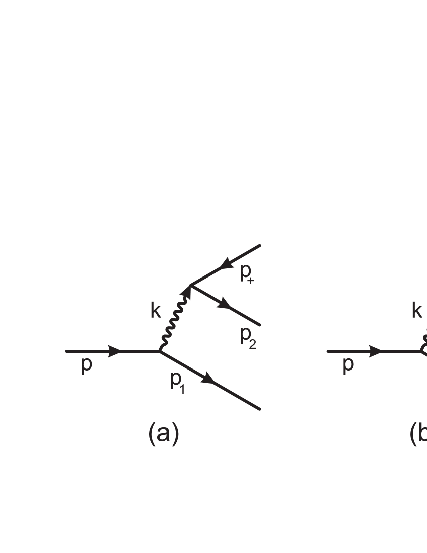
Figure 1: Direct (a) and exchange (b) Feynman diagrams for the electron–positron pair production by an electron in a magnetic field.

Let us choose a coordinate system in which the magnetic field $\vec{H}$ is directed along the $z$ axis. The eigenvalues of the electron energy in the magnetic field are then

$$E_{l}=\sqrt{p_{z}^{2}+m^{2}+m^{2}2lh}.$$ (2)

Here, $l$ is the Landau level number and $p_{z}$ is the $z$ component of the electron momentum.

The magnetic field does not change in going to the frame of reference that moves along the $z$ axis. Therefore, without any loss of generality, the longitudinal component of the initial electron momentum may be set equal to zero: $p_{z}=0$. Consequently,

$$E=\tilde{m}=m\sqrt{1+2lh}$$ (3)

for the initial electron.

The kinematics of the process is defined by the following conservation laws:

$$\left\{\begin{array}[]{l}E_{1}+E_{2}+E_{+}=E,\\ p_{1z}+p_{2z}+p_{+z}=p_{z}=0,\end{array}\right.$$ (4)

where $E$ and $p_{z}$ are the energy and longitudinal momentum of the initial electron; $E_{1}$, $E_{2}$ and $E_{+}$ are the energies of the final electrons and positron; $p_{1z}$, $p_{2z}$ and $p_{+z}$ are their longitudinal momenta.

First of all, note that the process is impossible if the initial electron energy is insufficient for pair production. It is easy to verify that the threshold condition is

$$\left\{\begin{array}[]{l}p_{1z}=p_{2z}=p_{+z}=0,\\ \tilde{m}=\tilde{m}_{1}+\tilde{m}_{2}+\tilde{m}_{+}.\end{array}\right.$$ (5)

Generally, this condition cannot be met, because the effective masses are discrete quantities. Thus, the threshold values of the longitudinal momenta of the final particles are nonzero. Expanding Eq. (4) into a series of momenta, we will obtain the relation

$$\frac{p_{1z}^{2}}{b_{1}^{2}}+\frac{p_{2z}^{2}}{b_{2}^{2}}+\frac{p_{+z}^{2}}{b_{+}^{2}}=1,$$ (6)

where

$$b_{f}^{2}=2\tilde{m}_{f}\Delta,$$

$$\Delta=\tilde{m}-\tilde{m}_{1}-\tilde{m}_{2}-\tilde{m}_{+},$$

and the subscript $f$ numbers the final particles ($f=1,\,2,\,+$).

It is easy to verify that at the process threshold when

$$l_{f}=0,$$ (7)

the following conditions are met:

$$\begin{array}[]{l}\tilde{m}_{f}=m,\\ \Delta\leq mh,\\ p_{fz}\lesssim m\sqrt{h}.\end{array}$$ (8)

In the coordinate system where the momenta $p_{1z}$, $p_{2z}$ and $p_{+z}$ are along the axes, the energy conservation law (6) specifies an ellipsoid. The possible values of the momenta correspond to the points of the ellipse formed by the intersection of ellipsoid (6) with the plane specified by the momentum conservation law (Fig. 2):

$$p_{1z}+p_{2z}+p_{+z}=0.$$ (9)

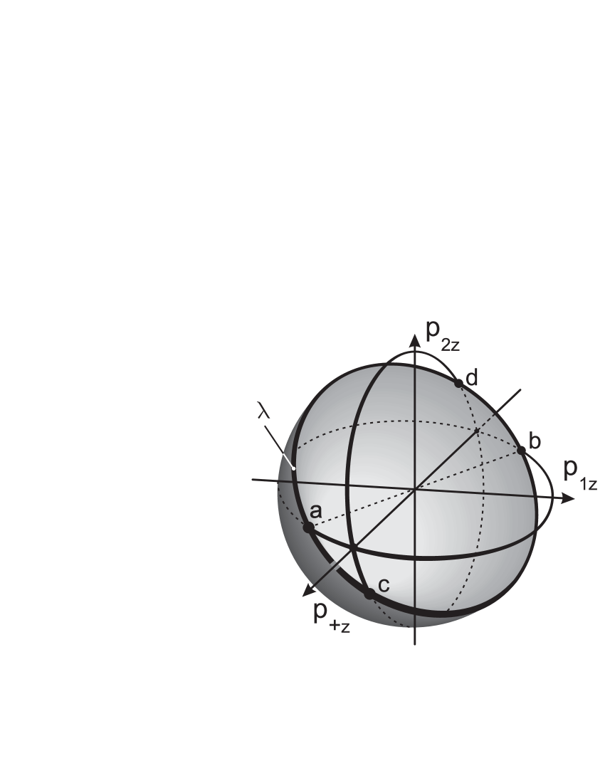
Figure 2: Threshold particle momenta – the points of ellipse $\lambda$. Points a, b and c, d are the points of intersection of ellipse $\lambda$ with the $(p_{+z},p_{1z})$ and $(p_{2z},p_{+z})$ planes, respectively.

III THE PROBABILITY OF THE PROCESS

According to general rules of quantum electrodynamics, the probability amplitude for the process is

$$\begin{array}[]{l}\displaystyle S_{fi}=i\alpha\int\!\!\int d^{4}xd^{4}x^{\prime}\left[(\bar{\Psi}_{2}\gamma^{\mu}\Psi)D_{\mu\nu}(\bar{\Psi}_{1}^{\prime}\gamma^{\nu}\Psi_{+}^{\prime})-\right.\\ \left.-(\bar{\Psi}_{1}\gamma^{\mu}\Psi)D_{\mu\nu}(\bar{\Psi}_{2}^{\prime}\gamma^{\nu}\Psi_{+}^{\prime})\right].\end{array}$$ (10)

Here, the prime on the wave function means that it depends on the components of the primed 4-radius vector $x^{\prime}$. Let us substitute the wave functions Fomin2000 and the photon propagator Landau4 into the amplitude:

$$D_{\mu\nu}=\frac{g_{\mu\nu}}{(2\pi)^{4}}\int{d^{4}ke^{-ik(x-x^{\prime})}\frac{4\pi}{k^{j}k_{j}}}.$$ (11)

Since the dependencies of the wave functions on time and $y$, $z$, $y^{\prime}$, and $z^{\prime}$ coordinates are the same in form as those for plane waves, integration over these quantities gives $\delta$-functions that express the energy and momentum conservation laws. The integrals over the $x$ and $x^{\prime}$ coordinates can be expressed in terms of special functions studied in Klepikov ; FIAN . Substituting their explicit form at $l_{f}=0$ yields the following expression for the probability amplitude of the process:

$$S_{fi}=S_{1}-S_{2}.$$ (12)

Here,

$$\begin{array}[]{l}\displaystyle S_{1}=\frac{i\alpha\,2\pi^{3}}{S^{2}\sqrt{\tilde{m}EE_{1}E_{2}E_{+}}}\frac{B_{1}^{\pm}\sqrt{\tilde{m}-\mu m}}{m\sqrt{l!h}}e^{-a^{2}}X_{1}\times\\ \times\delta(E\!-\!E_{1}\!-\!E_{2}\!-\!E_{+})\delta(p_{y}\!-\!p_{1y}\!-\!p_{2y}\!-\!p_{+y})\times\\ \delta(p_{z}-p_{1z}-p_{2z}-p_{+z}),\end{array}$$

$S_{2}$ is the exchange term,

$$X_{1}=\int{\frac{(a+i\xi)^{l}}{\rho^{2}-\xi^{2}}e^{-\xi^{2}-2ib\xi}d\xi},$$ (13)

$$\begin{array}[]{l}a=(p_{y}-p_{1y})/m\sqrt{2h},\\ b=(p_{y}-p_{2y})/m\sqrt{2h},\\ \xi=k_{x}/m\sqrt{2h},\\ \rho^{2}=\Omega^{2}-a^{2},\quad\Omega^{2}=h/2,\end{array}$$ (14)

$$B_{1}^{+}=4m\sqrt{m\tilde{m}},\quad B_{1}^{-}=4p_{1z}\sqrt{m\tilde{m}}.$$ (15)

We will obtain the probability of the process by multiplying the square of the absolute value of the amplitude by the number of final states:

$$dW=|S_{fi}|^{2}\frac{Sd^{2}p_{1}}{(2\pi)^{2}}\frac{Sd^{2}p_{2}}{(2\pi)^{2}}\frac{Sd^{2}p_{+}}{(2\pi)^{2}},$$ (16)

where $d^{2}p_{f}=dp_{fy}\,dp_{fz}$.

Squaring the absolute value of (12) yields the differential probability of the process per unit time

$$\begin{array}[]{l}dW=M\left|e^{-a^{2}}X_{1}B_{1}^{\pm}-e^{-b^{2}}X_{2}B_{2}^{\pm}\right|^{2}\times\\ \delta(E\!-\!E_{1}\!-\!E_{2}\!-\!E_{+})\delta(p_{y}\!-\!p_{1y}\!-\!p_{2y}\!-\!p_{+y})\times\\ \delta(p_{z}-p_{1z}-p_{2z}-p_{+z})d^{2}p_{1}d^{2}p_{2}d^{2}p_{+},\end{array}$$ (17)

where

$$M=\frac{\alpha^{2}(\tilde{m}-\mu m)}{2^{7}\pi^{3}m^{2}\tilde{m}EE_{1}E_{2}E_{+}hl!}.$$ (18)

The integration over $d^{2}p_{+}$ can be easily performed using the $\delta$-functions $\delta(p_{y}-p_{1y}-p_{2y}-p_{+y})\delta(p_{z}-p_{1z}-p_{2z}-p_{+z})$. The probability then takes the form

$$\begin{array}[]{l}dW=2m^{2}hM\left[\left((B_{1}^{\pm})^{2}+(B_{2}^{\pm})^{2}\right)Y-2B_{1}^{\pm}B_{2}^{\pm}Y^{\prime}\right]\times\\ \delta(E-E_{1}-E_{2}-E_{+})dp_{1z}dp_{2z},\end{array}$$ (19)

where we introduced the designations

$$\begin{array}[]{l}Y=\int\int da\,db\left|e^{-a^{2}}X_{1}\right|^{2},\\ Y^{\prime}=\int\int da\,db\,e^{-a^{2}-b^{2}}Re(X_{1}X_{2}^{*}).\end{array}$$ (20)

The quantity $Y^{\prime}$ defines the interference term in the probability of the process.

In Eq. (19), we will transform the $\delta$ function of the particle energies to the $\delta$ function of the momentum components

$$\delta(E-E_{1}-E_{2}-E_{+})=\frac{m\sum\limits_{j=\pm}{\delta(p_{1z}-g_{j})}}{\sqrt{4m\Delta-3p_{2z}^{2}}},$$ (21)

where

$$g_{\pm}=\frac{1}{2}\left(-p_{2z}\pm\sqrt{4m\Delta-3p_{2z}^{2}}\right).$$

In view of the chosen conditions (1), (7), and (8), the dependence of the probability on the $z$ momentum components can be neglected everywhere, except the factors $B_{1}^{-}$ and $B_{2}^{-}$, and the $\delta$ function (21). Therefore, the probability (19) can be easily integrated in finite form. As a result, we will obtain the expressions

$$W^{+}=\frac{\alpha^{2}2m}{3\pi^{2}\sqrt{3}l!}(Y-Y^{\prime}),$$ (22)

$$W^{-}=\frac{\alpha^{2}4\Delta}{9\pi^{2}\sqrt{3}l!}(2Y+Y^{\prime}).$$ (23)

Let us calculate $Y$ and $Y^{\prime}$. First of all, note that we can generally assume from physical considerations that $a\sim\xi$. Therefore, the middle term with $\xi^{l/2}$ makes a major contribution in the expansion of the binomial in Eq. (13). In addition, a numerical analysis of this expression shows that the principal-value integral can be neglected compared to the pole residue. Using these assumptions, we can easily calculate the integral $X_{1}$ and then obtain the following result for $Y$ and $Y^{\prime}$:

$$\begin{array}[]{l}\displaystyle Y=4\sqrt{2}\pi^{2}\Omega^{2l}e^{-2\Omega^{2}}\frac{l!}{l\Gamma(l/2+1)^{2}},\\ Y^{\prime}\ll Y,\end{array}$$ (24)

where $\Gamma$ is the gamma function.

Substituting $Y$ into Eqs. (22) and (23) and neglecting the interference term, we will obtain the final expressions for the total probability of the process (per unit time, $s^{-1}$)

$$W^{+}=\alpha^{2}\left(\frac{mc^{2}}{\hbar}\right)\frac{8\sqrt{2}}{3\sqrt{3}}\,\,\frac{\Omega^{2l}e^{-2\Omega^{2}}}{l\Gamma(l/2+1)^{2}},$$ (25)

$$W^{-}=\alpha^{2}\left(\frac{mc^{2}}{\hbar}\right)\frac{\Delta}{m}\frac{32\sqrt{2}}{9\sqrt{3}}\,\,\frac{\Omega^{2l}e^{-2\Omega^{2}}}{l\Gamma(l/2+1)^{2}}.$$ (26)

IV ANALYSIS OF THE PROBABILITY

Let us analyze the result obtained. First of all, note that the total probability contains no singularities, when the longitudinal particle momenta are zero, characteristic of the photoproduction process $\gamma\rightarrow ee^{+}$ Shabad ; HardingRep ; Novak .

From Eqs. (25) and (26), it is easy to derive the ratio of the probabilities

$$\frac{W^{-}}{W^{+}}=\frac{4}{3}\frac{\Delta}{m},$$ (27)

where $\Delta=E-3m$. As was pointed out previously, $\Delta\lesssim mh$ near the process threshold and, hence, $W^{-}\ll W^{+}$. In the special case where the magnetic field is $h=4/l$, the equality $\Delta=0$ holds and, hence, $W^{-}=0$ (within the accuracy of the approximation).

In Fig. 3, the total probability is plotted against the Landau level number for the initial electron. The magnetic field is taken to be $h=0.1$, with the threshold value of the Landau level for the initial electron being $l=40$. As we see, the probability of the process is $10^{13}$ $c^{-1}$:

$$W^{+}\sim 10^{13}\,\,c^{-1}.$$ (28)

Both probabilities decrease with increasing number $l$ and $W^{-}$ approaches zero near the threshold.

In conclusion, let us compare the probability of the process considered with the probabilities of other processes. The table gives the probabilities of the following processes: emission, photoproduction, double synchrotron emission (this process in the field of a laser wave was considered in Voroshilo ; Lotstedt ), photoproduction with photon emission, and pair production by an electron. The magnetic field is $h=0.1$ ($\approx 4.4\cdot 10^{12}$ G).

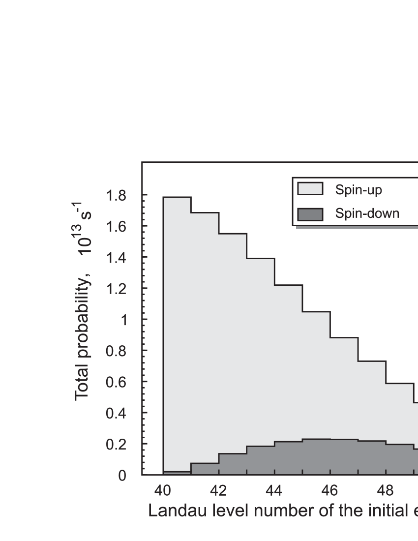
Figure 3: Total probability of pair production at the ground levels versus Landau level number for the initial electron, $h=0.1$.

Table 1: Comparison of the probabilities of various processes, $h=0.1$.

	a	b	c	d	e
Process	Emission	Photoproduction	Double emission	Photoproduction with emission	Pair production by electron
Diagram
Initial conditions	${l=40}$, ${l^{\prime}=0}$	${\omega=2m}$, ${l_{-}=l_{+}=0}$	Lowest levels	Lowest levels	${l=40}$, ${E=2m}$, ${l_{f}=0}$
Probability, ${s^{-1}}$	$\begin{array}[]{l}\!\!W_{e\rightarrow\gamma e}^{total}\sim 10^{17}\\ \!\!W_{e\rightarrow\gamma e}^{\omega>2m}\sim 10^{14}\\ \!\!W_{e\rightarrow\gamma e}^{1\rightarrow 0}\sim 10^{16}\end{array}$	${W_{\gamma\rightarrow ee^{+}}\sim 10^{9}}$	${W_{e\rightarrow e\gamma\gamma}^{res}\sim W_{e\rightarrow\gamma e}^{1\rightarrow 0}}$	$\begin{array}[]{l}\!\!W_{\gamma\rightarrow\gamma ee^{+}}^{nonres}\sim 10^{6}\\ \!\!W_{\gamma\rightarrow\gamma ee^{+}}^{res}\sim W_{\gamma\rightarrow ee^{+}}\end{array}$	$W\sim 10^{13}$
References	Klepikov ; Novak ; Kholodov2001	Klepikov ; HardingRep ; Baier ; Novak2008 ; Novak	Fomin2003	Fomin2007	–

For the photoproduction probability, we use an expression derived in the ultraquantum approximation Novak2008 ; Novak . Let us take the initial photon frequency to be $\omega=2m$, the electron and positron level numbers to be $l_{f}=0$, and the magnetic field to be $h=0.1$. The photoproduction probability has a resonant pattern and depends significantly on the $z$ component of the particle momenta. We will choose them to be of the order of $m\sqrt{h}$ based on our estimate of (8). Then,

$$W_{\gamma\rightarrow ee^{+}}\approx 3.7\cdot 10^{9}c^{-1}.$$

To estimate the emission probability, it is necessary to use the ultrarelativistic approximation Klepikov ; Novak . Choosing the initial electron energy to be $3m$, we will obtain an estimate of the total synchrotron emission probability:

$$W_{e\rightarrow\gamma e}^{total}\sim 2.8\cdot 10^{17}c^{-1}.$$

However, this includes the processes of photon emission with an energy insufficient for pair production. The probability of emitting a photon with an energy from $2m$ to $\omega_{max}\approx 3m$ is

$$W_{e\rightarrow\gamma e}^{\omega>2m}\sim 6.8\cdot 10^{14}c^{-1}.$$

- (1) S. Shapiro and S. Teukolsky, Black Holes, White Dwarfs, and Neutron Stars (Wiley, New York, 1983; Mir, Moscow, 1985).
- (2) A. K. Harding, A. G. Muslimov, B. Zhang, The Astrophysical Journal, 576 366 (2002).
- (3) N. Harrison and S. Crooker, Mag Lab Reports 14 (1), 11 (2007).
- (4) A. D. Sakharov, Usp. Fiz. Nauk 161 (5), 29 (1991) [Sov. Phys.—Usp. 34 (5), 375 (1991)].
- (5) D. L. Burke, R. C. Field, G. Horton-Smith, J. E. Spencer, D. Walz, S. C. Berridge, W. M. Bugg, K. Shmakov, A. W. Weidemann, C. Bula, K. T. McDonald, E. J. Prebys, C. Bamber, S. J. Boege, T. Koffas, T. Kotseroglou, A. C. Melissinos, D. D. Meyerhofer, D. A. Reis, and W. agg, Phys. Rev. Lett. 79, 1626 (1997).
- (6) I. Koenig, E. Berdermann, F. Bosch, P. Kienle, W. Koenig, C. Kozhuharov, A. Schroter, and H. Tsertos, Z. Phys. A 346 153 (1993).
- (7) N. P. Klepikov, Zh. Eksp. Teor. Fiz. 26, 19 (1954).
- (8) A. I. Nikishov, Tr. Fiz. Inst. im. P. N. Lebedeva, Akad. Nauk SSSR 111, 152 (1979).
- (9) C. Graziani, A. K. Harding and R. Sina, Phys. Rev. D 51, 7097 (1995).
- (10) P. I. Fomin and R. I. Kholodov, Zh. Eksp. Teor. Fiz. 117(2), 319 (2000) [JETP 90 (2), 281 (2000)].
- (11) L. D. Landau and E. M. Lifshitz, Course of Theoretical Physics, Vol. 4: V. B. Berestetskii, E. M. Lifshitz, and L. P. Pitaevskii, Quantum Electrodynamics (Fizmatlit, Moscow, 2001; Butterworth-Heinemann, Oxford, 2002).
- (12) A. E. Shabad, Tr. Fiz. Inst. im. P. N. Lebedeva, Akad. Nauk SSSR 192, 5 (1988).
- (13) A. K. Harding, Phys. Rep. 206(6), 327 (1991).
- (14) O. P. Novak, R. I. Kholodov, Phys. Rev. D 80(2) 025025 (2009).
- (15) O. I. Voroshilo and S. P. Roshchupkin, Probl. At. Sc. Thech. 3(1) 221 (2007).
- (16) E. Lötstedt and U. D. Jentschura, Phys. Rev. Lett. 103(11) 110404 (2009).
- (17) O. P. Novak, R. I. Kholodov, Ukr. J. Phys. 53(2) 185 (2008).
- (18) R. I. Kholodov, P. V. Baturin, Ukr. J. Phys. 46(5-6) 621 (2001).
- (19) V. N. Baier and V. M. Katkov, Phys. Rev. D 75(7) 073009 (2007).
- (20) P. I. Fomin and R. I. Kholodov, Zh. Eksp. Teor. Fiz. 123 (2), 356 (2003) [JETP 96 (2), 315 (2003)].
- (21) P. I. Fomin, R. I. Kholodov, Probl. At. Sci. Thechnol. 3 179 (2007).