Magnet field sensing beyond the standard quantum limit under the effect of decoherence

Abstract

Entangled states can potentially be used to outperform the standard quantum limit which every classical sensor is bounded by. However, entangled states are very susceptible to decoherence, and so it is not clear whether one can really create a superior sensor to classical technology via a quantum strategy which is subject to the effect of realistic noise. This paper presents an investigation of how a quantum sensor composed of many spins is affected by independent dephasing. We adopt general noise models including non-Markovian effects, and in these noise models the performance of the sensor depends crucially on the exposure time of the sensor to the field. We have found that, by choosing an appropriate exposure time within non-Markovian time region, an entangled sensor does actually beat the standard quantum limit. Since independent dephasing is one of the most typical sources of noise in many systems, our results suggest a practical and scalable approach to beating the standard quantum limit.

Entanglement has proven itself to be one of the most intriguing aspects of quantum mechanics, and its study has lead to profound advances in our understanding of physics. Aside from these conceptual advances, the exploitation of entanglement has lead to a number of technical advances both in computation and communication Nielsen and Chuang (2000), and more recently in metrology Giovannetti et al. (2004). In quantum metrology, entanglement has been used to demonstrate enhanced accuracy both in detecting the phase induced by unknown optical elements and for accurately measuring an unknown magnetic field. It is this latter case which is the focus of the present paper, and so we will adopt the terminology of field sensing.

In order to estimate an unknown field, one usually prepares a probe system composed of $L$ distinct local subsystems, exposes this to the field for a certain time, and measures the probe. Comparing the input with the output of the probe gives us an estimate of the field. Importantly, there is an uncertainty in the estimation, and this uncertainty is related to how the probe system is prepared. When the probe system is prepared in a separable state, the uncertainty decreases as $1/\sqrt{L}$ Pezzé and Smerzi (2009); Itano et al (1993) by the central limit theorem, a scaling known as the standard quantum limit. On the other hand, by preparing a highly entangled state, it is in principal possible to achieve an uncertainty that scales as $1/L$, known the Heisenberg limit Giovannetti et al. (2004, 2006).

Most of the literature on quantum sensing focuses on using photons to probe an unknown optical element. Using a NOON state Nagata et al (2007); Afek et al. (2010); Kok et al. (2002), it is possible to measure the unknown phase shift with higher resolution than the standard quantum limit. An $L$-photon NOON state can achieve a phase $L$ times as large as than in the case of a single photon over the same channel. Recent publications Leibfried et al (2005); Jones et al (2009); Leibfried et al. (2004); Schaffry et al. (2010) have considered an analogous technique for field sensing with spins. In this paper, we consider an experiment involving a probe consisting of spin-$\frac{1}{2}$ systems. The spin qubits can couple to the magnetic field and therefore one can estimate the value of the magnetic field by the probe. In order to obtain higher resolution than the standard quantum limit, one can use a GHZ state, as has been demonstrated in recent experiments Leibfried et al (2005); Jones et al (2009); Simmons et al. (2009); Leibfried et al. (2004).

In solid state systems, one of the main barriers to realising such sensors is decoherence, which degrades the quantum coherence of the entangled states. GHZ states, in particular, are very susceptible to decoherence, and decohere more rapidly as the size of the state increases Dur and Briegel (2004); Shaji and Caves (2007). Therefore, it is not clear whether a quantum strategy can really outperform an optimal classical strategy under the effects of a realistic noise source. The effect of unknown but static field variations over the L spins has been studied by Jones et al Jones et al (2009). The uncertainty of the estimation depends on the exposure time of entangled states to the field, where they are affected by noise, and they have found that, for an optimal exposure time in their model, the scaling of the estimated value is $L^{-\frac{3}{4}}$ which beats the standard quantum limit. However, the underlying assumption that the fields are static could be unrealistic for many systems, as actual noise in the laboratory may fluctuate with time. Huelga et al have included such temporal fluctuations of the field in their noise model Huelga et al. (1997) and have shown that GHZ states cannot beat the standard quantum limit under the effect of independent dephasing by adopting a Lindblad type master equation Huelga et al. (1997). Even for the optimal exposure time, it was shown that the measurement uncertainty of a quantum strategy has the same scaling behavior as the standard quantum limit in their noise model. Since independent dephasing is the dominant error sources in many systems, these results seem to show that, practically, it would be impossible to beat the standard quantum limit with a quantum strategy.

However, the model adopted by Huelga et al is a Markovian master equation Gardiner and Zoller (2004) which is valid in limited circumstances. The Markovian assumption will be violated when the correlation time of the noise is longer than the characteristic time of the system. For example, although a Markovian master equation predicts an exponential decay behavior, it is known that unstable systems show a quadratic decay in the time region shorter than a correlation time of the noise Nakazato et al. (1996); Schulman (1997). In this paper, we adopt independent dephasing models which include non-Markovian effects and we investigate how the uncertainty of the estimation is affected by such noise. We have found that, if the exposure time of the entangled state is within the non-Markovian region, a quantum strategy can indeed provide a scaling advantage over the optimal classical strategy.

Let us summarize a quantum strategy to obtain the Heisenberg limit in an ideal situation without decoherence. A state prepared in $|+\rangle=\frac{1}{\sqrt{2}}(|0\rangle+|1\rangle)$ will have a phase factor in its non-diagonal term through being exposed in a magnetic field and so we have $\frac{1}{\sqrt{2}}(|0\rangle+e^{-it\delta}|1\rangle)$ where $\delta$ denotes the detuning between the magnetic field and the atomic transition. On the other hand, when one prepares a GHZ state $|\psi\rangle_{\text{GHZ}}=\frac{1}{\sqrt{2}}(|00\cdots 0\rangle+|11\cdots 1\rangle)$ and exposes this state to the field for a time $t$, the phase factor is amplified linearly as the size of the state increases as

$$|\psi(t)\rangle=\frac{1}{\sqrt{2}}(|00\cdots 0\rangle+e^{-iLt\delta}|11\cdots 1\rangle).$$ (1)

Therefore, the probability of finding the initial GHZ state after a time $t$ is given by $P=\frac{1}{2}+\frac{1}{2}\cos(Lt\delta)$. In practice, one may use control-not operations to map the accumulated phase to a single spin for a convenient measurement Jones et al (2009). The variance of the estimated value is then given by

$$\Delta^{2}\delta=\frac{P(1-P)/N}{|dP/d\delta|^{2}}$$ (2)

where $N$ is the number of experiments performed in this setting Huelga et al. (1997). For a given fixed time $T$, one can perform this experiment $T/t$ times where $t$ is the exposure time, and so we have $N=T/t$. Hence we obtain $|\Delta^{2}\delta|=\frac{1}{TL^{2}t}$ and so the uncertainty in $\delta$ scales as $L^{-1}$, the Heisenberg limit.

First let us consider the decoherence of a single qubit. Later, we will generalize to GHZ states. Our noise model represents random classical fields to induce dephasing. We consider an interaction Hamiltonian to denote a coupling with an environment such as

$$H_{I}=\lambda f(t)\hat{\sigma}_{z}$$ (3)

where $f(t)$ is classical normalized Gaussian noise, $\hat{\sigma}_{z}$ is a Pauli operator of the system, and $\lambda$ denotes a coupling constant. Also, we assume symmetric noise to satisfy $\overline{f(t)}=0$ where this over-line denotes the average over the ensemble of the noise. When we solve the Schrödinger equation in an interaction picture, we obtain the following standard form

$$\rho_{I}(t)-\rho_{0}=\sum_{n=1}^{\infty}(-i\lambda)^{n}\int_{0}^{t}dt_{1}\int_{0}^{t_{1}}dt_{2}\cdots\int_{0}^{t_{n-1}}dt_{n}$$

$$[H_{I}(t_{1}),[H_{I}(t_{2}),\cdots,[H_{I}(t_{n}),\rho_{0}]\cdots]]$$ (4)

where $\rho_{0}=|\psi\rangle\langle\psi|$ is an initial state and $\rho_{I}(t)$ is a state in the interaction picture. Throughout this paper, we restrict ourselves to the case where the system Hamiltonian commutes with the operator of noise, as this constitutes purely dephasing noise. By taking the average over the ensemble of the noise, we obtain

$$\rho_{I}(t)-\rho_{0}=\sum_{n=1}^{\infty}\frac{1}{n!}(-i\lambda)^{n}\int_{0}^{t}dt_{1}\int_{0}^{t}dt_{2}\cdots\int_{0}^{t}dt_{n}$$

$$\overline{f(t_{1})f(t_{2})\cdots f(t_{n})}[\hat{\sigma}_{z},[\hat{\sigma}_{z},\cdots,[\hat{\sigma}_{z},\rho_{0}]\cdots]]_{n}$$ (5)

where $[\hat{\sigma}_{z},[\hat{\sigma}_{z},\cdots,[\hat{\sigma}_{z},\rho_{0}]\cdots]]_{n}$ denotes the $n$-folded commutator of $\rho_{0}$ with $\hat{\sigma}_{z}$. Since all higher order cumulants than the second order are zero for Gaussian noise, $\overline{f(t_{1})f(t_{2})\cdots f(t_{n})}$ can be represented by a product of correlation functions Meeron (1957). Therefore, the decoherence caused by Gaussian noise is characterized by a correlation function of the noise. For Markovian white noise, a correlation function becomes a delta function while a correlation function becomes a constant for non-Markovian noise with an infinite correlation time such as $1/f$ noise. To include both noise models as special cases, we assume the correlation function

$$\overline{f(t_{1})f(t_{2})}=\frac{2}{\sqrt{\pi}}e^{-\frac{|t_{1}-t_{2}|^{2}}{\tau_{c}^{2}}},$$ (6)

where $\tau_{c}$ denotes the correlation time of the noise. In the limit $\tau_{c}\rightarrow 0$, this correlation function becomes a delta function, while in the limit of $\tau_{c}\rightarrow\infty$ it becomes constant.

Since $\overline{f(t_{1})f(t_{2})\cdots f(t_{n})}$ can be represented by a product of correlation functions, we obtain

$$\rho_{I}(t) = \sum_{n=0}^{\infty}\frac{(-\frac{1}{4}t\gamma(t))^{n}}{n!}[\hat{\sigma}_{z},[\hat{\sigma}_{z},\cdots,[\hat{\sigma}_{z},\rho_{0}]\cdots]]_{2n}$$ (7)

$$= \sum_{s,s^{\prime}=\pm 1}e^{-\frac{1}{4}|s-s^{\prime}|^{2}\gamma(t)t}|s\rangle\langle s|\rho_{0}|s^{\prime}\rangle\langle s^{\prime}|$$

where $|s\rangle$ is an eigenvector of $\hat{\sigma}_{z}$. Also, $\gamma(t)$ denotes the single qubit decoherence rate defined as

$$\gamma(t)=\frac{4\lambda^{2}\tau_{c}^{2}(-1+e^{-\frac{t^{2}}{\tau_{c}^{2}}})}{\sqrt{\pi}t}+4\lambda^{2}\tau_{c}\text{erf}(\frac{t}{\tau_{c}})$$ (8)

where $\text{erf}(x)$ is the error function. Note that, for $t\gg\tau_{c}$, the decoherence rate becomes constant as $\gamma(t)\simeq 4\lambda^{2}\tau_{c}$. So, in this regime, we can derive a Markovian master equation from (7), which has the same form as adopted by Huelga et al Huelga et al. (1997).

$$\frac{d\rho_{I}(t)}{dt}\simeq-\lambda^{2}\tau_{c}[\hat{\sigma}_{z}[\hat{\sigma}_{z},\rho_{I}(t)]]\ \ (t\gg\tau_{c})$$ (9)

Note that, although our model can be approximated by Markovian noise in the long time limit ($t\gg\tau_{c}$), we are interested in the time periods $t\sim\tau_{c}$ and $t\ll\tau_{c}$ where non-Markovian effects become relevant.

For an initial state $|+\rangle=\frac{1}{\sqrt{2}}(|0\rangle+|1\rangle)$, the non-diagonal terms of the density matrix show a decay behavior of $\langle 0|\rho_{I}(t)|1\rangle=\frac{1}{2}\text{exp}[-\gamma(t)t]$.

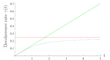
Figure 1: We have plotted the behavior of a single qubit decoherence rate for $1/f$ noise $\frac{4}{\sqrt{\pi}}\lambda^{2}t$ (the green line), Markovian noise $4\lambda^{2}\tau_{c}$ (the red line), and our classical noise model (blue dotted line) $\gamma(t)$ defined in (8) where $\lambda$ and $\tau_{c}$ denote a coupling constant with the environment and a correlation time of the noise, respectively. For an $L$-qubit GHZ state, the decoherence rate becomes $L$ times greater than the value plotted here. Note that our noise model shows a transition from a non-Markovian quadratic decay to an exponential Markovian decay. Here, we fixed parameters as $\lambda=0.25$ and $\tau_{c}=1$.

For $t\gg\tau_{c}$, the state shows an exponential decay $\langle 0|\rho_{I}(t)|1\rangle\simeq\frac{1}{2}e^{-4\lambda^{2}\tau_{c}t}$. On the other hand, we have $\langle 0|\rho_{I}(t)|1\rangle\simeq\frac{1}{2}e^{-\frac{4}{\sqrt{\pi}}\lambda^{2}t^{2}}$ (quadratic decay behavior) for $t\ll\tau_{c}$ , which is the typical decay behavior of $1/f$ noise Yoshihara et al. (2006); Kakuyanagi et al. (2007); Matsuzaki et al. (2010). The behavior of the decoherence rate is illustrated in Fig. 1.

We next consider decoherence of a GHZ state induced by random classical fields. Extending the Hamiltonian in (3), the interaction Hamiltonian denoting random classical fields for a many-qubit system is as follows:

$$H_{I}=\lambda\sum_{l=1}^{L}f_{l}(t)\hat{\sigma}_{z}(l)$$ (10)

where $f_{l}(t)$ denotes the noise acting at site $l$ and has the same characteristics as $f(t)$ mentioned above. Also, since we consider independent noise, we have $\overline{f_{l}(t)f_{l^{\prime}}(t^{\prime})}\propto\delta_{l,l^{\prime}}$. When we let a GHZ state be exposed to a magnetic field under the effect of the random magnetic fields, the state will remain in the subspace spanned by $\bigotimes^{L}_{l=1}|0\rangle_{l}$ and $\bigotimes^{L}_{l=1}|1\rangle_{l}$ because we are only considering phase noise. Thus, we can use the same analysis as for a single qubit. In the the Schrödinger picture, we will obtain

$$\rho(t)=\frac{1}{2}\big{(}\bigotimes^{L}_{l=1}|0\rangle_{l}\langle 0|\big{)}+\frac{1}{2}e^{iLt\delta-L\gamma(t)t}\big{(}\bigotimes^{L}_{l=1}|0\rangle_{l}\langle 1|\big{)}$$ (11)

$$+ \frac{1}{2}e^{-iLt\delta-L\gamma(t)t}\big{(}\bigotimes^{L}_{l=1}|1\rangle_{l}\langle 0|\big{)}+\frac{1}{2}\big{(}\bigotimes^{L}_{l=1}|1\rangle_{l}\langle 1|\big{)}$$

where $\delta$ is the phase induced by the magnetic field to be measured. It is worth mentioning that the decoherence rate for a $L$-qubit GHZ state becomes $L$ times the decoherence rate $\gamma(t)$ of a single qubit. Therefore, the variance of the estimated value becomes

$$\Delta^{2}\delta = \frac{e^{2\gamma(t)Lt}-1}{TL^{2}t\sin^{2}(Lt\delta)}+\frac{1}{TL^{2}t}$$ (12)

where we use (2), and therefore we obtain the following inequality by using $x\geq\sin x\geq\frac{2}{\pi}x$ for $0\leq x\leq\frac{\pi}{2}$:

$$\frac{e^{2\gamma(t)Lt}-1}{TL^{4}t^{3}\delta^{2}}\leq(\Delta^{2}\delta)-\frac{1}{TL^{2}t}\leq\frac{\pi^{2}(e^{2\gamma(t)Lt}-1)}{4TL^{4}t^{3}\delta^{2}}$$ (13)

These inequalities depend on both the system size $L$ and the choice of exposure time $t$. We wish to see if there is any choice of $t$ for which we beat the standard quantum limit. We find that this limit can indeed be beaten provided that we chose shorter $t$ values for larger systems. For example, suppose that we chose $t$ according to the rule $t=sL^{-z}$, where $s$ is a constant with the dimension of time, and $z$ is a non-negative real number whose optimal value we will determine. Then, from (8), we have

$$|\gamma(t)-\frac{4s\lambda^{2}}{\sqrt{\pi}L^{z}}|\leq\frac{12s^{2}\lambda^{2}/\tau_{c}}{\sqrt{\pi}L^{z}(L^{2z}-s^{2}/\tau_{c}^{2})}$$ (14)

for large $L$ and hence the decoherence rate scales as $\gamma(t)=\Theta(L^{-z})$. Throughout this paper, for a function $f(L)$, we say $f(L)=\Theta(L^{n})$ if there exists positive constants $J$ and $K$ such that $JL^{n}\leq f(L)\leq KL^{n}$ is satisfied for all $L$.

In (13), the term in the exponential $\gamma(t)tL$ goes to infinity as $L\rightarrow\infty$ for $z<1/2$, and so the uncertainty $|\Delta^{2}\delta|$ diverges, which means that a large GHZ state becomes useless to estimate $\delta$. Therefore, we consider the case of $z\geq 1/2$. By performing a Taylor expansion of $e^{2\gamma(t)Lt}$, we obtain

$$\frac{e^{2\gamma(t)Lt}-1}{L^{4}t^{3}}=\sum_{n=1}^{\infty}\frac{(2\gamma(t)Lt)^{n}}{L^{4}t^{3}\cdot n!}=\Theta(L^{z-3})\ \ \ \ \$$ (15)

for $z\geq 1/2$ where we use (14).

So, from (13) and (15), we obtain

$$\Delta^{2}\delta=\Theta(L^{-2+z})$$ (16)

for $z\geq\frac{1}{2}$. Therefore, when $z=\frac{1}{2}$, we achieve a scaling of the uncertainty $|\Delta\delta|=\Theta(L^{-\frac{3}{4}})$ and this actually beats the standard quantum limit. Note that this is the same scaling as the magnetic sensor under the effect of unknown static fields studied in Jones et al (2009), and so our result for the fluctuating noise with time becomes a natural generalization of their work.

The decoherence model described above is a classical one. Next, we make use of a quantized model where the environment is modeled as a continuum of field modes. The Hamiltonian of the system and the environment are defined as

$$H=\frac{\delta}{2}\sum_{l=1}^{L}\hat{\sigma}_{z}(l)+\sum_{l,{{k}}}\omega_{{{k}}}\hat{b}^{\dagger}_{l,{{k}}}\hat{b}_{l,{{k}}}+\sum_{l,{{k}}}g_{{{k}}}\hat{\sigma}_{z}(l)\hat{b}^{\dagger}_{l,{{k}}}\hat{b}_{l,{{k}}}$$ (17)

where $\hat{b}_{l,{{k}}}$ and $\hat{b}^{\dagger}_{l,{{k}}}$ denote annihilation and creation operators for the bosonic field at a site $l$. Also, since we consider independent noise, we assume that $\hat{b}_{l,{{k}}}$ commutes with $\hat{b}^{\dagger}_{l^{\prime},{{k}}}$ for $l\neq l^{\prime}$. This model has been solved analytically by Palma et al Palma et al. (1996) and the time evolution of a GHZ state is given by

$$\rho(t)=\frac{1}{2}\big{(}\bigotimes^{L}_{l=1}|0\rangle_{l}\langle 0|\big{)}+\frac{1}{2}e^{iLt\delta-L\Gamma(t)t}\big{(}\bigotimes^{L}_{l=1}|0\rangle_{l}\langle 1|\big{)}$$ (18)

$$+ \frac{1}{2}e^{iLt\delta-L\Gamma(t)t}\big{(}\bigotimes^{L}_{l=1}|1\rangle_{l}\langle 0|\big{)}+\frac{1}{2}\big{(}\bigotimes^{L}_{l=1}|1\rangle_{l}\langle 1|\big{)},\ \ \ \ \ \ \ \$$

where $\Gamma(t)$ denotes a decoherence rate defined as $\Gamma(t)=\frac{1}{t}\log(1+\omega_{c}^{2}t^{2})+\frac{2}{t}\log(\frac{\sinh(\pi Tt)}{\pi Tt})$ where we have taken the Boltzmann constant $k_{B}=1$. Here, $T$ and $\omega_{c}$ denote the temperature and cut off frequency respectively. As we take $k_{B}=1$, the temperature $T$ has the same dimension as the frequency $\omega_{c}$. We have a constant decoherence rate $\Gamma(t)\simeq 2\pi T$ for $t\gg T^{-1}$, which signals Markovian exponential decay, while we have $\Gamma(t)\simeq\omega_{c}^{2}t$ for $t\ll\omega_{c}^{-1}$, which is the characteristic decay of $1/f$ noise. So, by taking these limits, this model can also encompass both Markovian noise and $1/f$ noise. Given the calculations in the previous section, the variance of the estimated value for the magnetic field becomes

$$\Delta^{2}\delta=\frac{(1+\omega_{c}^{2}t^{2})^{2L}(\frac{\sinh(\pi Tt)}{\pi Tt})^{4L}-1}{TL^{2}t\cdot\sin^{2}(Lt\delta)}+\frac{1}{TL^{2}t}\ .$$ (19)

By performing a calculation exactly analogous to the case of the random classical field considered above, one can show that the scaling law for the uncertainty becomes $\Delta^{2}\delta=\Theta(L^{-2+z})$ for $z\geq\frac{1}{2}$ when we take an exposure time $t=s/L^{z}$. On the other hand, the uncertainty will diverge as $L$ increases for $z<\frac{1}{2}$. Therefore, by taking $z=\frac{1}{2}$, the uncertainty scales as $\Theta(L^{-\frac{3}{4}})$ and so one can again beat the standard quantum limit as before.

We now provide an intuitive reason why the uncertainty of the estimation diverges for large $L$ when $z$ is below $\frac{1}{2}$ in both of noise models. It has been shown that an unstable state always shows a quadratic decay behavior in an initial time region Nakazato et al. (1996); Schulman (1997), and therefore the scaling behavior of the fidelity of a single qubit should be $F=\langle\psi|\rho(t)|\psi\rangle=1-Ct^{2}+O(t^{3})$ where $C$ is a constant. So the scaling behavior of the fidelity becomes $F=1-CLt^{2}+O(t^{3})$ for multipartite entangled states under the effect of independent noise Duan and Guo (1997). If we take a time as $t=sL^{-z}$, to first order we obtain an infidelity of $1-F\simeq Cs^{2}L^{1-2z}$. So this infidelity becomes larger as $L$ increases for $z<\frac{1}{2}$, which means coherence of this state will be almost completely destroyed for a large GHZ state. On the other hand, as long as we have $z\geq\frac{1}{2}$, the infidelity can be bounded by a constant even for a large $L$ and so the coherence of the state will be preserved, which can be utilized for a quantum magnetic sensor.

Finally, we remark on the prospects for experimental realization of our model. To experimentally realise such a sensor, one has to generate a GHZ state, expose the state in a magnetic field, and measure the state, before the state shows an exponential decay. Although it has been shown that an unstable system shows a quadratic decay behavior in the initial time period shorter than a correlation time of the noise Nakazato et al. (1996); Schulman (1997), it is difficult to observe such quadratic decay behavior experimentally, because the correlation time of the noise is usually much shorter than the typical time resolution of a measurement apparatus for current technology. After showing the quadratic decay behavior, unstable systems usually show an exponential decay Nakazato et al. (1996) and, in this exponential decay region, it is not possible to beat the standard quantum limit Huelga et al. (1997). However, it is known that $1/f$ noise has an infinite correlation time and one doesn’t observe an exponential decay of a system affected by $1/f$ noise Matsuzaki et al. (2010). Therefore, a system dominated by such noise would be suitable for the first experimental demonstration of our model. For example, it is known that nuclear spins of donor atoms in doped silicon devices, which have been proposed as qubits for quantum computation Kane (1998), are dephased mainly by 1/f noise Kane (1998); Ladd et al. (2005) and so they may prove suitable to demonstrate our prediction.

In conclusion, we have shown that, under the effect of independent dephasing, one can obtain a magnetic sensor whose uncertainty scales as $\Theta(L^{-\frac{3}{4}})$ and therefore beats the standard quantum limit of $L^{-\frac{1}{2}}$. We determine that, to outperform a classical strategy, the exposure time of the entangled states to the field should be within the non-Markovian time region where the decoherence behavior doesn’t show exponential decay. Since the noise models adopted here are quite general, our results suggest a scalable method to beat the standard quantum limit in a realistic setting.

The authors thank M. Schaffry and E. Gauger for useful discussions. This research is supported by the National Research Foundation and Ministry of Education, Singapore. YM is supported by the Japanese Ministry of Education, Culture, Sports, Science and Technology.

References

- Nielsen and Chuang (2000) M. A. Nielsen and I. L. Chuang, Quantum Computation and Quantum Information (Cambridge University Press, 2000), ISBN 521635039.
- Giovannetti et al. (2004) V. Giovannetti, S. Lloyd, and L. Maccone, Science 306, 1330 (2004).
- Pezzé and Smerzi (2009) L. Pezzé and A. Smerzi, Phys. Rev. Lett. 102, 100401 (2009).
- Itano et al (1993) W. Itano et al, Phys. Rev. A 47, 3554 (1993).
- Giovannetti et al. (2006) V. Giovannetti, S. Lloyd, and L. Maccone, Phys. Rev. Lett. 96, 10401 (2006).
- Nagata et al (2007) T. Nagata et al, Science 316, 726 (2007).
- Afek et al. (2010) I. Afek, O. Ambar, and Y. Silberberg, Science 328, 879 (2010).
- Kok et al. (2002) P. Kok, H. Lee, and J. Dowling, Phys. Rev. A 65, 52104 (2002).
- Leibfried et al (2005) D. Leibfried et al, Nature 438, 639 (2005).
- Jones et al (2009) J. Jones et al, science 324, 1166 (2009).
- Leibfried et al. (2004) D. Leibfried, M. Barrett, T. Schaetz, J. Britton, J. Chiaverini, W. Itano, J. Jost, C. Langer, and D. Wineland, Science 304, 1476 (2004).
- Schaffry et al. (2010) M. Schaffry, E. Gauger, J. Morton, J. Fitzsimons, S. Benjamin, and B. Lovett, arXiv:1007.2491 (2010).
- Simmons et al. (2009) S. Simmons, J. Jones, S. Karlen, A. Ardavan, and J. Morton, arXiv:0907.1372 (2009).
- Dur and Briegel (2004) W. Dur and H. Briegel, Phys. Rev. Lett. 92, 180403 (2004).
- Shaji and Caves (2007) A. Shaji and C. Caves, Phys. Rev. A 76, 32111 (2007).
- Huelga et al. (1997) S. Huelga, C. Macchiavello, T. Pellizzari, A. Ekert, M. Plenio, and J. Cirac, Phys. Rev. Lett. 79, 3865 (1997).
- Gardiner and Zoller (2004) C. W. Gardiner and P. Zoller, Quantum Noise (Springer, Berlin, 2004).
- Nakazato et al. (1996) H. Nakazato, M. Namiki, and S. Pascazio, Int. J. Mod. B 10, 247 (1996).
- Schulman (1997) L. S. Schulman, J. Phys. A 30, L293 (1997).
- Meeron (1957) E. Meeron, J. Chem. Phys. 27, 67 (1957).
- Yoshihara et al. (2006) F. Yoshihara, K. Harrabi, A. Niskanen, and Y. Nakamura, Phys. Rev. Lett. 97, 167001 (2006).
- Kakuyanagi et al. (2007) K. Kakuyanagi, T. Meno, S. Saito, H. Nakano, K. Semba, H. Takayanagi, F. Deppe, and A. Shnirman, Phys. Rev. Lett. 98, 047004 (2007).
- Matsuzaki et al. (2010) Y. Matsuzaki, S. Saito, K. Kakuyanagi, and K. Semba, Phys. Rev. B 82, 180518 (2010).
- Palma et al. (1996) G. M. Palma, K. A. Suominen, and A. K. Ekert, Proc. R. Soc. London. Ser.A 452, 567 (1996).
- Duan and Guo (1997) L. Duan and G. Guo, Phys. Rev. A 56, 4466 (1997).
- Kane (1998) B. E. Kane, Nature 393, 131 (1998).
- Ladd et al. (2005) T. Ladd, D. Maryenko, Y. Yamamoto, E. Abe, and K. Itoh, Phys. Rev. B 71, 14401 (2005).