Confined Monopoles Induced by Quantum Effects in Dense QCD

Abstract

We analytically show that mesonic bound states of confined monopoles appear inside a non-Abelian vortex-string in massless three-flavor QCD at large quark chemical potential $\mu$. The orientational modes $\mathbb{C}P^{2}$ in the internal space of a vortex is described by the low-energy effective world-sheet theory. Mesons of confined monopoles are dynamically generated as bound states of kinks by the quantum effects in the effective theory. The mass of monopoles is shown to be an exponentially soft scale $M\sim\Delta\exp[-c(\mu/\Delta)^{2}]$, with the color superconducting gap $\Delta$ and some constant $c$. A possible quark-monopole duality between the hadron phase and the color superconducting phase is also discussed.

I Introduction

Understanding the confinement of quarks and gluons is one of the most important questions in quantum chromodynamics (QCD). Although there have been several proposals to explain the origin of the confinement, still no consensus has been reached. Among others, one plausible scenario is the dual superconducting picture of the QCD vacuum N74 : assuming the condensation of putative magnetic monopoles in the QCD vacuum, the color electric flux is squeezed between a quark and an antiquark so that the quark-antiquark pair is confined as a meson. This is similar to the situation where the magnetic flux is squeezed into a string in the metallic superconductor due to the Meissner effect. Although this scenario succeeds in accounting for a number of properties in the QCD vacuum (see, e.g., SST93 ; Kondo:1997pc ) and is shown to be realized in the ${\cal N}=2$ supersymmetric (SUSY) QCD SW94 , the condensation or even the existence of monopoles cannot be justified in real QCD without dramatic assumptions G03 .

If monopoles indeed exist within the theory of QCD, it is natural to expect that monopoles would also show up in QCD at finite temperature $T$ and finite quark chemical potential $\mu$. In the quark-gluon plasma phase at high $T$, several instances of evidence of the existence of monopoles and their important roles are suggested in the model calculations in conjunction with the lattice QCD simulations (for reviews, see C08 ; S08 ). One can question the existence of monopoles in QCD at large $\mu$, as first addressed by the present authors ENY10 . It is indeed an ideal situation to investigate this question at asymptotic large $\mu$; the ground state is found to be the most symmetric three-flavor color superconductivity called the color-flavor locked (CFL) phase ARW99 due to the condensation of quark-quark pairing (for a recent review, see CSC ); the physics is under theoretical control in this regime because the QCD coupling constant $g_{s}$ is weak according to the asymptotic freedom.

In the CFL phase, the $\text{U}(1)_{B}$ symmetry is spontaneously broken by the condensation of quark-quark pairing. This gives rise to the emergence of Abelian vortices (superfluid vortices) characterized by the first homotopy group $\pi_{1}[\text{U}(1)_{B}]=\mathbb{Z}$ FZ02 . Moreover, owing to the color-flavor locking structure of the pairing, there also appear non-Abelian vortices (semi-superfluid vortices) BDM06 having only winding number $1/3$ inside $\text{U}(1)_{B}$ and carrying a color magnetic flux. The non-Abelian vortices are defined as those characterized by the homotopy group $\pi_{1}(G/H)={\mathbb{Z}}$ for the symmetry breaking pattern $G\rightarrow H$ with the condition that $H$ is non-Abelian. The distinct property of non-Abelian vortices is that they have internal collective coordinates (called the orientational modes or the moduli) as a consequence of the symmetry breaking in the presence of each vortex. In the case of the CFL phase, the moduli of a non-Abelian vortex is the projective complex space $\mathbb{C}P^{2}\simeq\text{SU}(3)/[\text{SU}(2)\times\text{U}(1)]$ NNM08 . Based on the philosophy of the effective theory (see, e.g., K95 for a review) the low-energy effective world-sheet theory for these orientational modes near the critical temperature $T_{c}$ of the CFL phase is constructed in EN09 ; ENN09 . The interaction between the $\mathbb{C}P^{2}$ modes in the vortex world-sheet and gluons in the bulk has also been determined Hirono:2010gq .

Actually, such non-Abelian vortices originating from the color-flavor locking were first found in the ${\cal N}=2$ SUSY $\text{U}(N)$ QCD vortex . Remarkably, in the Higgs phase of the ${\cal N}=2$ SUSY QCD, the squark mass leads to the dynamical symmetry breaking pattern $\text{U}(N)\rightarrow\text{U}(1)^{N}$ and supports the existence of monopoles characterized by $\pi_{2}[\text{U}(N)/\text{U}(1)^{N}]=\mathbb{Z}^{N}$ Shifman:2004dr ; SY04 ; SY07 . In real QCD, on the other hand, it is shown in ENY10 that the strange quark mass $m_{s}$ together with the charge neutrality and $\beta$-equilibrium conditions (required in the realistic dense matter) exhibits just the explicit symmetry breaking pattern $\text{SU}(3)\rightarrow\text{U}(1)^{2}$ and does not support the existence of monopoles dynamically as it should not.

Still there is another mechanism supporting monopoles in real QCD at large $\mu$ mentioned in ENY10 in analogy with the SUSY QCD, that is, the possible nonperturbative quantum fluctuations of the orientational modes. Such quantum effects are shown to generate a single confined monopole attached to non-Abelian vortices in the SUSY QCD Shifman:2004dr and a monopole-antimonopole meson in nonsupersymmetric models motivated by the SUSY GSY05 ; GSY06 ; SY07 . If this is also the case in real QCD, monopoles must be confined due to the color Meissner effect of the color superconductivity in the Higgs phase.

In this paper, we analytically show that mesonic bound states of confined monopoles appear as bound states of kinks in the effective world-sheet theory on non-Abelian vortices in massless three-flavor QCD at large $\mu$. The main difference from our previous analysis in ENY10 is that here we ignore the effect of the strange quark mass $m_{s}$, but take into account the quantum effects of the orientational modes. In particular, we derive an exponentially soft mass scale of confined monopoles near $T_{c}$:

$$M\sim\Delta e^{-c(\mu/\Delta)^{2}},$$ (1)

where $\Delta$ is the superconducting gap and $c$ is some constant.

The existence of mesonic bound states of confined monopoles in the CFL phase naturally realizes the “dual” of the putative dual superconducting scenario for the quark confinement in the hadron phase. We also point out the resemblance of the color-octet mesons formed by monopole-antimonopole pairs in the CFL phase to the flavor-octet mesons formed by quark-antiquark pairs in the hadron phase. This leads us to speculate on the idea of the “quark-monopole duality,” i.e., the roles played by quarks and monopoles are interchanged between the hadron phase and the CFL phase. This duality, if realized, implies the condensation of monopoles in the hadron phase corresponding to the condensation of quarks in the CFL phase, and thus, embodies the dual superconducting picture in the hadron phase.

The paper is organized as follows. In Sec. II, we review the time-dependent Ginzburg-Landau Lagrangian (TDGL). In Sec. III, we summarize the solution of a non-Abelian vortex and the construction of the effective world-sheet theory on a non-Abelian vortex. In Sec. IV, we show that a mesonic bound state of confined monopoles appear on a vortex, and discuss its possible implications. Section V is devoted to conclusion and outlook.

II Time-dependent Ginzburg-Landau Lagrangian

In this section, we review the TDGL Lagrangian at sufficiently large $\mu$. We consider massless three-flavor QCD. This situation is different from the one considered in ENY10 where the effect of the strange quark mass $m_{s}$ together with the charge neutrality and $\beta$-equilibrium are taken into account. One may not ignore these effects in the realistic situation, e.g., inside the neutron stars. We will comment on this issue at the end of Sec. IV.2.

Let us first introduce the order parameters of the color superconductivity, the diquark condensates $\Phi_{L,R}$. The diquark condensates are induced by the attractive one-gluon exchange and the instanton-induced interactions in the color antisymmetric channel according to the BCS mechanism CSC . In Dirac space, the Lorentz scalar (spin-parity $0^{+}$ channel) is the most favorable, since it allows all the quarks near the Fermi surface to participate in the pairing coherently. The positive parity state is favored by the instanton effects S01 . The remaining quantum number, the flavor, must be antisymmetrized for the pairing to follow the Pauli principle. Therefore, the diquark condensate takes the form

$$(\Phi_{L})_{a}^{i}\sim\epsilon_{abc}\epsilon_{ijk}\langle(q_{L})_{b}^{j}C(q_{L})_{c}^{k}\rangle,$$

$$(\Phi_{R})_{a}^{i}\sim\epsilon_{abc}\epsilon_{ijk}\langle(q_{R})_{b}^{j}C(q_{R})_{c}^{k}\rangle,$$ (2)

where $i,j,k$ ($a,b,c$) are flavor (color) indices and $C$ is the charge conjugation operator. The positive parity ground state is expressed by

$$\Phi_{L}=-\Phi_{R}=\Phi.$$ (3)

We then construct the TDGL Lagrangian based on the QCD symmetry under

$$G=\frac{\text{SU}(3)_{C}\times\text{SU}(3)_{F}\times\text{U}(1)_{B}}{(\mathbb{Z}_{3})_{C+B}\times(\mathbb{Z}_{3})_{F+B}},$$ (4)

where $F$ can be either $L$ or $R$ and redundancy of the discrete groups are removed. Under the symmetry $G$, $\Phi_{F}$ transform as

$$\Phi_{F}\rightarrow e^{2i\theta}U_{C}\Phi_{F}U_{F},$$ (5)

where $e^{i\theta}\in\text{U}(1)_{B}$, $U_{C}\in\text{SU}(3)_{C}$, and $U_{F}\in\text{SU}(3)_{F}$.

Because of the absence of the Lorentz invariance in the medium, the Lagrangian respects the $\text{SO}(3)$ spatial rotation. Near the critical temperature $T_{c}$ of the color superconductivity, the order parameters $\Phi_{L,R}$ are sufficiently small so that higher order terms in $\Phi_{L,R}$ are negligible. Also, as long as we consider the long-wavelength and low-frequency deviation from the equilibrium, we can perform the derivative expansion. Up to the second order in time and space derivatives, the TDGL Lagrangian invariant under $G$ is given by GR02 ; A06 :

$${\cal L}\! = \!{\rm Tr}\left(K_{0}\mathcal{D}_{0}\Phi^{\dagger}\mathcal{D}_{0}\Phi-K_{3}\mathcal{D}_{i}\Phi^{\dagger}\mathcal{D}_{i}\Phi\right)$$

$$+{\varepsilon\over 2}F_{0i}^{2}-{1\over 4\lambda}F_{ij}^{2}-V,$$

$$V\! = \!\alpha{\rm Tr}\left(\Phi^{\dagger}\Phi\right)+\beta_{1}\left[{\rm Tr}(\Phi^{\dagger}\Phi)\right]^{2}+\beta_{2}{\rm Tr}\left[(\Phi^{\dagger}\Phi)^{2}\right],$$ (6)

where $\mathcal{D}_{\mu}\Phi=\partial_{\mu}\Phi-ig_{s}A_{\mu}\Phi$, $F_{\mu\nu}=\partial_{\mu}A_{\nu}-\partial_{\nu}A_{\mu}-ig_{s}[A_{\mu},A_{\nu}]$. $\varepsilon$ and $\lambda$ are the dielectric constant and the magnetic permeability, respectively, both of which we set unity in our previous works ENN09 ; EN09 ; ENY10 .

The leading-order values of the Ginzburg-Landau (GL) coefficients $\alpha$, $\beta_{1,2}$, and $K_{0,3}$ are obtained from the weak-coupling calculations at large $\mu$ GR02 ; A06 :

$$\alpha = 4N(\mu)\log\frac{T}{T_{c}},$$

$$\beta_{1} = \beta_{2}=\frac{7\zeta(3)}{8(\pi T_{c})^{2}}\,N(\mu)\equiv\beta,$$ (7)

$$K_{3} = \frac{1}{3}K_{0}=\frac{7\zeta(3)}{12(\pi T_{c})^{2}}N(\mu),$$

where $N(\mu)={\mu^{2}}/({2\pi^{2}})$ is the density of state at the Fermi surface and $T_{c}=2^{1/3}e^{\gamma}\Delta/{\pi}$ is the critical temperature of the CFL phase S02 . These GL coefficients can be derived by generalizing the computations known in nonrelativistic systems AT66 .

Using the GL potential $V_{\rm GL}$ with the GL coefficients in Eq. (II), one finds the most stable ground state,

$$\Phi={\rm diag}(\Delta,\Delta,\Delta),$$ (8)

where $\Delta=\sqrt{-\alpha/(8\beta)}$. This form of the ground state entangles the color and flavor rotations and is called the color-flavor locked phase. In the CFL phase, the symmetry $G$ is broken down to

$$H=\frac{\text{SU}(3)_{C+F}}{(\mathbb{Z}_{3})_{C+F}},$$ (9)

and the order parameter manifold is

$$G/H\simeq\frac{\text{SU}(3)_{C-F}\times\text{U}(1)_{B}}{(\mathbb{Z}_{3})_{C-F+B}}=\text{U}(3).$$ (10)

This is parametrized by would-be Nambu-Goldstone (NG) modes associated with the dynamical symmetry breaking of $\text{SU}(3)$, which are eaten by the eight gluons by the Higgs mechanism, and a massless NG mode (referred to as the $H$ boson) associated with the symmetry breaking of $\text{U}(1)_{B}$.

By expanding $\Phi$ from the ground state (8),

$$\Phi=\Delta{\bf 1}_{3}+\frac{\phi_{1}+i\varphi}{\sqrt{2}}{\bf 1}_{3}+\frac{\phi_{8}^{a}+i\zeta^{a}}{\sqrt{2}}T^{a},$$ (11)

where $\phi_{1}$ and $\phi_{8}^{a}$ ($\varphi$ and $\zeta^{a}$) are real (imaginary) parts of fluctuations, mass spectra are obtained as

$$m_{G}^{2}=2\lambda g_{s}^{2}\Delta^{2}K_{3},\quad m_{1}^{2}=-\frac{2\alpha}{K_{3}},\quad m_{8}^{2}=\frac{4\beta\Delta^{2}}{K_{3}}.$$ (12)

Here $m_{G}$ is the mass of the gluons which absorb $\zeta^{a}$ by the Higgs mechanism, and $m_{1}$ and $m_{8}$ are the masses of $\phi_{1}$ and $\phi_{8}^{a}$ in the ${\bf 3}\otimes{\bf 3}^{*}={\bf 1}\oplus{\bf 8}$ representation under the unbroken $\text{SU}(3)_{C+F}$ symmetry, respectively.

From Eqs. (II) and (12), we have

$$m_{G}\sim g_{s}\mu,\quad m_{1}=2m_{8}\sim 2\Delta.$$ (13)

Because $g_{s}\mu\gg\Delta$ at large $\mu$, the CFL phase is a type-I superconductor as indicated by the Ginzburg-Landau parameters GR03 :

$$\kappa_{1,8}=\frac{m_{1,8}}{m_{G}}\ll 1,$$ (14)

where we define two GL parameters corresponding to two coherence lengths $1/m_{1,8}$. Note that non-Abelian vortices can appear even in this type-I system, since their interactions are repulsive at large distances due to the exchange of the $H$ boson NNM08 . This is in contrast to the case of the metallic (Abelian) superconductor where vortices can appear only in a type-II system with $\kappa>1$ (under a suitable normalization). Non-Abelian vortices are the superfluid vortices and are created under a rapid rotation.

III Non-Abelian vortices

In this section, we consider the properties of a non-Abelian vortex in the CFL phase for later discussions in Sec. IV. The results are already obtained in our previous papers ENN09 ; EN09 ; ENY10 . We also correct some of equations given in these references.

III.1 Non-Abelian vortex solutions

We first consider a non-Abelian vortex solution in the CFL phase. We make the standard ansatz for a static vortex-string configuration parallel to the $x_{3}$ direction (perpendicular to the $x_{1}$-$x_{2}$ plane):

$$\Phi(r,\theta) = \Delta\,{\rm diag}\left(e^{i\theta}f(r),\ g(r),\ g(r)\right),$$ (15)

$$A_{i}(r,\theta) = \frac{1}{g_{s}}\frac{\epsilon_{ij}x^{j}}{r^{2}}\left[1-h(r)\right]{\rm diag}\left(-\frac{2}{3},\ \frac{1}{3},\ \frac{1}{3}\right),$$

(16)

with $i,j=1,2$. This ansatz can be rewritten as

$$\Phi = \Delta\,e^{i\theta\left(\frac{1}{\sqrt{3}}T_{0}-\sqrt{\frac{2}{3}}T_{8}\right)}\left(\frac{F}{\sqrt{3}}T_{0}-\sqrt{2\over 3}GT_{8}\right),$$ (17)

$$A_{i} = \frac{1}{g_{s}}\frac{\epsilon_{ij}x^{j}}{r^{2}}\left(1-h\right)\sqrt{\frac{2}{3}}T_{8},$$ (18)

with profile functions

$$F\equiv f+2g,\quad G\equiv f-g,$$ (19)

and the $\text{U}(3)$ generators

$$T_{0}\equiv\frac{1}{\sqrt{3}}{\rm diag}(1,1,1),\quad T_{8}\equiv\frac{1}{\sqrt{6}}{\rm diag}(-2,1,1).$$ (20)

Equations of motion for the profile functions $f$, $g$, and $h$ are of the form

$$\left[\triangle-\frac{(2h+1)^{2}}{9r^{2}}-\frac{m_{1}^{2}}{6}\left(A-3\right)-\frac{m_{8}^{2}}{3}B\right]f=0,$$ (21)

$$\left[\triangle-\frac{(h-1)^{2}}{9r^{2}}-\frac{m_{1}^{2}}{6}\left(A-3\right)+\frac{m_{8}^{2}}{6}B\right]g=0,$$ (22)

$$h^{\prime\prime}-\frac{h^{\prime}}{r}-\frac{m_{G}^{2}}{3}\left(g^{2}(h-1)+f^{2}(2h+1)\right)=0,$$ (23)

with the Laplacian $\triangle\equiv\partial_{r}^{2}+r^{-1}\partial_{r}$, $A\equiv f^{2}+2g^{2}$ and $B\equiv f^{2}-g^{2}$. These differential equations should be solved with the boundary conditions

$$\left\{\begin{array}[]{cl}(f,g,h)\to(1,1,0)&\text{as}\quad r\to\infty,\\ (f,g^{\prime},h)\to(0,0,1)&\text{as}\quad r\to 0.\end{array}\right.$$ (26)

Numerical solutions can be found in EN09 ; ENN09 .

III.2 Effective world-sheet theory on a vortex

In this subsection we construct the effective world-sheet theory on a single non-Abelian vortex, which describes fluctuations of the ${\mathbb{C}}P^{2}$ orientational modes $\phi$. We place the vortex-string along the $x_{3}$ axis, so we construct the effective action in the $(t,x_{3})$ coordinates by integrating over the $x_{1}$-$x_{2}$ plane.

First of all, we take a singular gauge in which the single vortex configuration is expressed as

$$\Phi^{\star} = \Delta\,e^{\frac{i\theta}{3}}\left(\frac{F(r)}{\sqrt{3}}T_{0}-\sqrt{2\over 3}G(r)T_{8}\right),$$ (27)

$$A_{i}^{\star} = -\frac{1}{g_{s}}\frac{\epsilon_{ij}x^{j}}{r^{2}}h(r)\sqrt{\frac{2}{3}}T_{8}.$$ (28)

Then the general solution can be reproduced by acting the color-flavor locked symmetry on them:

$$\Phi(U)\to U\Phi^{\star}U^{-1},\quad A_{i}(U)\to UA_{i}^{\star}U^{-1},$$ (29)

where $U\in\text{SU}(3)_{\rm C+F}$. This action changes only $T_{8}$ with $T_{0}\sim{\bf 1}_{3}$ unchanged. We define coordinates $\phi$ on $\mathbb{C}P^{2}$ by

$$-U\left(\sqrt{\frac{2}{3}}T_{8}\right)U^{-1}\equiv\phi\phi^{\dagger}-\frac{{\bf 1}_{3}}{3}\equiv\left<\phi\phi^{\dagger}\right>,$$ (30)

where $\phi$ is a complex $3$-column vector, and $\left<{\cal O}\right>$ denotes the traceless part of a square matrix ${\cal O}$. The $\text{SU}(3)_{\rm C+F}$ symmetry acts on $\phi$ from the left hand side as $\phi\to U\phi$. Taking trace of this gives a constraint

$$\phi^{\dagger}\phi=1.$$ (31)

Since the phase of $\phi$ is redundant, we find that $\phi$ represents the homogeneous coordinates of the complex projective space ${\mathbb{C}}P^{2}$.

Physically, these degrees of freedom (called the orientational modes or the moduli) arise associated with the symmetry breaking from the $\text{SU}(3)_{C+F}$ symmetry preserved by the diquark condensates to $[\text{U}(1)\times\text{SU}(2)]_{C+F}$ in the presence of each vortex

$$\frac{\text{SU}(3)_{C+F}}{[\text{U}(1)\times\text{SU}(2)]_{C+F}}\simeq\mathbb{C}P^{2}.$$ (32)

The NG modes $\phi\in\mathbb{C}P^{2}$ propagate along the non-Abelian vortex-string. The form of the Lagrangian is determined solely by the $\text{SU}(3)/[\text{U}(1)\times\text{SU}(2)]$ symmetry, and is described by the $\mathbb{C}P^{2}$ nonlinear sigma model.

The effective Lagrangian consists of two parts:

$$\!\!\!{\cal L}_{\rm eff}\! = \!{\cal L}_{\rm eff}^{(0)}+{\cal L}_{\rm eff}^{(3)}$$ (33)

$${\cal L}_{\rm eff}^{(0)}\!\! = \!\!\!\int\!dx_{1}dx_{2}{\rm Tr}\!\left[-{\varepsilon\over 2}F_{0i}F^{0i}\!+\!K_{0}{\cal D}_{0}\Phi^{\dagger}{\cal D}^{0}\Phi\right]\!,$$ (34)

$${\cal L}_{\rm eff}^{(3)}\!\! = \!\!\!\int\!dx_{1}dx_{2}{\rm Tr}\!\left[-{1\over 2\lambda}F_{3i}F^{3i}\!+\!K_{3}{\cal D}_{3}\Phi^{\dagger}{\cal D}^{3}\Phi\right]\!,$$ (35)

where the ${\mathbb{C}}P^{2}$ orientational modes $\phi$ are promoted to fields $\phi(t,x^{3})$ on the vortex world sheet. For gauge field we use the ansatz of Gorsky-Shifman-Yung GSY05 :

$$A_{\alpha}(\phi(x^{\alpha}))\equiv{i\rho_{\alpha}(r)\over g_{s}}[\left<\phi\phi^{\dagger}\right>,\partial_{\alpha}\left<\phi\phi^{\dagger}\right>],\quad\alpha=0,3,$$ (36)

where functions $\rho_{\alpha}(r)$ ($\alpha=0,3$) are undetermined at this stage, and will be determined below. Note that we need two independent functions in this ansatz due to the absence of the Lorentz invariance in medium unlike GSY05 , which was not considered in our previous paper ENN09 .

For later use, it is convenient to define the function ${\cal F}_{\alpha}$ by ENN09

$${\cal F}_{\alpha}(a,b)\equiv a\phi\partial_{\alpha}\phi^{\dagger}+b\partial_{\alpha}\phi\phi^{\dagger}+(a-b)\phi\phi^{\dagger}\partial_{\alpha}\phi\phi^{\dagger},$$ (37)

with $a,b\in{\mathbb{C}}$, which satisfies

$${\rm Tr}\left[{\cal F}^{\alpha}(a,b)^{\dagger}{\cal F}^{\alpha}(a,b)\right]=(|a|^{2}+|b|^{2}){\cal L}_{{\mathbb{C}}P^{2}}.$$ (38)

Here ${\cal L}_{{\mathbb{C}}P^{2}}$ is the form of the ${\mathbb{C}}P^{2}$ nonlinear sigma model Lagrangian:

$${\cal L}_{{\mathbb{C}}P^{2}}\equiv\partial^{\alpha}\phi^{\dagger}\partial_{\alpha}\phi+(\phi^{\dagger}\partial_{\alpha}\phi)(\phi^{\dagger}\partial^{\alpha}\phi).$$ (39)

By using the function ${\cal F}_{\alpha}$, parts of the Lagrangian can be rewritten as

$${\cal D}_{\alpha}\Phi = \Delta e^{i\theta/3}{\cal F}_{\alpha}(f-g+\rho_{\alpha}g,f-g-\rho_{\alpha}f),$$ (40)

$$F_{\alpha i} = {1\over g_{s}}\epsilon_{ij}{x_{j}\over r^{2}}h(1-\rho_{\alpha}){\cal F}_{\alpha}(1,1)-{i\over g_{s}}{x_{j}\over r}\rho_{\alpha}^{\prime}{\cal F}_{\alpha}(1,-1).$$

By using these expressions, we calculate each term in the Lagrangian. First, the term of the gauge field strength can be calculated as

$${\rm Tr}\left[F_{i\alpha}F^{i\alpha}\right] = {1\over g_{s}^{2}}{x_{i}x^{i}\over r^{4}}h^{2}g(1-\rho_{\alpha})^{2}{\cal G}_{\alpha}\left(1,1|1,1\right)-{2i\over g_{s}^{2}}{\epsilon_{ij}x^{i}x^{j}\over r^{3}}h(1-\rho_{\alpha})\rho_{\alpha}^{\prime}{\cal G}_{\alpha}\left(1,1|1,-1\right)-{1\over\ g_{s}^{2}}{x_{i}x^{i}\over r^{2}}(\rho_{\alpha}^{\prime})^{2}{\cal G}_{\alpha}\left(1,-1|1,-1\right)$$ (42)

$$= -{2\over g_{s}^{2}}\left[(\rho_{\alpha}^{\prime})^{2}+{h^{2}(1-\rho_{\alpha})^{2}\over r^{2}}\right]{\cal L}^{(\alpha)}_{{\mathbb{C}}P^{2}},$$

with ${\cal G}_{\alpha}\left(k,l|m,n\right)\equiv{\rm Tr}[{\cal F}_{\alpha}(k,l){\cal F}^{\alpha}(m,n)]$ and no summation is taken for $\alpha$. Here we have used the following relations

$${\cal G}_{\alpha}\left(1,1|1,1\right)=-{\cal G}_{\alpha}\left(1,-1|1,-1\right)=2{\cal L}^{(\alpha)}_{{\mathbb{C}}P^{2}}.$$ (43)

Similarly the term including $\Phi$ can be calculated to give

$${\rm Tr}\left[{\cal D}_{\alpha}\Phi^{\dagger}{\cal D}^{\alpha}\Phi\right] = 2\Delta^{2}\bigg{[}(1-\rho_{\alpha})(f-g)^{2}$$ (44)

$$+{\rho_{\alpha}^{2}\over 2}(f^{2}+g^{2})\bigg{]}{\cal L}_{{\mathbb{C}}P^{2}}^{(\alpha)}.$$

Substituting Eqs. (42) and (44) into (33), we finally obtain the ${\mathbb{C}}P^{2}$ Lagrangian

$${\cal L}_{\rm eff}=C_{0}{\cal L}_{{\mathbb{C}}P^{2}}^{(0)}+C_{3}{\cal L}_{{\mathbb{C}}P^{2}}^{(3)},$$ (45)

with two different coefficients for time and space components,

$$\!\!\!C_{0}\! = \!{4\pi\over\lambda g_{s}^{2}}\int\!dr{r\over 2}\left[\varepsilon\lambda\left((\rho_{0}^{\prime})^{2}+{h^{2}\over r^{2}}(1-\rho_{0})^{2}\right)\right.$$ (46)

$$\left.\!\!+{K_{0}\over K_{3}}m_{G}^{2}\left(\!(1-\rho_{0})(f-g)^{2}+{f^{2}+g^{2}\over 2}\rho_{0}^{2}\right)\right]\!,$$

$$\!\!\!C_{3}\! = \!{4\pi\over\lambda g_{s}^{2}}\int\!dr{r\over 2}\left[(\rho_{3}^{\prime})^{2}+{h^{2}\over r^{2}}(1-\rho_{3})^{2}\right.$$ (47)

$$\left.+m_{G}^{2}\left(\!(1-\rho_{3})(f-g)^{2}+{f^{2}+g^{2}\over 2}\rho_{3}^{2}\right)\right]\!.$$

$C_{0}$ and $C_{3}$ should be determined by minimizing them through $\rho_{0,3}$:

$$\rho_{0}^{\prime\prime}+{\rho_{0}^{\prime}\over r}+(1-\rho_{0}){h^{2}\over r^{2}}$$

$$-{K_{0}\over\varepsilon\lambda K_{3}}m_{G}^{2}\left[(f^{2}+g^{2})\rho_{0}-(f-g)^{2}\right]=0,$$ (48)

$$\rho_{3}^{\prime\prime}+{\rho_{3}^{\prime}\over r}+(1-\rho_{3}){h^{2}\over r^{2}}$$

$$-m_{G}^{2}\left[(f^{2}+g^{2})\rho_{3}-(f-g)^{2}\right]=0.$$ (49)

From Eqs. (13), (46), and (47), $C_{0,3}$ are estimated as

$$C_{0,3}\sim\frac{\mu^{2}}{\Delta^{2}}.$$ (50)

The velocity of the ${\mathbb{C}}P^{2}$ modes propagating along the vortex-string is then

$$v^{2}=C_{3}/C_{0}.$$ (51)

This nontrivially depends on $\mu$, which we do not discuss in detail in this paper. By rescaling

$$t\to\sqrt{C_{0}}t,\qquad x^{3}\to\sqrt{C_{3}}x^{3},$$ (52)

the Lagrangian (45) is cast in the Lorentz invariant form

$${\cal L}_{\rm eff}={\cal L}_{{\mathbb{C}}P^{2}}=\partial^{\alpha}\phi^{\dagger}\partial_{\alpha}\phi+(\phi^{\dagger}\partial_{\alpha}\phi)(\phi^{\dagger}\partial^{\alpha}\phi).$$ (53)

Note that the first derivative terms ignored in Eq. (6) do not contribute to the effective theory because of the property ${\rm tr}({\cal F}_{\alpha})=0$ ENN09 .

IV Confined monopoles

In this section, we show that mesonic bound states of confined monopoles appear inside the non-Abelian vortices by solving the effective world-sheet theory constructed in the previous section in the large-$N_{c}$ limit. We further argue a possible “quark-monopole duality” between the hadron phase and the color superconducting phase.

IV.1 Bound state of monopole-antimonopole: Kink-antikink pairing on a vortex

In this subsection, we consider the properties of the solution to the ${\mathbb{C}}P^{2}$ nonlinear sigma model Lagrangian for the orientational modes, by taking into account the quantum effects. Thereby we will find that there appear a kink-antikink pairing on a vortex which can be identified as the mesonic bound state of a monopole and an antimonopole in the 3+1 dimensions.

Unfortunately, however, the solution to the $\mathbb{C}P^{2}$ nonlinear sigma model is not known so far, although the $\mathbb{C}P^{1}$ model [equivalent to the ${\rm O}(3)$ nonlinear sigma model] is solved rigorously ZZ78 . Here we consider the $\mathbb{C}P^{N_{c}-1}$ model instead and solve the model to leading order of $1/N_{c}$ following DLD78 ; W78 . Owing to the qualitative similarity of the solutions to the $\mathbb{C}P^{1}$ and $\mathbb{C}P^{N_{c}-1}$ models, the solution to the $\mathbb{C}P^{2}$ model should be approximately described by the solution to the $\mathbb{C}P^{N_{c}-1}$ model with taking $N_{c}=3$ at the end. This is the only assumption which we will make in our calculations. To make our paper self-contained, we shall describe the original derivation DLD78 ; W78 for our Lagrangian (53) under the constraint (31) in the following.

We first perform the Hubbard-Stratonovich transformation by introducing the auxiliary field to eliminate the quartic term in Eq. (53). Because the quartic term is the vector-vector type interaction, the auxiliary field should be the gauge field $A_{\alpha}$. After the Hubbard-Stratonovich transformation, the Lagrangian becomes

$${\cal L}_{\rm eff}=(\partial_{\alpha}-iA_{\alpha})\phi^{\dagger}(\partial^{\alpha}+iA^{\alpha})\phi,$$ (54)

with the constraint (31). Actually, eliminating $A_{\alpha}$ by using the equation of motion for $A_{\alpha}$, one can easily check that Eq. (54) reduces to Eq. (53). Equation (54) can be regarded as the $\text{U}(1)_{D}$ gauge theory (“D” stands for a dummy gauge symmetry); it has the local gauge symmetry $\phi\rightarrow e^{i\theta(x)}\phi$ under the gauge transformation $A_{\alpha}\rightarrow A_{\alpha}-\partial_{\alpha}\theta(x)$. To take into account the constraint (31) in the Lagrangian, we then introduce another auxiliary field $\sigma$ as a Lagrange multiplier, to obtain

$${\cal L}_{\rm eff}=(\partial_{\alpha}-iA_{\alpha})\phi^{\dagger}(\partial^{\alpha}+iA^{\alpha})\phi-\sigma\left(\phi^{{\dagger}}\phi-1\right).$$ (55)

This expression of the ${\mathbb{C}}P^{N_{c}-1}$ model is nothing but the Kähler quotient. After rescaling the $\phi$ and $\phi^{{\dagger}}$ variables,

$$\phi\rightarrow\left(\frac{1}{C_{0}C_{3}}\right)^{\!\!1/4}\!\!\phi,\quad\phi^{{\dagger}}\rightarrow\left(\frac{1}{C_{0}C_{3}}\right)^{\!\!1/4}\!\!\phi^{{\dagger}},$$ (56)

the partition function of the theory is given by

$$Z=\int[d\phi d\phi^{{\dagger}}d\sigma dA_{\alpha}]\ e^{iS},$$ (57)

where the action is given by

$$S = \int dx_{0}dx_{3}\biggl{[}(\partial_{\alpha}-iA_{\alpha})\phi^{\dagger}(\partial^{\alpha}+iA^{\alpha})\phi$$ (58)

$$\qquad\qquad\quad-\sigma\left(\phi^{{\dagger}}\phi-\frac{N_{c}}{3}\sqrt{C_{0}C_{3}}\right)\biggr{]}.$$

Note here that the coefficient of the kinetic term becomes unity due to the rescaling of the fields, Eq. (56), together with the rescaling of measure, Eq. (52). The prefactor of $N_{c}/3$ in Eq. (58) is introduced to perform the $1/N_{c}$ expansion consistently below, and is chosen such that it reduces to unity for $N_{c}=3$.

Integrating out $\phi$ and $\phi^{{\dagger}}$, one obtains

$$\!\!\!\!\!\!\!\!\!\!\!\!\!\!\!Z = \int[d\sigma dA_{\alpha}]\exp\left[-N_{c}{\rm tr}\ln\biggl{(}-(\partial_{\alpha}+iA_{\alpha})^{2}-\sigma\biggr{)}\right.$$ (59)

$$\qquad\qquad\qquad\ \ +i\frac{N_{c}}{3}\sqrt{C_{0}C_{3}}\int dx_{0}dx_{3}\ \sigma\biggr{]},$$

The Lorentz invariance implies the saddle point $A_{\alpha}=0$ and constant $\sigma$.

To leading order of $1/N_{c}$, varying the partition function with respect to $\sigma$ gives the gap equation:

$$i\frac{\sqrt{C_{0}C_{3}}}{3}+\int^{\Lambda=\Delta}\frac{d^{2}k}{(2\pi)^{2}}\frac{1}{k^{2}-\sigma+i\epsilon}=0,$$

where we have introduced the cutoff of the low-energy effective theory, $\Lambda=\Delta$. This is not a dynamical cutoff of the ${\mathbb{C}}P^{2}$ model but is a physical cutoff, namely $\Delta$ is the mass gap of the quasiparticles of quarks in the original GL Lagrangian [see Eq. (13)]. After the integral, one arrives at

$$M^{2}\equiv\sigma\sim\Delta^{2}e^{-4\pi\sqrt{C_{0}C_{3}}/3}.$$ (61)

Using (50), $M$ is expressed as

$$M\sim\Delta e^{-c(\mu/\Delta)^{2}},$$ (62)

with some constant $c$. $M$ can be now identified as the mass of $\phi$ and $\phi^{{\dagger}}$ induced by the quantum effects from Eq. (58). This mass gap for the orientational modes is required by the Coleman-Mermin-Wagner theorem in the 1+1 dimensions, as mentioned in ENY10 .

We then consider the fluctuations around the saddle point $A_{\alpha}=0$ and $\sigma$ given in Eq. (61). For this purpose, we expand the partition function with respect to $\sigma$ and $A_{\alpha}$. Since higher order terms in $\sigma$ and $A_{\alpha}$ are suppressed in the large-$N_{c}$ limit, only the quadratic terms are relevant in the following. Expansion of the functional determinant in Eq. (59) can be understood in terms of the Feynman diagrams. It turns out that the relevant diagrams are the propagator of $A_{\alpha}$ at one-loop level [the $\text{U}(1)_{D}$ “photon” self-energy]. Finally, the dynamically generated kinetic term of the gauge field reduces to $cN_{c}(-g_{\mu\nu}k^{2}+k_{\mu}k_{\nu})$ with the coefficient $c=1/(12\pi M^{2})$ W78 . The form of the kinetic term is fixed by the gauge invariance.

Now the effective world-sheet theory including the quantum effects to leading order of $1/N_{c}$ is summarized as

$${\cal L}_{\rm eff}^{\rm quant} = (\partial_{\alpha}-iA_{\alpha})\phi^{\dagger}(\partial^{\alpha}+iA^{\alpha})\phi-M^{2}\phi^{{\dagger}}\phi$$ (63)

$$-\frac{N_{c}}{48\pi M^{2}}F_{\alpha\beta}^{2}.$$

By rescaling $A_{\alpha}$ so that the kinetic term of $A_{\alpha}$ is canonically normalized,

$$A_{\alpha}\rightarrow\sqrt{\frac{12\pi M^{2}}{N_{c}}}A_{\alpha},$$ (64)

the effective Lagrangian reduces to

$${\cal L}_{\rm eff}^{\rm quant} = \left(\partial_{\alpha}-iA_{\alpha}M\sqrt{\frac{12\pi}{N_{c}}}\right)\phi^{\dagger}\left(\partial^{\alpha}+iA^{\alpha}M\sqrt{\frac{12\pi}{N_{c}}}\right)\phi$$ (65)

$$-M^{2}\phi^{{\dagger}}\phi-\frac{1}{4}F_{\alpha\beta}^{2}.$$

This implies that $\phi$ and $\phi^{{\dagger}}$ have the effective $\text{U}(1)_{D}$ charges $\pm M\sqrt{12\pi/N_{c}}$. Since we are considering the 1+1 dimensions, $\phi$ and $\phi^{{\dagger}}$ are confined by the linear potential

$$V(x,y)=\frac{12\pi M^{2}}{N_{c}}|x-y|,$$ (66)

where $x$ and $y$ are the $x^{3}$ coordinates of $\phi$ and $\phi^{{\dagger}}$.

We are now ready to understand the confining potential between $\phi$ and $\phi^{\dagger}$ from the 3+1 dimensional viewpoint. Remembering that $\phi$ is the orientational moduli of the non-Abelian vortex, a quantum state of $\mathbb{C}P^{N_{c}-1}$ model is in one-to-one correspondence with a quantum vortex state. Since there exists only one ground state in the $\mathbb{C}P^{N_{c}-1}$ model, so is the quantum vortex state whose orientation is not fixed in a particular direction. When $\phi$ and $\phi^{\dagger}$ are placed at positions $x$ and $y$, because of the linear potential between them, the string tension of the vortex between $x$ and $y$ is larger than that outside this region by $\sim M^{2}/N_{c}$; the inner vortex is an excited state compared with the outer vortices (ground state).

There is another perspective for understanding of this phenomenon GSY05 . The vacuum structure of the $\mathbb{C}P^{N_{c}-1}$ model can be realized by looking at the $\theta$-dependence of the theory Witten:1998uka ; Shifman:1998if ; GSY05

$${\cal L}_{\theta}=\frac{\theta}{2\pi}M\sqrt{\frac{12\pi}{N_{c}}}\epsilon^{\alpha\beta}\partial_{\alpha}A_{\beta},$$ (67)

where the gauge field $A_{\alpha}$ is the one after rescaling (64). Recalling that the vacuum energy $E(\theta)$ is of order $N_{c}$ in the large-$N_{c}$ limit, $E(\theta)$ is expressed as

$$E(\theta)=N_{c}f\left(\frac{\theta}{N_{c}}\right).$$ (68)

Here $f(\theta)$ is an even function of $\theta$ due to the $CP$ symmetry under which $\theta$ transforms as $\theta\rightarrow-\theta$. $E(\theta)$ must also satisfy the periodicity,

$$E(\theta)=E(\theta+2\pi).$$ (69)

One might suspect that these two conditions are incompatible at first sight. However, there is a way out: both of them can be satisfied when $E(\theta)$ is a multibranched function as

$$E(\theta)=N_{c}\min_{k}f\left(\frac{\theta+2\pi k}{N_{c}}\right),\ (k=0,1,\cdots,N_{c}-1).$$

Expanding $f(\theta)=f(0)+(1/2)f^{\prime\prime}(0)\theta^{2}+\cdots$ and considering that higher order terms in $\theta$ are suppressed at large $N_{c}$ in Eq. (IV.1), the vacuum energy at $\theta=0$ is given by

$$E(0)=E_{0}+C\frac{M^{2}}{N_{c}}k^{2},\ (k=0,1,\cdots,N_{c}-1),$$ (71)

with some constant $C$. Therefore, there exist $N_{c}$ local minima among which only one is a true ground state while the others are quasivacua, see Fig. 1.

It is now natural to interpret $\phi$ and $\phi^{\dagger}$ as a kink and an antikink interpolating the adjacent local minima on a vortex, respectively GSY05 ; taking into account the codimension, this bound state neutral to the $\text{U}(1)_{D}$ charge can be identified as the bound state of a monopole and an antimonopole in terms of the original 3+1 dimensions, as illustrated in Fig. 1: a monopole and an antimonopole with the mass $M$ are confined into the mesonic bound state by the linear potential. A similar understanding has been demonstrated in Markov:2004mj based on the comparison with the SUSY QCD.

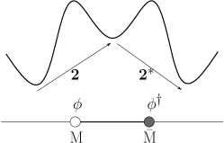
(a)

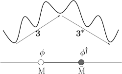
(b)

Figure 1: A schematic illustration of the nonperturbative potential and kinks interpolating between the ground state and the metastable states, in the cases of (a) $N_{c}=2$ and (b) $N_{c}=3$. Kinks ($\phi$ and $\phi^{{\dagger}}$) can be identified with monopoles ($M$ and $\bar{M}$) from the bulk $3+1$ dimensional point of view. The total configuration is a bound state of a monopole and an antimonopole.

Let us discuss the representations of these objects. The fields $\phi$ and $\phi^{{\dagger}}$ in the effective theory transform as ${\bf N_{c}}$ and ${\bf N_{c}}^{*}$ (anti)fundamental representations under $\text{SU}(N_{c})$, respectively. The degrees of freedom of $\phi$ is $2(N_{c}-1)$ after fixing $\text{U}(1)_{D}$ gauge symmetry. For instance $\phi={1\over\sqrt{1+|b_{1}|^{2}}}(1,b_{1})^{T}$ for $N_{c}=2$, and $\phi={1\over\sqrt{1+|b_{1}|^{2}+|b_{2}|^{2}}}(1,b_{1},b_{2})^{T}$ for $N_{c}=3$. For $N_{c}=2$, $\phi$ ($\phi^{{\dagger}}$) represents one (anti)kink, as can be seen in Fig. 1(a). Each of them corresponds to one (anti)monopole in the bulk. For $N_{c}=3$, which is the case of the CFL phase, one (anti)monopole is a composite state of $N_{c}-1=2$ (anti)kinks, each of which has one complex moduli (position and phase), as seen in Fig. 1(b).

We conclude that (anti)monopoles belong to ${\bf N_{c}}$ (${\bf N_{c}}^{*}$) fundamental representations of $\text{SU}(N_{c})$, and they appear as a mesonic bound state. This mesonic bound state belong to ${\bf N_{c}}\otimes{\bf N_{c}}^{*}={\bf 1}\oplus{\bf N_{c}^{2}-1}$ representation. It was shown in ZZ78 that the singlet in this decomposition does not appear in the spectrum in the ${\mathbb{C}}P^{1}$ model ($N_{c}=2$). This was interpreted in Markov:2004mj that the singlet corresponds to a set of monopole and antimonopole with opposite charges, which is unstable to decay. Although there is no such a calculation for $N_{c}\geq 3$, we expect that the same holds.

Before closing this subsection, let us make one comment on fermions. As discussed in W78 ; D'Adda:1978kp , fermions can be incorporated to the ${\mathbb{C}}P^{N_{c}-1}$ model. In fact, quasiparticles of quarks are shown to be trapped in the core of non-Abelian vortices in Yasui:2010yw , in which fermion zero modes belonging to the triplet of the $\text{SU}(2)$ unbroken symmetry in the core of the vortex have been found. However coupling to the bosonic ${\mathbb{C}}P^{2}$ model is not known yet.

In summary, we found a mesonic bound state of confined monopoles with the mass $M$ given in Eq. (62) induced by the quantum effects inside a non-Abelian vortex.

IV.2 A possible quark-monopole duality

Phases	Hadron phase (hyper nuclear matter)	Color-flavor locked phase
	Confinement	Higgs
Quarks	Confined	Condensed
Monopoles	Condensed?	Confined
Coupling constant	Strong	Weak
Order parameters	Chiral condensate $\langle\bar{q}q\rangle$	Diquark condensate $\langle qq\rangle$
Symmetry breaking patterns	$\text{SU}(3)_{L}\times\text{SU}(3)_{R}\times\text{U}(1)_{B}$	$\text{SU}(3)_{C}\times\text{SU}(3)_{L}\times\text{SU}(3)_{R}\times\text{U}(1)_{B}$
	$\rightarrow\text{SU}(3)_{L+R}$	$\rightarrow\text{SU}(3)_{C+L+R}$
Fermions	Octet baryons	Octet + singlet quarks
Vectors	Octet + singlet vector mesons	Octet gluons
Nambu-Goldstone modes	Octet pions ($\bar{q}q$)	Octet + singlet pions ($\bar{q}\bar{q}qq$)
	$H$ boson	$H$ boson

Table 1: Comparisons of the physics between the hadron phase and the CFL phase in massless three-flavor QCD: symmetry breaking patterns [the $\text{U}(1)_{A}$ and discrete symmetries are suppressed here] and the elementary excitations. We have shown that confined monopoles appear in the form of the mesonic bound state in the CFL phase. Still one missing piece in the table is the properties of monopoles in the hadron phase, for which we speculate the condensation of monopoles corresponding to the condensation of quarks in the CFL phase. See the text for further explanations.

In this subsection, we would like to ask the implications of our results. In Sec. IV.1, we found the color-octet mesonic bound states formed by of monopole-antimonopole pairs. Because of the color-flavor locking, they also form flavor-octet under the remaining $\text{SU}(3)_{C+F}$. Clearly, these bound states resemble the flavor-octet mesons formed by quark-antiquark pairs in the hadron phase. This leads us to speculate on the idea of the “quark-monopole duality”: the roles played by quarks and monopoles are interchanged between the hadron phase and the CFL phase. If this is indeed the case, this would imply the condensation of monopoles in the hadron phase corresponding to the condensation of quarks in the CFL phase. This naturally embodies the dual superconducting scenario for the quark confinement in the hadron phase N74 .

The possible quark-monopole duality may have some relevance to the one-to-one correspondence of the physics without any phase transition between the hadron phase and the CFL phase conjectured by Schäfer and Wilczek SW99 . This is called the “hadron-quark continuity” and may be realized in the QCD phase structure in three-flavor limit as explicitly shown in HTYB06 ; YTHB07 . The correspondence in the quark-monopole duality and the hadron-quark continuity is summarized in Table 1. The idea of the hadron-quark continuity is supported by a number of nontrivial evidences: the same symmetry breaking patterns, the fact that confinement phase is indistinguishable from the Higgs phase FS79 , the one-to-one correspondence of the elementary excitations such as the baryons, vector mesons HTY08 , and pions YTHB07 , and the equivalence of the form of the partition functions in a finite volume called the $\epsilon$-regime YK09 , between the hadron phase and the CFL phase.

The quark-monopole duality raises a question regarding possible other states formed by monopoles. In the hadron (confining) phase, a baryonic bound state is made of three quarks. It has been found in Bali:2000gf by the lattice QCD simulations that three quarks are connected by a Y-shaped junction of color electric flux tubes. What is the counterpart in the CFL phase? We expect that it is a junction of three non-Abelian vortices with total color fluxes canceled out at the junction point: red, blue, and green color magnetic flux tubes meet at one point, see Fig. 2. We note that they carry correct the baryon number as we expect for a baryon; each flux tube carries the $\text{U}(1)_{B}$ winding number 1/3, and all of them join together to constitute one $\text{U}(1)_{B}$ vortex with the $\text{U}(1)_{B}$ winding number one. However we have not specified the electromagnetic charges of fluxes at this stage because we have ignored the electromagnetic coupling of vortices. A similar string junction (without monopoles) is known to exist in a $\text{U}(1)\times\text{U}(1)$ model Bevis:2008hg . The configuration in Fig. 2 cannot be discussed in the effective field theory of a single vortex anymore, but one may be able to do that by considering multivortex effective theory.

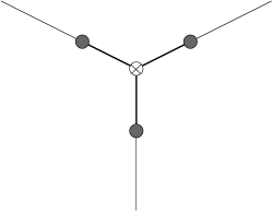
Figure 2: Baryonic bound state of three monopoles. Three monopoles are connected by a Y-shaped junction of color magnetic flux tubes with the total color canceled out. $\text{U}(1)_{B}$ vortex is represented by $\otimes$ at the junction point. This state is dual to a baryon made of three quarks connected by a Y-shaped junction of three color electric flux tubes in the hadron (confining) phase.

Finally, let us note the effect of the strange quark mass $m_{s}$ with the charge neutrality and the $\beta$-equilibrium conditions, as is expected in the physical dense matter like inside the neutron stars. This situation is considered previously without the quantum effects for the orientational modes and the nonexistence of monopoles in the CFL phase is shown ENY10 . Even if we further take into account the quantum effects, they are negligibly-small: the scale of the potential $m_{s}^{2}/g_{s}$ for the orientational modes induced by $m_{s}$ ENY10 , is much larger than that induced by the quantum effects $M^{2}$, for realistic values of the parameters, $m_{s}\sim 100\ {\rm MeV}$, $\mu\sim 500\ {\rm MeV}$, and $\Delta\sim 50\ {\rm MeV}$; confined monopoles will be washed out by $m_{s}$. Therefore, we expect that the notion of the quark-monopole duality is well-defined close to three-flavor limit. It is also a dynamical question whether the hadron-quark continuity survives when one turns on $m_{s}$; there are other candidates for the ground state at intermediate $\mu$ other than the CFL phase under the stress of $m_{s}$, such as the meson condensed phase, the crystalline Fulde-Ferrell-Larkin-Ovchinikov phase, gluon condensed phase, etc CSC .

V Conclusion and outlook

In this paper, we have analytically shown that mesonic bound states of confined monopoles appear in the color-flavor locked phase of three-flavor QCD at large quark chemical potential $\mu$. They are dynamically generated as kinks by the quantum fluctuations in the effective world-sheet theory for the orientational modes on a non-Abelian vortex. The mass of monopoles has been computed as $M\sim\Delta\exp[-c(\mu/\Delta)^{2}]$ with the superconducting gap $\Delta$ and some constant $c$.

Both of the mesonic and baryonic bound states of monopoles studied in this paper have long fluxes extending to spatial infinity. In a realistic situation these may not be appropriate because they have infinite energy. In order for them to have finite energy, such long fluxes can be made as loops, as illustrated in Fig. 3. For a meson, one can check if this can occur by studying the ${\mathbb{C}}P^{2}$ model on compactified space $S^{1}$. For a baryon the situation would be more difficult. A possible configuration for a baryon is given in Fig. 3(b).

(a)

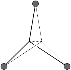
(b)

Figure 3: Illustrations of (a) a meson and (b) a baryon with finite energy. Flux tubes make loops. (a) corresponds to a vortex loop with monopole-antimonopole, which looks like a necklace. In (b) three color magnetic fluxes joint at two ends of a single $\text{U}(1)_{B}$ vortex denoted by a broken line.

Before closing the paper, let us address several important questions to be investigated in the future.

1. Although we have shown that confined monopoles dynamically appear as the monopole-antimonopole mesons by the quantum fluctuations, their topological properties are still unclear. First of all, one should clarify the homotopy group responsible for the existence or the topological stability of monopoles. One should also calculate the color magnetic charge of the confined monopoles and check if the Dirac condition for the color magnetic charge is indeed satisfied. The color magnetic flux should be related to the dynamically induced $\text{U}(1)_{D}$ gauge field. These are in contrast to the situation in the SUSY QCD: flux matching between a monopole and a vortex attached to it has been demonstrated Eto:2006dx .

2. Our derivation is based on the effective world-sheet theory on a non-Abelian vortex derived from the time-dependent Ginzburg-Landau Lagrangian. This is only valid near the critical temperature of the CFL phase. One should argue the existence of monopoles far away from the critical temperature, e.g., at $T=0$. As this concerns, the analysis beyond the Ginzburg-Landau theory can be studied by the Bogoliubov-de Genne equations which describe condensates and quasiparticles from the fermion degrees of freedom. In fact fermion modes have been studied in the presence of a non-Abelian vortex by the Bogoliubov-de Genne equations Yasui:2010yw .

3. In the case of the SUSY QCD, quantum effects in the (1+1)D on a vortex can be explained by instanton effects in the original (3+1)D theory Shifman:2004dr ; SY07 . Actually, instantons can stably exist inside the vortex world-sheet Eto:2004rz . In real QCD at asymptotic large $\mu$, bulk instanton effects with the energy $\sim 1/g_{s}^{2}\gg 1$ are highly suppressed due to the asymptotic freedom of QCD and the screening of instantons S01 . The instanton energy in the vortex world-sheet is $C_{0,3}\sim(\mu/\Delta)^{2}\gg 1/g_{s}^{2}$ [see Eq. (50)], which is further suppressed, consistent with our result. As in the SUSY QCD, the quantum effects inside the vortex may be explained by instantons trapped in it, which remains as a future problem. On the other hand, the fact that the instanton energy $C_{0,3}\sim(\mu/\Delta)^{2}$ inside the vortex is larger than the one $\sim 1/g_{s}^{2}$ in the bulk implies that instantons are repulsive from vortices.

Note added.—While this work was being completed, we learned that A. Gorsky, M. Shifman, and A. Yung GSY11 have independently found very closely related results.

References

- (1) Y. Nambu, Phys. Rev. D 10, 4262 (1974); G. ’t Hooft, in High Energy Physics, edited by A. Zichichi (Editrice Compositori, Bologna, 1976); S. Mandelstam, Phys. Rept. 23, 245 (1976).
- (2) H. Suganuma, S. Sasaki, and H. Toki, Nucl. Phys. B 435, 207 (1995).
- (3) K. I. Kondo, Phys. Rev. D 57, 7467 (1998).
- (4) N. Seiberg and E. Witten, Nucl. Phys. B 426, 19 (1994) [Erratum-ibid. B 430, 485 (1994)]; Nucl. Phys. B 431, 484 (1994).
- (5) J. Greensite, Prog. Part. Nucl. Phys. 51, 1 (2003).
- (6) M. N. Chernodub and V. I. Zakharov, Phys. Atom. Nucl. 72, 2136 (2009).
- (7) E. Shuryak, Prog. Part. Nucl. Phys. 62, 48 (2009).
- (8) M. Eto, M. Nitta, and N. Yamamoto, Phys. Rev. Lett. 104, 161601 (2010).
- (9) M. G. Alford, K. Rajagopal, and F. Wilczek, Nucl. Phys. B537, 443 (1999).
- (10) M. G. Alford, A. Schmitt, K. Rajagopal, and T. Schafer, Rev. Mod. Phys. 80, 1455 (2008).
- (11) M. M. Forbes and A. R. Zhitnitsky, Phys. Rev. D 65, 085009 (2002); K. Iida and G. Baym, Phys. Rev. D 66, 014015 (2002).
- (12) A. P. Balachandran, S. Digal, and T. Matsuura, Phys. Rev. D 73, 074009 (2006).
- (13) E. Nakano, M. Nitta, and T. Matsuura, Phys. Rev. D 78, 045002 (2008); Prog. Theor. Phys. Suppl. 174, 254 (2008).
- (14) D. B. Kaplan, arXiv:nucl-th/9506035.
- (15) M. Eto and M. Nitta, Phys. Rev. D 80, 125007 (2009).
- (16) M. Eto, E. Nakano, and M. Nitta, Phys. Rev. D 80, 125011 (2009).
- (17) Y. Hirono, T. Kanazawa, and M. Nitta, arXiv:1012.6042 [Phys Rev. D (to be published)].
- (18) A. Hanany and D. Tong, J. High Energy Phys. 0307 (2003) 037; R. Auzzi, S. Bolognesi, J. Evslin, K. Konishi and A. Yung, Nucl. Phys. B673, 187 (2003).
- (19) M. Shifman and A. Yung, Phys. Rev. D 70, 045004 (2004); A. Hanany and D. Tong, JHEP 0404, 066 (2004).
- (20) D. Tong, Phys. Rev. D 69, 065003 (2004); Y. Isozumi, M. Nitta, K. Ohashi, and N. Sakai, Phys. Rev. D 71, 065018 (2005); M. Eto, Y. Isozumi, M. Nitta, K. Ohashi, and N. Sakai, J. Phys. A 39, R315 (2006).
- (21) M. Shifman and A. Yung, Rev. Mod. Phys. 79, 1139 (2007).
- (22) A. Gorsky, M. Shifman, and A. Yung, Phys. Rev. D 71, 045010 (2005).
- (23) A. Gorsky, M. Shifman, and A. Yung, Phys. Rev. D 73, 065011 (2006);
- (24) T. Schäfer, Phys. Rev. D 65, 094033 (2002); N. Yamamoto, J. High Energy Phys. 12 (2008) 060.
- (25) I. Giannakis and H.-c. Ren, Phys. Rev. D 65, 054017 (2002); K. Iida and G. Baym, Phys. Rev. D 63, 074018 (2001); 66, 059903(E) (2002).
- (26) H. Abuki, Nucl. Phys. A 791, 117 (2007).
- (27) A. Schmitt, Q. Wang, and D. H. Rischke, Phys. Rev. D 66, 114010 (2002).
- (28) E. Abrahams and T. Tsuneto, Phys. Rev. 152, 416 (1966); C. A. R. Sá de Melo, M. Randeria, and J. R. Engelbrecht, Phys. Rev. Lett. 71, 3202 (1993).
- (29) I. Giannakis and H.-c. Ren, Nucl. Phys. B669, 462 (2003).
- (30) A. B. Zamolodchikov and A. B. Zamolodchikov, Annals Phys. 120, 253 (1979); Nucl. Phys. B 379 (1992) 602.
- (31) A. D’Adda, M. Lüscher, and P. Di Vecchia, Nucl. Phys. B 146, 63 (1978).
- (32) E. Witten, Nucl. Phys. B 149, 285 (1979).
- (33) E. Witten, Phys. Rev. Lett. 81, 2862 (1998).
- (34) M. A. Shifman, Phys. Rev. D 59, 021501 (1998).
- (35) V. Markov, A. Marshakov, and A. Yung, Nucl. Phys. B 709, 267 (2005).
- (36) A. D’Adda, P. Di Vecchia, and M. Lüscher, Nucl. Phys. B 152, 125 (1979).
- (37) S. Yasui, K. Itakura, and M. Nitta, Phys. Rev. D 81, 105003 (2010); arXiv:1010.3331 [cond-mat.mes-hall].
- (38) T. Schäfer and F. Wilczek, Phys. Rev. Lett. 82, 3956 (1999).
- (39) T. Hatsuda, M. Tachibana, N. Yamamoto, and G. Baym, Phys. Rev. Lett. 97, 122001 (2006).
- (40) N. Yamamoto, M. Tachibana, T. Hatsuda, and G. Baym, Phys. Rev. D 76, 074001 (2007).
- (41) E. H. Fradkin and S. H. Shenker, Phys. Rev. D 19, 3682 (1979); T. Banks and E. Rabinovici, Nucl. Phys. B 160, 349 (1979).
- (42) T. Hatsuda, M. Tachibana, and N. Yamamoto, Phys. Rev. D 78, 011501 (2008).
- (43) N. Yamamoto and T. Kanazawa, Phys. Rev. Lett. 103, 032001 (2009).
- (44) T. T. Takahashi, H. Matsufuru, Y. Nemoto, and H. Suganuma, Phys. Rev. Lett. 86, 18 (2001); T. T. Takahashi, H. Suganuma, Y. Nemoto, and H. Matsufuru, Phys. Rev. D 65, 114509 (2002).
- (45) N. Bevis and P. M. Saffin, Phys. Rev. D 78, 023503 (2008).
- (46) M. Eto, Y. Isozumi, M. Nitta, K. Ohashi, and N. Sakai, Phys. Rev. Lett. 96, 161601 (2006); R. Auzzi, M. Shifman, and A. Yung, Phys. Rev. D 73, 105012 (2006) [Erratum-ibid. D 76, 109901 (2007)]; M. Eto, K. Konishi, G. Marmorini, M. Nitta, K. Ohashi, W. Vinci, and N. Yokoi, Phys. Rev. D 74, 065021 (2006); M. Eto, K. Hashimoto, G. Marmorini, M. Nitta, K. Ohashi, and W. Vinci, Phys. Rev. Lett. 98, 091602 (2007); R. Auzzi, S. Bolognesi, and M. Shifman, Phys. Rev. D 81, 085011 (2010); M. Eto, T. Fujimori, S. Bjarke Gudnason, Y. Jiang, K. Konishi, M. Nitta, and K. Ohashi, JHEP 1011, 042 (2010).
- (47) For instance, see M. Eto et al., Nucl. Phys. B 780, 161 (2007); M. Nitta and W. Vinci, arXiv:1012.4057 [Nucl. Phys. B (to be published)].
- (48) M. Eto, Y. Isozumi, M. Nitta, K. Ohashi, and N. Sakai, Phys. Rev. D 72, 025011 (2005); T. Fujimori, M. Nitta, K. Ohta, N. Sakai, and M. Yamazaki, Phys. Rev. D 78, 105004 (2008).
- (49) A. Gorsky, M. Shifman, and A. Yung, arXiv:1101.1120 [hep-ph].