Optimal receptor-cluster size determined by intrinsic and extrinsic noise

Abstract

Biological cells sense external chemical stimuli in their environment using cell-surface receptors. To increase the sensitivity of sensing, receptors often cluster. This process occurs most noticeably in bacterial chemotaxis, a paradigm for sensing and signaling in general. While amplification of weak stimuli is useful in the absence of noise, its usefulness is less clear in the presence of extrinsic input noise and intrinsic signaling noise. Here, exemplified in a bacterial chemotaxis system, we combine the allosteric Monod-Wyman-Changeux model for signal amplification by receptor complexes with calculations of noise to study their interconnectedness. Importantly, we calculate the signal-to-noise ratio, describing the balance of beneficial and detrimental effects of clustering for the cell. Interestingly, we find that there is no advantage for the cell to build receptor complexes for noisy input stimuli in the absence of intrinsic signaling noise. However, with intrinsic noise, an optimal complex size arises in line with estimates of the size of chemoreceptor complexes in bacteria and protein aggregates in lipid rafts of eukaryotic cells.

I Introduction

Biological cells can sense and respond to various chemicals in their environment. However, the precision with which a cell can measure and internally evaluate the concentration of a specific ligand molecule is negatively affected by many sources of noise raj08 ; sha08 . There is external input noise (extrinsic noise) from the random arrival of ligand molecules at the cell-surface receptors by diffusion ber77 ; tka08 ; end08b , as well as various sources of intracellular signaling noise (intrinsic noise) due, e.g., to receptor dynamics, adaptation, and signal transduction yu08 , all relying on random chemical events. Nonetheless several biological examples exist in which measurements are performed with surprisingly high sensitivity. In bacterial chemotaxis, for instance, the bacterium Escherichia coli can respond to changes in concentration as low as 3.2 nM man03 , corresponding to only three molecules in the cell volume. High sensitivity is observed also in spatial sensing by single cell eukaryotic organisms, such as during aggregation of the social amoeba Dictyostelium discoideum haa07 and during mating of Saccharomyces cerevisiae (budding yeast) man04 . Furthermore, axon growth cones of neurons respond to an estimated change in concentration of about one molecule in the volume of the growth cone mor09 , and T cells of our immune system respond to a single peptide-major histocompatibility complex on a target cell syk96 . How can this sensitivity be understood despite the various sources of noise?

The best characterized signal-transduction pathway is the bacterial chemotaxis pathway, allowing cells to swim to sources of nutrients such as sugars and amino acids, and away from toxins ber99 . Cells are equipped with different receptor types with Tar among the most abundant receptors (hundreds to thousands of copies per cell). Tar specifically binds aspartate (or its non-metabolizable analogue MeAsp). An increase in ligand concentration, as occurring, e.g., when the cell swims towards the source of an attractant, inhibits receptor signaling activity and keeps the cell on course. In contrast, a decrease in attractant concentration, as occurring, e.g., when the cell swims in the wrong direction, increases receptor signaling activity. This enhances the probability for the cell to randomly find a new and hopefully better direction of swimming. Cells are further equipped with an adaptation mechanism, which allows them to sense changes in ligand concentration over a wide range of background concentration. Specifically, cells adapt their signaling activity by receptor methylation and demethylation. Methylation by enzyme CheR increases the receptor signaling activity, while demethylation by enzyme CheB decreases receptor activity.

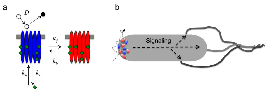
Figure 1: (color online) Schematic of bacterial cell with polar receptor cluster. (a) Receptor clusters are composed of smaller signaling complexes (here exemplified for $N=5$ receptors), which are either off/inactive (blue/left) on/active (red/right). Ligand molecules arrive at receptors by diffusion (with diffusion constant $D$) and bind/unbind. Receptor complexes randomly switch between the two states, from off to on with rate constant $k_{f}$ and from on to off with rate constant $k_{b}$. Additionally, receptors adapt by receptor methylation (rate constant $k_{R}$) and demethylation (rate constant $k_{B}$). Diamonds (green) indicate methyl-groups on receptors. (b) Shown is a trajectory of a diffusing ligand molecule, which comes on and off of the receptor cluster with $N_{C}=9$ complexes (and hence $N_{T}=N_{C}\cdot N=45$ receptors in total). The chemotaxis signaling pathway ultimately regulates the flagellated rotary motors for cell motility.

Receptor clustering is well documented in bacterial chemotaxis sou04b and is known to amplify tiny changes in ligand concentration similar to an antenna. Experimental evidence for clustering is based on structural approaches ame02 , imaging by fluorescence microscopy thi07 , including photo-activated localization microscopy (PALM) gre09 , as well as cryo-electron microscopy bri08 ; khu08 . Receptor clusters form predominantly at the cell poles as illustrated in Fig. 1, possibly due to the increased membrane curvature end09a . At a smaller scale, receptor clusters are composed of smaller signaling complexes. The notion of receptor complexes is supported by high-resolution imaging with PALM gre09 , as well as by the extracted sensitivity and cooperativity from dose-response curves (activity changes in response to ligand stimuli) measured by in vivo fluorescence resonance energy transfer (FRET). As an example, Fig. 2a shows previously published dose-response curves of the receptor activity from in vivo FRET experiments (see figure caption and end08a for details). Briefly, cells were genetically engineered to only express the Tar receptor. Different curves correspond to different modification (adaptation) states of the receptors.

To explain the dose-response data, the Monod-Wyman-Changeux (MWC) model mon65 was used to successfully describe signaling by two-state receptor complexes (Fig. 1a) sou04a ; mel05 ; key06 ; end08a . The complex size, i.e. the number of strongly coupled receptors in a complex, was estimated to be about 10-20 receptors. Alternative receptor models, later found to be inconsistent with the FRET data sko06 , are based on the Ising lattice, where moderate receptor-receptor coupling provides a mechanism for signal amplification and integration duk99 ; mel03 . Fits of the MWC model to the data are shown in Fig. 2a, which indicates an increase in complex size with receptor methylation level and hence ligand concentration (Fig. 2b). This result is consistent with the observed destabilization of polar receptor clusters by receptor demethylation or addition of attractant end09a . However, it is unknown what determines complex size.

Complex size could be limited by an imperfect physical clustering mechanism as proteins and lipids are soft materials, undergoing substantial thermal motion. Furthermore, larger complexes may not form due to the presence of other proteins in the membrane, which may constitute impurities in the receptor cluster. The dynamic aspect of receptors is supported by experiments using fluorescence recovery after photobleaching (FRAP). This indicates that receptor-cluster associated proteins, as well as components of the motors are relatively dynamic sch08 ; del09 . Alternatively, complex size might be determined by engineering principles (functionality), and hence be “optimal” for sensing. This work supports the latter view.

Fig. 3 illustrates some of the advantages and disadvantages of receptor clustering. On the one hand, more receptor cooperativity, i.e. larger complexes, amplify signals better in the absence of input noise (top panels). On the other hand, random fluctuations in ligand concentration also become amplified by the complex (bottom panels). Furthermore, the closer the proximity between receptors in a cluster, the larger the fluctuations in ligand concentration for the cell, because nearby receptor complexes measure previously bound ligand molecules due to rebinding. Hence, clustering may render complexes highly prone to noise and reduce the cell’s signal processing capabilities. Indeed, sources of noise are ubiquitous in biological sensing.

Extrinsic input noise arises from the random arrival of ligand molecules at the cell-surface receptors, constituting the fundamental physical limit on concentration sensing, derived by Berg & Purcell in 1977 ber77 and subsequently by others bia05 ; rap06 ; end08b ; end09b ; end09c . Specifically, Bialek & Setayeshgar applied the Fluctuation-Dissipation Theorem (FDT) kub66 to derive the uncertainty in ligand sensing by receptors from the fluctuations in receptor occupancy. Furthermore, if previously bound ligand molecules are removed, the uncertainty is significantly decreased end08b . Such removal prevents ligand molecules from rebinding the receptors, and hence overcounting of the same ligand molecules by the cell. A potential mechanism for ligand removal is receptor internalization, e.g. by endocytosis of ligand-bound receptors in eukaryotic cells aqu10 .

In addition to extrinsic noise, there is intrinsic noise in the signaling pathway, including the random receptor-complex switching between the on (active) and off (inactive) states (similar to flickering of ion channels), as well as random receptor methylation and demethylation events Nis10 . Since the concentrations of methylation enzyme CheR and demethylation enzyme CheB are low, i.e. about a hundred copies per cell li04 , the fluctuations in receptor methylation level are expected to be significant kor04 . To compensate for their small numbers, enzymes were found to transiently tether to the receptors. This allows them to act on groups of 6-8 receptors li05 , reducing the noise in receptor methylation level due to the larger number of available modification sites end06 . In addition to these random biochemical events, there are further downstream signaling events, ultimately the random switching of the motors between its two rotational states.

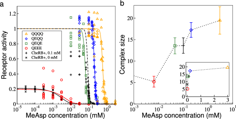
Figure 2: (color online) Data of chemotaxis signaling. (a) Dose-response curves as measured by in vivo FRET (symbols) and corresponding fits by the MWC model (solid lines) for E. coli cells expressing only Tar receptors. Cell types include adapting (CheRB+) and non-adapting, engineered cheRcheB mutants (QEEE, QEQE, QEQQ, and QQQQ with glutamate (E) or glutamine (Q) at four specific receptor modification sites). CheRB+ cells are adapted either to zero attractant (x symbols) or to 0.1 mM MeAsp (+ symbols). (b) Corresponding receptor complex sizes with 95.4% confidence intervals, as extracted from the fitted MWC model. (inset) Same on linear plot to resolve zero ambient curve. Data and model curves, fitted with Principal Component Analysis, are reproduced from end08a .

How is signaling by receptor complexes affected by extrinsic and intrinsic noise? In this work, we use the well-characterized example of bacterial chemotaxis to combine the allosteric MWC model for signaling by receptor complexes key06 ; end08a with calculations of noise to study their interconnectedness. Using the FDT kub66 ; bia05 , we calculate the uncertainty in ligand concentration sensing by the cell. Specifically, we consider the effects of the random arrival of ligand molecules at the receptors by diffusion and rebinding, switching of the receptor complexes, and receptor methylation/demethylation. While these effects have been described individually before, we combine these to address signaling by multiple receptor complexes in a cell. Based on a simplified model, we then calculate the signal-to-noise ratio (SNR), summarizing the balance of beneficial and detrimental effects of clustering for the cell. Interestingly, we find that there is no advantage for the cell to assemble receptor complexes for noisy input stimuli in the absence of intrinsic signaling noise. However, with such intrinsic noise included, an optimal complex size arises in line with estimates of the sizes of chemoreceptor complexes in bacteria and protein aggregates in eukaryotic cells.

The paper is organized as follows: In Section II we describe amplification of stimuli and extrinsic noise by receptor complexes. In section III, we derive the uncertainty in ligand concentration sensing by multiple receptor complexes in the cell. In section IV we combine the information provided in sections II and III to derive an optimal complex size, determined by the balance between signal and noise amplification by the receptor complexes. We conclude with final comments and discussion in section V. Furthermore, appendix A provides details on our model and, starting from the Master equation, derives the noise terms using the van Kampen expansion. Appendix B is devoted to summarizing the parameter values used. In appendix C we examine the effect of receptor distribution on the uncertainty of sensing.

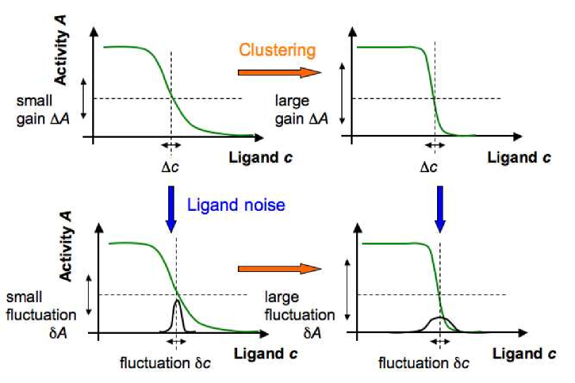
Figure 3: (color online) Schematic of dose-response curves of receptor activity. (top panels) Receptor cooperativity leads to steeper curves and hence larger amplification $\Delta A$ of a small stimulus, given by a change in ligand concentration $\Delta c$. (bottom panels) Noise in the stimulus, $\delta c$, represented by a peaked distribution, is amplified by receptor cooperativity as well, indicated by a fluctuation in activity $\delta A$. Receptor clustering, a potential side-effect of complex formation, leads to a further increase in input noise, shown by a broader distribution on the right.

II Stimulus and noise amplification

Signaling in bacterial chemotaxis is quantitatively interpreted within the MWC model. In this model, receptors form signaling complexes, believed to consist of about 10-20 receptors. Due to strong receptor-receptor coupling within a complex, a complex is an effective two-state system with all receptors either on or off together. Specifically, we consider MeAsp-binding to complexes of the Tar receptor in line with recent experiments end08a . Since MeAsp binds more favorably to the receptor off than to the receptor on state, ligand generally tends to turn the receptor activity off, whereas receptor methylation favors the on state and so compensates for ligand binding during adaptation.

In the MWC model, the probability that a receptor complex is active, i.e. the receptor activity, $A$, depends only on the free-energy difference $F$ (free energy from now on) between its on and off states key06 ; end08a

$$A=\frac{1}{1+e^{F}}$$ (1)

with energies in units of thermal energy $k_{B}T$. In this model, for a complex size of $N$ receptors, the complex free energy is simply $N$ times the free energy of a single receptor

$$F=N\left[E+\ln\left(\frac{1+c/K_{D}^{\text{off}}}{1+c/K_{D}^{\text{on}}}\right)\right]$$ (2)

with ligand concentration $c$ and ligand dissociation constants $K_{D}^{\text{on}}$ and $K_{D}^{\text{off}}$ for the on and off states, respectively. These constants represent the ligand concentrations at which the receptor in each state is occupied by ligand with 50 percent probability. In the absence of ligand, the free energy of a receptor is given by $E=\alpha-\beta\,m_{1}$ with $m_{1}$ the methylation level (methyl-group concentration) corresponding to a single receptor, and parameters $\alpha$ and $\beta$ recently determined for the Tar receptor end08a . Eq. (2) can be written in terms of the total methylation level (concentration) of the whole complex using $m=Nm_{1}$, resulting in

$$F=N\alpha-\beta m\,+\,N\ln\left(\frac{1+c/K_{D}^{\text{off}}}{1+c/K_{D}^{\text{on}}}\right).$$ (3)

This model has been very successful in describing stimulus amplification, precise adaptation to persistent stimulation, and signal integration by mixed receptor types. For instance, the MWC model is able to describe the dose-response curves in Fig. 2 end08a and other data key06 ; sko06 ; end07 .

In cells adapted to average steady-state activity $\bar{A}$, the methylation level $\bar{m}$ is determined by precise adaptation to ligand concentration $\bar{c}$ via

$$\bar{m}=\frac{1}{\beta}\left[N\alpha-\ln(1/\bar{A}-1)-N\ln\left(\frac{1+\bar{c}/K_{D}^{\text{on}}}{1+\bar{c}/K_{D}^{\text{off}}}\right)\right].$$ (4)

The mechanism for the cell to achieve precise adaptation was originally proposed by Barkai & Leibler bar97 and was later identified as integral feedback control yi00 . Briefly, if the dynamics of the methylation level are independent of the available modification sites and external ligand concentration, then the adapted steady-state activity only depends on cell-specific parameters. Specifically, the dynamics of adaptation were recently determined cla10

$$\frac{dm}{dt}=k_{R}(1-A)-k_{B}A^{3},$$ (5)

where $k_{R}$ ($k_{B}$) is the rate constant of methylation (demethylation) by enzymes CheR (CheB). Eq. (5) assumes that CheR only methylates active receptors and CheB only demethylates inactive receptors in line with experimental observation. Furthermore, for demethylation CheB needs to be activated by phosphorylation and may act cooperatively with other CheB enzymes, explaining the $A^{3}$ dependence in Eq. (5) cla10 .

For initially adapted cells, signal amplification is obtained by expanding the activity in terms of a small stimulus $\Delta c$. In the linear regime, the change in receptor-complex activity is given by

$$\Delta A=\left(\frac{\partial A}{\partial F}\right)\left(\frac{\partial F}{\partial c}\right)\Delta c=-N\bar{A}(1-\bar{A})\Delta n\frac{\Delta c}{\bar{c}}$$ (6)

with $\partial A/\partial F=-\bar{A}(1-\bar{A})$, $\partial F/\partial c=N\Delta n/\bar{c}$, and

$$\Delta n=\frac{\bar{c}}{\bar{c}+K_{D}^{\text{off}}}-\frac{\bar{c}}{\bar{c}+K_{D}^{\text{on}}}$$ (7)

the difference in receptor occupancy between its on and off states. Hence, due to receptor cooperativity in the MWC model the response $\Delta A$ corresponds to an amplification of small stimuli by complex size $N$. For larger stimuli, the response $\Delta A$ saturates to zero or maximal activity (Fig. 3, top panels), which occurs when the associated free-energy change is comparable to the thermal energy ($\Delta F\approx 1$, see Fig. 4). As a consequence, a proper investigation of signaling by receptor complexes requires the full non-linear expression for the activity in Eq. (1).

Importantly, Eq. (6) also applies to amplification of ligand noise, i.e. $\delta A\propto N\delta c$ with $\delta c$ describing a small fluctuation in ligand concentration, indicating that receptor complex formation and cooperativity also have a detrimental effect (Fig. 3, bottom panels).

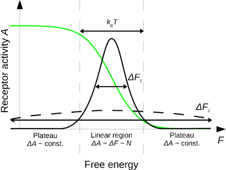
Figure 4: (color online) Activity of receptor complex $A(F)=1/(1+\exp(F))$ in green (light gray) and distribution of signaling complexes as a function of complex free energy $F$ (solid black line: small changes $\Delta F_{1}$, dashed black line: large changes $\Delta F_{2}$). Free energies in units of thermal energy $k_{B}T$, indicated by top arrow.

III Uncertainty of sensing

The uncertainty in sensing ligand concentration stems from extrinsic noise (random arrival of ligand molecules at receptors by diffusion and their rebinding), as well as intrinsic signaling noise (receptor complex switching and methylation/demethylation), projected outside the cell in form of extrinsic noise in disguise. If we neglect cross correlations (in this section for illustrative purposes), the uncertainty has the form $\langle(\delta c)^{2}\rangle_{\tau}=\sum_{k}\langle(\delta c)^{2}\rangle_{\tau}^{\text{k}}$ with contributions $k$ and $\tau$ an averaging time of the noise due to slower downstream signaling. The aim of this section is to demonstrate how the different contributions are affected by receptor complex size. Specifically, we show which contributions are amplified and which ones are not. This will help classifying noise sources more effectively, and guide the investigation of the optimal complex size in the next section.

Bialek & Setayeshgar recently calculated the uncertainty in ligand concentration using a single MWC complex as a biological measurement device bia08 . In their model, the slow (compared to ligand binding and unbinding) random switching between the on and off states of the complex leads to a release or uptake of several ($N\Delta n$) ligand molecules, since both states are characterized by different ligand dissociation constants. Here, we first extend the model by Bialek & Setayeshgar bia08 to multiple MWC complexes of Tar receptors. Subsequently, we apply the method to intrinsic methylation noise, and also discuss the other noise contributions to the uncertainty.

The dependence of the activity on the switching of the receptor complex is described by

$$\frac{dA(t)}{dt}=k_{f}[1-A(t)]-k_{b}A(t)$$ (8)

with the forward and backward rate constants given by $k_{f}$ and $k_{b}$, respectively (cf. Fig. 1a). The resulting steady-state value for the activity is given by

$$\bar{A}=\frac{k_{f}}{k_{f}+k_{b}}=\frac{1}{1+e^{\bar{F}}}$$ (9)

with

$$e^{\bar{F}}=\frac{k_{b}}{k_{f}}.$$ (10)

Now, we consider $N_{C}$ such receptor complexes, which, due to a change in receptor occupancy from switching, couple to the ligand diffusion equation

$$\!\!\!\!\!\frac{dA_{j}(t)}{dt} =k_{f}[1-A_{j}(t)]-k_{b}A_{j}(t)$$ (11a)

$$\!\!\!\!\!\frac{\partial c(\vec{x},t)}{\partial t} =D\nabla^{2}c(\vec{x},t)+N\Delta n\sum_{l=1}^{N_{C}}\delta(\vec{x}-\vec{x}_{l})\frac{dA_{l}(t)}{dt},$$ (11b)

where $A_{j}$ is the receptor-complex activity of the $j$th complex at position $\vec{x}_{j}$. Furthermore, in Eq. (11b) parameter $D$ is the diffusion constant and $\delta(\dots)$ is the Dirac delta function to describe the location of the complexes.

Following Refs. bia05 ; end09b , we linearize Eqs. (11a) and (11b) around the steady-state receptor-complex activity and ligand concentration via $\delta A=A(t)-\bar{A}$ and $\delta c(t)=c(t)-\bar{c}$, respectively. We further linearize the rate constants $\delta k_{f}(t)=k_{f}(t)-\bar{k}_{f}$ and $\delta k_{b}(t)=k_{b}(t)-\bar{k}_{b}$, allowing us to apply the FDT below bia05 . Specifically, we replace the fluctuations in rate constants by fluctuations in their conjugate variable, i.e. the receptor-complex free energy bia05 , by using

$$\delta F =\delta E+N\Delta n\frac{\delta c}{\bar{c}}$$

$$=\frac{\delta k_{b}}{\bar{k}_{b}}-\frac{\delta k_{f}}{\bar{k}_{f}},$$ (12a)

obtained by linearizing Eqs. (3) and (10).

Next, we Fourier Transform the linearized equations $d(\delta A_{j})/dt$ and $\partial(\delta c)/\partial t$ into frequency and wave-vector space, defined by $G(\vec{x},t)=\int\frac{d\omega}{2\pi}\frac{dk^{3}}{(2\pi)^{3}}\exp\{i(\vec{k}\vec{x}-\omega t)\}\hat{G}(\omega,\vec{k})$ for any integrable function $G$. This results in an equation for frequency-dependent fluctuations in the activity of the $j$-th complex

$$\!\!\!\!\!\!\!\!\!\!\!(\bar{k}_{f}+\bar{k}_{b}-i\omega)\delta\hat{A}_{j}(\omega)$$

$$\quad\quad=-\bar{k}_{b}\bar{A}_{j}\left[\delta\hat{E}_{j}+N\Delta n\frac{\delta\hat{c}(\vec{x}_{j},\omega)}{\bar{c}}\right],$$ (13)

and the wavevector and fequency-dependent variation in ligand concentration

$$\delta\hat{c}(\vec{k},\omega)=\frac{-i\omega N\Delta n}{(Dk^{2}-i\omega)}\sum_{l=1}^{N_{C}}e^{-i\vec{k}\vec{x}_{l}}\delta\hat{A}_{l}.$$ (14)

To remove the $\vec{x}$ dependence in Eq. (13), we invert the spatial Fourier Transform in Eq. (14), resulting in

$$\delta\hat{c}(\vec{x}_{j},\omega)=\frac{-i\omega N\Delta n}{\pi^{2}D}\left[\frac{1}{2a}\delta\hat{A}_{j}(\omega)+\frac{\pi}{4}\sum_{l\neq j}^{N_{C}}\frac{\delta\hat{A}_{l}(\omega)}{|\vec{x}_{j}-\vec{x}_{l}|}\right],$$ (15)

where the receptor complex dimension $a$ was introduced to regularize an integral. Eq. (15) is valid for low frequencies $\omega<\!\!<D/a^{2}$, i.e. we assume the time to read out the receptor free energy to be long compared to the correlation time between receptor-complex switching events bia08 . Inserting this equation into Eq. (13), we obtain

$$\left[\bar{k}_{f}+\bar{k}_{b}-i\omega\left(1+\bar{k}_{b}\bar{A}\frac{N^{2}\Delta n^{2}}{2\pi Da\bar{c}}\right)\right]\delta\hat{A}_{j}(\omega)$$

$$=i\omega\bar{k}_{b}\bar{A}\frac{N^{2}\Delta n^{2}}{4\pi D\bar{c}}\sum_{l\neq j}^{N_{C}}\frac{\delta\hat{A}_{l}(\omega)}{|\vec{x}_{j}-\vec{x}_{l}|}-\bar{k}_{b}\bar{A}\delta\hat{E}_{j}(\omega).$$ (16)

Next, we sum over all receptor complexes using $N_{C}\delta\hat{A}=\sum_{j=1}^{N_{C}}\delta\hat{A}_{j}$ and $\delta\hat{E}=\sum_{j=1}^{N_{C}}\delta\hat{E}_{j}$ to obtain the total receptor activity and free energy. Furthermore, we introduce the geometric structure factor $\Phi=\sum_{j\neq 1}^{N_{C}}\frac{1}{|\vec{x}_{1}-\vec{x}_{j}|}$, valid for receptor complex distributions for which each receptor complex is equivalent to all the other receptor complexes (ring or sphere of receptors) bia05 . With these quantities introduced, we obtain

$$\!\!\!\!\!\!\!\!\!N_{C}\left\{\bar{k}_{f}+\bar{k}_{b}-i\omega\left[1+\frac{\bar{k}_{b}\bar{A}N^{2}\Delta n^{2}}{2\pi D\bar{c}}\left(\frac{1}{a}+\frac{\Phi}{2}\right)\right]\right\}\delta\hat{A}$$

$$\quad\quad=-\bar{k}_{b}\bar{A}\delta\hat{E}.$$ (17)

Using the FDT, we calculate the noise power spectrum of the receptor-complex activity, defined by $\langle\delta\hat{A}(\omega)\delta\hat{A}^{*}(\omega)\rangle$, from the deterministic linear response to a small perturbation in the receptor-complex free energy

$$S_{A}(\omega)= \frac{2}{\omega}\text{Im}\left[-\frac{\delta\hat{A}}{\delta\hat{E}}\right]$$ (18a)

$$= \frac{2\bar{k}_{f}(1-\bar{A})(1+\Sigma)}{N_{C}[(\bar{k}_{f}+\bar{k}_{b})^{2}+\omega^{2}(1+\Sigma)^{2}]}$$ (18b)

$$\stackrel{{\scriptstyle\omega\rightarrow 0}}{{\longrightarrow}} \frac{2\bar{k}_{f}(1-\bar{A})(1+\Sigma)}{N_{C}(\bar{k}_{f}+\bar{k}_{b})^{2}}$$ (18c)

with $\Sigma=\frac{\bar{k}_{b}\bar{A}N^{2}\Delta n^{2}}{2\pi D\bar{c}}(1/a+\Phi/2)$ and Eq. (18c) valid in the zero-frequency limit. Note the minus sign in Eq. (18a) is introduced since a positive $\delta\hat{E}$ leads to a negative $\delta\hat{A}$ bia08 . From $\delta A=-N\bar{A}(1-\bar{A})\Delta n\frac{\delta c}{\bar{c}}$ (cf. Eq. (6)), we obtain for the time-averaged variance of the ligand concentration

$$\langle(\delta c)^{2}\rangle_{\tau}=\left[\frac{\bar{c}}{N\Delta n\bar{A}(1-\bar{A})}\right]^{2}\frac{S_{A}(0)}{\tau}$$ (19)

with $\tau$ the averaging time determined by slow, downstream signaling, and finally for the relative uncertainty in sensing

$$\frac{\langle(\delta c)^{2}\rangle_{\tau}^{\text{SR}}}{\bar{c}^{2}} = \frac{2}{N_{C}N^{2}\Delta n^{2}\bar{k}_{f}(1-\bar{A})\tau}$$ (20)

$$\quad+\frac{1}{N_{C}\pi D\bar{c}\tau}\left(\frac{1}{a}+\frac{\Phi}{2}\right).$$

The first term on the right-hand side represents the uncertainty in ligand concentration due to the release and uptake of $N\Delta n$ ligand molecules induced by the randomly switching receptor complexes (S). The second term is due to diffusion and represents the additional uncertainly from rebinding of previously bound ligand molecules (R). Due to this term, the uncertainty depends on the spatial distribution of the receptor complexes on the cell surface. Specifically, the term proportional to $1/a$ describes the rebinding of ligand molecules to the same receptor complex, while the term proportional to $\Phi$ describes the rebinding to the other receptor complexes. This latter contribution becomes the larger the smaller the proximity of the receptor complexes, e.g. in the polar receptor cluster (appendix C). Fast ligand diffusion (or removal of bound ligand molecules by an efficient cellular uptake mechanism) reduces this term aqu10 . Furthermore, in Eq. (20) the number of receptor complexes $N_{C}$ in the denominators reduces the uncertainty by spatial averaging.

The FDT method can also be used to calculate the uncertainty in ligand concentration from random receptor methylation and demethylation events. The rate of change of a small deviation of the receptor-complex activity $\delta A$ due to a change in total receptor methylation level $\delta m$ is given by

$$\frac{d(\delta A)}{dt}=\frac{\partial A}{\partial m}\frac{d(\delta m)}{dt}$$ (21)

where $dm/dt$ and $d(\delta m)/dt$ are given by Eq. (5) and its linearised version, respectively. Using

$$\delta F = \frac{\delta k_{R}}{\bar{A}(\bar{k}_{R}+3\bar{k}_{B}\bar{A}^{2})}$$ (22)

$$\quad+\frac{\bar{A}^{2}}{1-\bar{A}}\cdot\frac{\delta k_{B}}{\bar{k}_{R}+3\bar{k}_{B}\bar{A}^{2}},$$

linearization and Fourier transformation finally leads to the relative uncertainty in ligand concentration

$$\frac{\langle(\delta c)^{2}\rangle_{\tau}^{\text{MR}}}{\bar{c}^{2}} = \frac{2}{N_{C}U^{2}\Delta n^{2}\bar{k}_{R}(1-\bar{A})\tau}$$ (23)

$$\quad+\frac{1}{N_{C}\pi D\bar{c}\tau}\left(\frac{1}{a}+\frac{\Phi}{2}\right),$$

where the first term on the right hand side describes the contribution from random receptor methylation and demethylation events (M), respectively leading to a release and take-up of ligand molecules. This term is inversely proportial to $N^{2}$, and hence, is not amplified by receptor cooperativity (cf. Eq. (6)) in analogy to the intrinsic ligand noise arising from random switching of the receptor complex in Eq. (20). The second term in Eq. (23) is idential to Eq. (20) and describes the contribution from diffusion (R), as released and taken up ligand molecules lead to additional uncertainty in ligand concentration.

So far the contribution to the uncertainty from random binding and unbinding of ligand molecules (L) to the receptor complex is still missing. To avoid the complexity of different rates for the on and off states, we assume diffusion-limited binding to the receptor cluster and write for the additional uncertainty end09b ; aqu10

$$\frac{\langle(\delta c)^{2}\rangle_{\tau}^{\text{L}}}{\bar{c}^{2}}=\frac{1}{4\pi DR_{s}\bar{c}\tau},$$ (24)

calculated from Poisson statistics and the diffusive flux to an absorbing sphere of radius $R_{s}$, which represents the dimension of the receptor cluster. Eq. (24) is considered the fundamental physical limit of sensing as it cannot be reduced by any intracellular sensing mechanism. This extrinsic noise is amplified due to the absence of a $N^{2}$ factor in the denominator.

In summary, intrinsic and extrinsic noise affect the uncertainty of sensing differently, i.e. only extrinsic noise is amplified. In the next section, we consider an integrative model of extrinsic ligand noise and intrinsic noise from receptor methylation/demethylation noise. The receptor-complex switching noise is much smaller due to the large switching rates and hence is assumed to be averaged out. By using the receptor activity of the whole cell as a read-out of signaling, we are able to compare the properties of stimulus and noise transmission.

IV Optimal receptor complex size

What effects have stimulus and noise amplification on the signaling capabilities of the whole cell, and specifically, is there an optimal complex size? In the cell, we assume a large receptor cluster of $N_{\text{T}}$ identical receptors divided into $N_{C}$ smaller receptor signaling complexes of $N$ Tar receptors each (see Fig. 1b). We now calculate the $N$-dependent SNR for the total activity $A_{T}$ of the cell in response to a uniform, non-saturating stimulus $\Delta c\propto\bar{c}$

$$\text{SNR}=\frac{\text{Signal}}{\text{Noise}}=\frac{<\Delta A_{\text{T}}>_{N}^{2}}{<\!\!<\delta A_{\text{T}}^{2}>\!\!>_{N}},$$ (25)

where the Signal is defined by the squared-mean response of all receptors in the cell $<\!\!\Delta A_{\text{T}}\!\!>_{N}^{2}=\langle\sum_{i}^{N_{T}}\Delta A_{i}\rangle^{2}=(N_{T}\langle\Delta A\rangle)^{2}$ to the stimulus, neglecting cross-correlations between the activities of different complexes. In contrast, the Noise is expressed by the mean-square deviation of the independently fluctuating receptor complexes $<\!\!<\delta A_{\text{T}}^{2}>\!\!>_{N}=\sum_{j}^{N_{C}}\langle\delta A_{j}^{2}\rangle=N_{C}\langle\delta A^{2}\rangle$. Since measurements are not done instantaneously by the cell, we use time-averaged activities $\langle...\rangle=\tau^{-1}\int_{t}^{t+\tau}....d\tilde{t}$. This leads to the following general expressions for the Signal and the Noise

$$<\Delta A_{\text{T}}>_{N}^{2} = \left\{\frac{N_{\text{T}}}{\tau}\int_{t}^{t+\tau}\left[A(F(c(\tilde{t})+\Delta c,m(\tilde{t}))-A(F(c(\tilde{t}),m(\tilde{t}))\right]\,d\tilde{t}\right\}^{2}$$ (26)

$$<\!\!<\delta A_{\text{T}}^{2}>\!\!>_{N} = \frac{N_{\text{C}}}{\tau}\int_{t}^{t+\tau}[N\,A(F(c(\tilde{t}),m(\tilde{t})))-N\,\bar{A}]^{2}\,d\tilde{t}=\frac{N_{\text{T}}N}{\tau}\int_{t}^{t+\tau}[A(F(c(\tilde{t}),m(\tilde{t})))-\bar{A}]^{2}\,d\tilde{t}$$ (27)

with $A=A(F)$ the receptor complex activity, depending on ligand concentration $c$ and methylation level $m$ via the free energy $F=F(c,m)$. Both ligand concentration $c=c(\tilde{t})$ and methylation level $m=m(\tilde{t})$ depend on time. Further note that the factor $N$ on the right-hand side of Eq. (27) appears as each receptor in a complex has the same activity. Even though the stimulus and noise (included below) are small, Eqs. (26) and (27) allow for non-linear effects in the activity for the large complexes sizes considered.

For computational feasibility, we exploit the ergodic hypothesis, allowing us to replace the time averages by the ensemble averages. This leads to the respective Signal and Noise

$$<\Delta A_{\text{T}}>_{N}^{2} = \left\{N_{\text{T}}\int\left[A(F(c+\Delta c,m))-A(F(c,m))\right]\,P(c,m)\,dc\,dm\right\}^{2}$$ (28)

$$<\!\!<\delta A_{\text{T}}^{2}>\!\!>_{N} = N_{\text{T}}N\int[\,A(F(c,m))-\,\bar{A}]^{2}\,P(c,m)\,dc\,dm.$$ (29)

In the Signal, receptor complexes experience a stimulus $\Delta c$ on top of a fluctuating ligand concentration, while in the Noise, fluctuations in activity are measured relative to the average activity. In Eqs. (28) and (29), we further use a bivariate Normal distribution to describe the joint probability of the ligand concentration and methylation level at a receptor complex, given by

$$P(c,m)=\frac{e^{-\frac{1}{2(1-\rho^{2})}\left[\frac{(c-\bar{c})^{2}}{\langle(\delta c)^{2}\rangle}+\frac{(m-\bar{m})^{2}}{\langle(\delta m)^{2}\rangle}-\frac{2\rho(c-\bar{c})(m-\bar{m})}{\sqrt{\langle(\delta c)^{2}\rangle}\sqrt{\langle(\delta m)^{2}\rangle}}\right]}}{2\pi\sqrt{\langle(\delta c)^{2}\rangle}\sqrt{\langle(\delta m)^{2}\rangle}\sqrt{1-\rho^{2}}}.$$ (30)

In addition to the variances $\langle(\delta c)^{2}\rangle$ and $\langle(\delta m)^{2}\rangle$, Eq. (30) also depends on covariance $\langle(\delta c)(\delta m)\rangle$, included in the correlation coefficient $\rho=\langle(\delta c)(\delta m)\rangle/[\sqrt{\langle(\delta c)^{2}\rangle}\sqrt{\langle(\delta m)^{2}\rangle}]$. While the methylation level can fluctuate due to random methylation and demethylation events independent from fluctuations in ligand concentration, fluctuations in ligand concentration can induce fluctuations in the methylation level due to adaptation (via parameter $\rho$).

To calculate the variances and covariance we use a simplified Master equation, describing how the receptor-complex activity depends on external ligand concentration and receptor methylation level. The ligand noise includes effects of the random arrival of ligand molecules at the receptors and their rebinding by diffusion, given by rate $k_{d}=D/a^{2}$. We then apply the van Kampen expansion to obtain the second moments of the joint distribution (see appendix A for details).

IV.1 Ligand noise

First, we only consider extrinsic ligand noise by setting the methylation level $m(\tilde{t})$ equal to the constant adapted value $\bar{m}$. The distribution of the ligand concentration is now effectively given by $P(c)=1/\sqrt{2\pi\langle(\delta c)^{2}\rangle}\exp\{-(c-\bar{c})^{2}/[2\langle(\delta c)^{2}\rangle]\}$, assumed to be Normal with average ligand concentration $\bar{c}$ and variance

$$\langle(\delta c)^{2}\rangle=\frac{\bar{c}}{a^{3}}$$ (31)

(see appendix A for more details).

Importantly, the Signal and Noise have characteristic $N$-dependencies, which need to be examined in order to answer the question of the optimal complex size. We first consider the linear regime of the activity, as this can be solved analytically. In this case, Eqs. (28) and (29) reduce to

$$<\!\Delta A_{\text{T}}\!>_{N}^{2}=N_{\text{T}}^{2}\left(\frac{\partial A}{\partial c}\right)^{2}\Delta c^{2}\propto N^{2},$$ (32)

and

$$<\!\!<\delta A_{\text{T}}^{2}>\!\!>_{N}=N_{\text{T}}N\left(\frac{\partial A}{\partial c}\right)^{2}\langle(\delta c)^{2}\rangle\propto N^{3},$$ (33)

using Eq. (6). As a result, the SNR scales as $N^{-1}$ and hence decreases for increasing complex size. This indicates that a single receptor is better than a complex of multiple receptors for signaling due to the more rapid increase of the Noise with complex size than the Signal. Note also that the SNR is proportional to the total number of receptors $N_{T}$ in a cell.

In order to consider the full non-linear activity of the receptors, we numerically integrate Eqs. (28) and (29) with $m$ set to $\bar{m}$ and $P(c)$ instead of $P(c,m)$. Fig. 5 shows contour plots of the Signal, Noise, and SNR as a function of complex size and ligand concentration. In Fig. 6, the scaling behavior is confirmed by plotting the three quantities for three different ligand concentrations as a function of complex size.

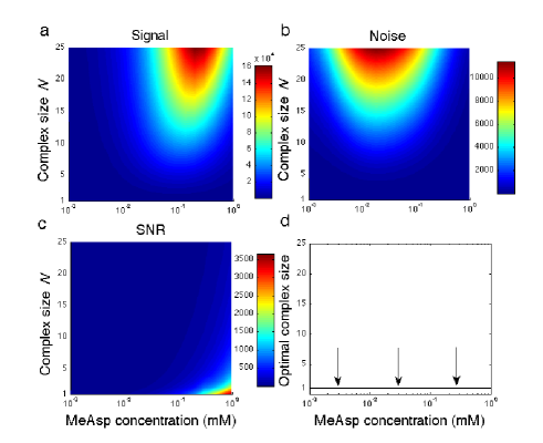
Figure 5: (color online) Absence of an optimal complex size for extrinsic ligand noise. (a) Signal, (b) Noise, and (c) SNR as a function of MeAsp concentration and complex size, i.e. the number of Tar receptors in a complex. (d) There is no maximum of the SNR for complex sizes larger than one receptor. For each MeAsp concentration, the same non-saturating MeAsp stimulus is applied to all complex sizes. Parameter values are given in appendix B. Integration performed with the quadrature method in Matlab (Mathworks, Natwick, MA).

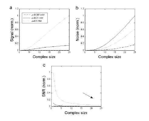
Figure 6: Numerical confirmation of scaling behavior for extrinsic ligand noise. (a) Signal, (b) Noise, and (c) SNR from Fig. 5 as a function of complex size for three different MeAsp concentrations $0.001$, $0.01$, and $0.1$ mM. Curves in each panel are normalized by their maximal value.

IV.2 Ligand and methylation noise

Next, we include additional fluctuations in the receptor methylation concentration, as explicitly described by Eqs. (28), (29), and (30). The variance of the methylation level is given by

$$\langle(\delta m)^{2}\rangle = \frac{1}{\beta(3-2\bar{A})a^{3}}$$ (34)

$$\!\!\!\!\!\!\!\!\!\!\!\!\!\!\!\!\!\!\!\!\!\!\!+\frac{k_{R}(3-2\bar{A})(1-\bar{A})(\Delta nN)^{2}}{\beta[k_{d}+k_{R}(3-2\bar{A})(1-\bar{A})\beta]ca^{3}}$$

with $\beta=-\partial F/\partial m$. The first term on the right-hand side of Eq. (34) represents the intrinsic methylation noise, which is independent of complex size consistent with the amplified version of Eq. (23). The reason for this $N$-independence is that a large complex has more enzymes bound to the receptors and hence suffers from larger noise than a small complex. However, a large complex also has an increased relaxation rate $k_{R}+3k_{B}\bar{A}^{2}$, restoring the average methylation level more quickly. The second term on the right-hand side of Eq. (34) is the ligand-induced methylation noise with its characteristic $N^{2}$-dependence due to amplification by the receptors in the complex.

Furthermore, the covariance between the ligand concentration and methylation level is given by

$$\langle(\delta c)(\delta m)\rangle=\frac{k_{R}(3-2\bar{A})(1-\bar{A})\Delta nN}{k_{d}+k_{R}(3-2\bar{A})(1-\bar{A})\beta}.$$ (35)

Together with the variances, this equation allows the calculation of the previously mentioned correlation coefficient $\rho$. Its value is zero if fluctuations in methylation level are independent of fluctuations in ligand concentration, and one if there are no ligand-independent fluctuations in the methylation level. In our model, the correlation coefficient turns out to be rather small, i.e. no larger than 0.0001 for the parameter values used.

To check the validity of the small-noise approximation, we compare the intrinsic methylation noise from the analytical calculation (first term on the right-hand side of Eq. (34)) with simulations of the Master equation using the exact Gillespie algorithm gil77 . (Note the methylation noise is significantly larger than the ligand noise and hence is used for this test.) Specifically, the algorithm requires two random numbers. The first determines whether to methylate the complex with rate $k_{R}[1-A(M)]$ or whether to demethylate with rate $k_{B}A(M)^{3}$, where $M=a^{3}m$ is the current methylation level (the dependence on the constant external ligand concentration $\bar{c}$ is not shown). The second, $R$, is needed to correctly increment the simulation time. $R$ is chosen with a uniform probability on the interval $[0,1]$, and the time is increased according to $\delta t=1/\{[k_{R}(1-A(M))+k_{B}A(M)^{3}]\ln(1/R)\}$. Using parameters from appendix B and concentrations ranging from $10^{-3}$ to $1$ mM, Fig. 7 shows indeed that the two approaches deliver very similar distributions for the methylation level.

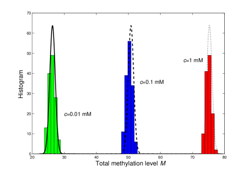
Figure 7: (color online) Comparison of the intrinsic methylation noise from the small-noise approximation (van Kampen expansion) with Gillespie simulations of the Master equation. Shown are histograms of methylation level from simulations for external ligand concentrations $c=0.01$ mM (green/left), $c=0.1$ mM (blue/middle), and $c=1$ mM (red/right). Also shown are corresponding Normal distributions with variance given by Eq. (38), drawn with solid, dashed, and dotted lines, respectively.

We next consider how the cell’s Signal and the Noise scale with complex size. First, in the linear activity regime the Signal is again given by Eq. (32). Analoguous to the case with ligand noise only, the receptor complex is able to fully amplify the stimulus. (The only difference is that the Signal is saturated by the stimulus or noise at smaller complex sizes due to the noise contribution from methylation/demethylation.) In contrast, the Noise has a new regime in the presence of additional noise from methylation/demethylation

$$<\!\!<\delta A_{\text{T}}^{2}>\!\!>_{N} \propto N\left[\langle(\delta A)^{2}\rangle_{m}+\langle(\delta A)^{2}\rangle_{c}\right]$$ (36)

$$\propto N(const+N^{2}).$$

For small complex sizes, the ligand-induced $N$-dependent activity noise can be neglected with respect to the constant contribution from methylation/demethylation, leading to scaling with $N$. For larger complex sizes, the Noise scales as $N^{3}$. The two regimes lead to an optimal complex size, since the SNR, now given by

$$\text{SNR}\propto N_{T}\frac{N}{const+N^{2}},$$ (37)

first increases proportional to $N$ and then decreases as $N^{-1}$. Hence, the intrinsic noise from methylation/demethylation introduces a noise floor, below which it is advantageous for the cell to increase the complex size. However, once amplified ligand noise becomes comparable to the noise floor for large complexes, the Noise increases more rapidly than the Signal with further increasing complex size.

To address the behavior for the non-linear activity, Figs. 8 and 9 show the results from the numerical evaluation of the double integrals in Eqs. (28) and (29), confirming our analysis of the scaling. For large complex sizes, deviations from the linear regime can be observed. The shape of the optimal complex-size curve as a function of ligand concentration is ultimately determined by the functional dependence of $\Delta n$ on $\bar{c}$ (Eq. (7)), which describes the sensitivity of the receptor occupancy to changes in ligand concentration.

IV.3 Methylation noise

Finally, we consider the case of only intrinsic noise from fluctuations in the methylation level. Eq. (30) effectively reduces to the Normal distribution $P(m)=1/\sqrt{2\pi\langle(\delta m)^{2}\rangle}\exp\{-(m-\bar{m})^{2}/[2\langle(\delta m)^{2}\rangle]\}$ with average methylation level $\bar{m}$ and variance

$$\langle(\delta m)^{2}\rangle=\frac{1}{\beta(3-2\bar{A})a^{3}},$$ (38)

corresponding to the first term in Eq. (34). In Eqs. (28) and (29), the ligand concentration is set to the average value $\bar{c}$.

Similar to the previous two cases, the Signal behaves as Eq. (32), i.e. scales as $N^{2}$ due to stimulus amplification in the linear activity regime. (However, since the methylation/demethylation noise is independent of complex size, only the stimulus and not the noise can saturate the Signal for large complex sizes.) The Noise scales as $N$ from the prefactor in Eq. (29) since the methylation/demethylation noise is independent of complex size. As a result, the SNR is proportional to the complex size. Hence, large complexes are always better for signaling than small complexes (provided the amplified stimulus is not saturating the Signal). This analysis is confirmed by numerical integration in Figs. 10 and 11.

In summary, intrinsic and extrinsic noise have profoundly different effects on sensing. Only in the presence of both does an optimal complex size emerge. This result is intuitively clear. Amplification of extrinsic noise is worse than amplification of the stimulus as receptor complexes behave incoherently for noise amplification and become fewer in number for increasing complex size. However, amplification of extrinsic noise is acceptable as long as it stays below the intrinsic noise and does not saturate receptor activity. Only when the amplified extrinsic noise becomes larger than the intrinsic noise does its effect become detrimental.

V Discussion

Here we investigated the conditions under which an optimal receptor complex size emerges in order to provide a potential explanation for the observed receptor cooperativity (Fig. 2) and complexes sizes as imaged by high-resolution microscopy gre09 . Specifically, we considered the signal-to-noise ratio (SNR), i.e. the ratio between the Signal in response to a small stimulus in ligand concentration and the Noise from random fluctuations of the activity, based on all the receptor complexes in a cell. Using the MWC model for signaling by receptor complexes, we include amplification of both stimulus and extrinsic ligand noise, as well as the effects of intrinsic noise from random receptor methylation/demethylation. Also included are correlations between the ligand and methylation/demethylation noise, since fluctuations in ligand concentration can induce an adaptational response and hence fluctuations in methylation level. Note, however, that very slow fluctuations in ligand concentration are fully removed by perfect adaptation.

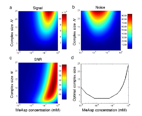
Figure 8: (color online) Optimal complex size in the presence of both extrinsic ligand and intrinsic methylation noise. (a) Signal, (b) Noise, and (c) SNR as a function of ligand concentration and complex size of Tar receptors. (d) There is a maximum of the SNR at complex sizes larger than one receptor. Parameter values are given in appendix B.

By setting up the Master equation and applying the small-noise approximation, we found that only including extrinsic ligand noise leads to a decrease in SNR with complex size as the Noise inceases more rapidly with complex size than the Signal. When instead only considering intrinsic noise, there is no penalty for the cell to make larger and larger complexes, and the SNR increases with increasing complex size. However, including both noise sources introduces a complex size-independent noise floor from the intrinsic noise. Hence, an increase in complex size is beneficial until the amplified and hence size-dependent extrinsic noise increases beyond the noise floor. An optimal complex size for complexes with more than one receptor is the consequence (Figs. 8 and 9).

Extrinsic ligand noise results from the random binding, as well as rebinding of previously measured ligand molecules. Importantly, the latter contribution depends on the distribution of the receptors. In particular, the smaller the complex-complex proximity in clusters the larger the increase in uncertainty in sensing ligand concentration. For ligand diffusion in aqueous solution, the effect of rebinding is generally negligible (appendix C). A ligand molecule just released from a receptor is quickly removed by diffusion, hence preventing it from rebinding. However, diffusion can be much slower in biologically relevant circumstances. For instance, in E. coil chemoreceptors are localized in the inner membrane, which is surrounded by the dense, viscous periplasm, separating the inner and outer cell membranes. Here, the ligand diffusion constant can be a thousand times smaller bra86 and rebinding of previously bound ligand molecules could be significant.

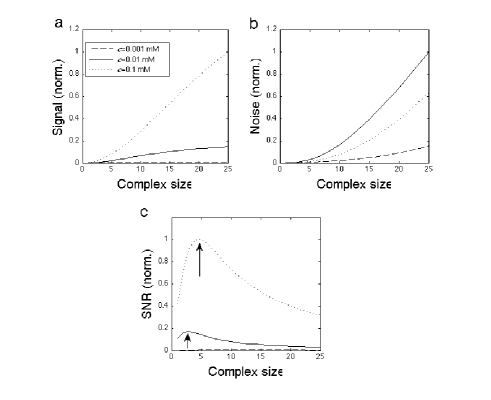
Figure 9: Numerical confirmation of scaling behavior in the presence of both extrinsic ligand and intrinsic methylation noise. (a) Signal, (b) Noise, and (c) SNR from Fig. 8 as a function of complex size for three different MeAsp concentrations $0.001$, $0.01$, and $0.1$ mM. Curves in each panel are normalized by their maximal value.

As demonstrated recently, the detrimental effect of ligand rebinding can be reduced by internalization of ligand-bound receptors, such as frequently occurs in eukaryotic cells aqu10 . Receptor internalization effectively turns the cell into an absorber of ligand molecules, which increases the accuracy of sensing end08b ; aqu10 . While chemoreceptors in bacteria are not internalized, transporters for uptake of sugars and amino acids could colocalize with the receptors to simulate the effect of internalization. Specifically, the uptake of sugars and amino acids is mainly conducted by periplasmic permeases, which are ABC-like transporters hed94 . The best studied permease is the maltose system in E. coli. Maltose enters the outer membrane through the LamB pores. Subsequently, it is sensed by either directly binding the Tar receptor, or maltose-binding protein MalE, which is then either bound by the Tar receptor for sensing or by the permease for transport of maltose into the cell. Additional work will be required to better understand the role of the periplasm in the accuracy of sensing.

While our model is able to explain the observed complex sizes from FRET data, there are a number of simplifying model assumptions. First, we calculated the Signal and Noise at the receptor level, neglecting downstream signaling events such as phosphorylation and dephosphorylation reactions. However, such reactions are known to be very fast, $50-1000\,\text{s}^{-1}$ cla10 , and hence their noise is quickly averaged out by the motor. Second, for our calculation of the noise to be computationally feasible, we assume diffusion-limited binding to avoid difficulties with the two different receptor complex states. Third, fast intrinsic noise from random receptor switching between its two activity states is assumed to be averaged out and hence is also neglected.

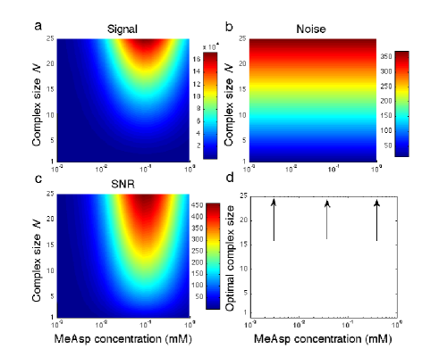
Figure 10: (color online) Absence of optimal complex size for intrinsic methylation noise only. (a) Signal, (b) Noise, and (c) SNR as a function of ligand concentration and complex size of Tar receptors. (d) There is no maximum of the SNR since the SNR keeps increasing for increasing complex size. Parameter values are given in appendix B.

A remaining question is if optimization principles hold for cellular subsystems (here receptor sensing). There might be tradeoffs, potentially leading to suboptimal solutions for parts of the cell. Furthermore, receptor sensing is not the final cell’s output (here swimming), on which natural selection may operate. However, as receptors enable cells to gather information about their environment and information can only be lost, not gained during signal transduction, it appears to be a reasonable assumption to conserve this information as much as possible (if energy and resources are not limiting). To instead optimize chemotaxis signaling at the level of cell swimming, not only swimming up typical gradients, but also staying on top of gradients (at the maximum concentration) cla05 and the dynamics of gradients cel10 would need to be considered.

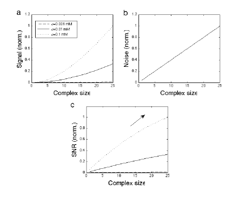
Figure 11: Numerical confirmation of scaling behavior for intrinsic methylation noise. (a) Signal, (b) Noise, and (c) SNR from Fig. 10 as a function of complex size for three different MeAsp concentrations $0.001$, $0.01$, and $0.1$ mM. Curves in each panel are normalized by their maximal value.

Our model can readily be extended from Tar-only receptor complexes to mixed complexes of multiple receptor types key06 . If ligand binds specifically to one receptor type only, the receptor fraction of each type in a mixed complex should be optimal in size with specifics depending on the ligand dissociation constants only. Furthermore, our work may be applicable to other receptors as well. While receptor clustering may be restricted to receptors with high sensing accuracy, most well-characterized sensory receptors are believed to cluster (or to oligomerize). These include the eukaryotic B-cell, T-cell, Fc$\gamma$, synaptic, as well as G-protein-coupled and ryanodine receptors ceb10 . Specifically, T-cell receptors form micro-clusters of 7-30 receptors lil10 . Such receptor aggregates are often associated with lipid rafts, islands of specific lipids with particular affinity for certain membrane proteins. Interestingly, lipid rafts were found to be small, containing mostly about 6-12 proteins gur09 and were recently even observed in bacteria lop10 . Our work may indicate that this number represents an optimal size for signal amplification, where size is restricted by extrinsic and intrinsic noise.

Appendix A Derivation of noise terms using $\Omega$ expansion

In this appendix, we set up the Master equation of the simplified problem of a receptor complex, whose activity is determined by the external ligand concentration and receptor methylation level. The dynamics of the latter are determined by adaptation. To solve for the first and second moments of the joint probability distribution from the Master equation, we apply van Kampen’s $\Omega$ expansion, where $\Omega$ is the reaction volume, allowing one to introduce a large expansion parameter kam07 . We neglect fast processes such as receptor-complex switching between different activity states and ligand-receptor binding/unbinding. Note that we use a slighly different notation in this appendix, more suitable for stochastic processes.

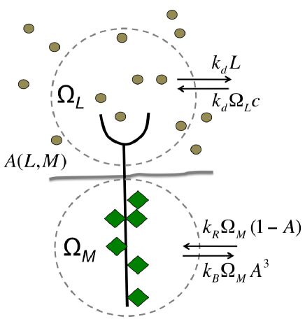
Figure 12: (color online) Simple model of receptor-complex activity $A(L,M)$ with its dependence on ligand molecules $L$ in its vicinity (volume $\Omega_{L}$) and receptor-methylation level $M$ (in volume $\Omega_{M}$). Rate constants $k_{d}$, $k_{R}$, and $k_{B}$ describe ligand diffusion with average ligand concentration $c$, methylation, and demethylation, respectively.

As shown in Fig. 12 we consider a system composed of two parts. The cell external volume $\Omega_{L}$ contains the number of ligand molecules $L$ in the vicinity of the receptor complex, which increases from $L\rightarrow L+1$ with rate $k_{d}\Omega_{L}\bar{c}$ and decreases from $L\rightarrow L-1$ with rate $k_{d}L$. The cell internal volume $\Omega_{M}$ contains the methyl-groups on the receptor, which increase from $M\rightarrow M+1$ with rate $k_{R}\Omega_{M}[1-A(L,M)]$ and decrease from $M\rightarrow M-1$ with rate $k_{B}\Omega_{M}[A(L,M)]^{3}$ (cf. macroscopic Eq. (5)). The corresponding Master equation for these one-step processes is given by

$$\frac{\partial P(L,M,t)}{\partial t}=k_{d}\Omega_{L}cP(L-1,M,t)$$

$$+k_{d}(L+1)P(L+1,M,t)$$

$$+k_{R}[1-A(L,M-1)]P(L,M-1,t)$$

$$+k_{B}[A(L,M+1)]^{3}P(L,M+1,t)$$

$$-\{k_{d}(L+\Omega_{L}c)+k_{R}[1-A(L,M)]$$

$$+k_{B}[A(L,M)]^{3}\}P(L,M,t).$$ (39)

We now define the following separation of $L$ and $M$ into macroscopic parts $c$ and $m$ of respective sizes $\Omega_{L}$ and $\Omega_{M}$, and fluctuating parts $\zeta$ and $\eta$ of respective sizes $\Omega_{L}^{1/2}$ and $\Omega_{M}^{1/2}$,

$$L(t)=\Omega_{L}c(t)+\Omega_{L}^{1/2}\zeta(t)$$ (40a)

$$M(t)=\Omega_{M}m(t)+\Omega_{M}^{1/2}\eta(t).$$ (40b)

We also define the step operators

$$\mathbb{E}_{L}^{+1}f(L)=f(L+1)$$ (41a)

$$\mathbb{E}_{L}^{-1}f(L)=f(L-1)$$ (41b)

$$\mathbb{E}_{M}^{+1}f(M)=f(M+1)$$ (41c)

$$\mathbb{E}_{M}^{-1}f(M)=f(M-1)$$ (41d)

for any arbitrary function $f(...)$. Using Eqs. 40a and 40b, in the limits of large $\Omega_{L}$ and $\Omega_{M}$, the step operators adopt the differential form kam07

$$\mathbb{E}_{L}^{\pm 1}=1\pm\Omega_{L}^{-1/2}\frac{\partial}{\partial\zeta}+\frac{1}{2}\Omega_{L}^{-1}\frac{\partial^{2}}{\partial\zeta^{2}}\pm....$$ (42a)

$$\mathbb{E}_{M}^{\pm 1}=1\pm\Omega_{M}^{-1/2}\frac{\partial}{\partial\eta}+\frac{1}{2}\Omega_{L}^{-1}\frac{\partial^{2}}{\partial\eta^{2}}\pm....$$ (42b)

with higher-order terms neglected. Transforming from the old variables $L$ and $M$ to the new variables $\zeta$ and $\eta$, we have the relations

$$P(L,M,t)\rightarrow\Pi(\zeta,\eta,t)$$ (43a)

$$\Omega_{L}^{1/2}\frac{\partial}{\partial L}P(L,M,t)=\frac{\partial}{\partial\zeta}\Pi(\zeta,\eta,t)$$ (43b)

$$\Omega_{M}^{1/2}\frac{\partial}{\partial M}P(L,M,t)=\frac{\partial}{\partial\eta}\Pi(\zeta,\eta,t).$$ (43c)

With the above relations, we transform the Master equation, now written with step operators,

$$\frac{\partial P(L,M,t)}{\partial t}=k_{d}\Omega_{L}c(\mathbb{E}_{L}^{-1}-1)P(L,M,t)$$

$$\qquad+k_{d}(\mathbb{E}_{L}^{+1}-1)LP(L,M,t)$$

$$+k_{R}\Omega_{M}(\mathbb{E}_{M}^{-1}-1)[1-A(L,M)]P(L,M,t)$$

$$+k_{B}\Omega_{M}(\mathbb{E}_{M}^{+1}-1)[A(L,M)]^{3}P(L,M,t)$$ (44)

into

$$\frac{\partial\Pi}{\partial t}-\Omega_{L}^{1/2}\frac{dc}{dt}\frac{\partial\Pi}{\partial\zeta}-\Omega_{M}^{1/2}\frac{dm}{dt}\frac{\partial\Pi}{\partial\eta}$$ (45)

$$= \!\!\!k_{d}\Omega_{L}^{1/2}c\!\!\left[-\frac{\partial}{\partial\zeta}+\frac{1}{2}\Omega_{L}^{-1/2}\frac{\partial^{2}}{\partial\zeta^{2}}\right]\!\!\Pi(\zeta,\eta,t)$$

$$+ \!\!\!k_{d}\Omega_{L}^{1/2}\left[\frac{\partial}{\partial\zeta}+\frac{1}{2}\Omega_{L}^{-1/2}\frac{\partial^{2}}{\partial\zeta^{2}}\right](c+\Omega_{L}^{-1/2}\zeta)\Pi(\zeta,\eta,t)$$

$$+ \!\!\!k_{R}\Omega_{M}^{1/2}\left[-\frac{\partial}{\partial\eta}+\frac{1}{2}\Omega_{M}^{-1/2}\frac{\partial^{2}}{\partial\eta^{2}}\right]$$

$$\qquad\qquad\cdot[1-A(c,\zeta,m,\eta)]\Pi(\zeta,\eta,t)$$

$$+ \!\!\!k_{B}\Omega_{M}^{1/2}\left[\frac{\partial}{\partial\eta}+\frac{1}{2}\Omega_{M}^{-1/2}\frac{\partial^{2}}{\partial\eta^{2}}\right]$$

$$\qquad\qquad\cdot[A(c,\zeta,m,\eta)]^{3}\Pi(\zeta,\eta,t).$$

Next we expand the receptor activity to extract its $\Omega$ dependencies using $(A+\delta A)^{3}=A^{3}+3A^{2}\delta A+O(\delta A^{2})$ with $\delta A$ a small deviation from activity $A$, and

$$A(c,\zeta,m,\eta)\approx A(c,m)+\frac{\partial A}{\partial m}\Omega_{M}^{-1/2}\eta+\frac{\partial A}{\partial c}\Omega_{L}^{-1/2}\zeta+\dots$$ (46)

Putting everything together, the terms proportional to $\Omega_{L}^{1/2}$ produce the macroscopic equation $dc/dt=0$, which indicates that the ligand concentration $c$ is already at steady state, and the terms proportional to $\Omega_{M}^{1/2}$ produce $dm/dt=k_{R}(1-A)-k_{B}A^{3}$ (cf. Eq. (5)).

Importantly, from Eq. (45) it is possible to derive equations for the mean value of the fluctuations as well as for the correlations of these fluctuations. Assuming $\Omega_{L}=\Omega_{M}=\Omega$, we first collect all the terms proportional to $\Omega^{0}$ in Eq. (45), which yields

$$\frac{\partial\Pi}{\partial t}=k_{d}\left[c\frac{\partial^{2}}{\partial\zeta^{2}}+\frac{\partial}{\partial\zeta}\zeta\right]\Pi$$

$$+\frac{1}{2}\left\{k_{R}[1-A(c,m)]+k_{B}[A(c,m)]^{3}\right\}\frac{\partial^{2}\Pi}{\partial\eta^{2}}$$

$$+k_{R}\left\{\frac{\partial A}{\partial m}+\left[\frac{\partial A}{\partial c}\zeta+\frac{\partial A}{\partial m}\eta\right]\frac{\partial}{\partial\eta}\right\}\Pi$$

$$\!\!\!\!\!\!\!\!\!\!+3k_{B}[A(c,m)]^{2}\left\{\frac{\partial A}{\partial m}+\left[\frac{\partial A}{\partial c}\zeta+\frac{\partial A}{\partial m}\eta\right]\frac{\partial}{\partial\eta}\right\}\Pi.$$ (47)

Next, multiplying by $\zeta$ and integrating over $\zeta$ and $\eta$ (using intergation by parts), produces

$$\frac{\partial\langle\zeta\rangle}{\partial t}=-k_{d}\langle\zeta\rangle.$$ (48)

The analoguous procedure for $\eta$ produces

$$\frac{\partial\langle\eta\rangle}{\partial t}=-(k_{R}+3k_{B}A^{2})\left[\frac{\partial A}{\partial m}\langle\eta\rangle+\frac{\partial A}{\partial c}\langle\zeta\rangle\right].$$ (49)

Furthermore, multiplying Eq. (47) by $\zeta^{2}$, $\eta^{2}$, and $\zeta\eta$ with subsequent integration yields, respectively,

$$\frac{\partial\langle\zeta^{2}\rangle}{\partial t} = -2k_{d}\langle\zeta^{2}\rangle+2k_{d}c$$ (50)

$$\frac{\partial\langle\eta^{2}\rangle}{\partial t} = k_{R}(1-A)+k_{B}A^{3}$$ (51)

$$-2\left(k_{R}+3k_{B}A^{2}\right)\frac{\partial A}{\partial m}\langle\eta^{2}\rangle$$

$$-2(k_{R}+3k_{B}A^{2})\frac{\partial A}{\partial c}\langle\zeta\eta\rangle$$

$$\frac{\partial\langle\zeta\eta\rangle}{\partial t} = -\left[k_{d}+\left(k_{R}+3k_{B}A^{2}\right)\frac{\partial A}{\partial m}\right]\langle\zeta\eta\rangle$$ (52)

$$-(k_{R}+3k_{B}A^{2})\frac{\partial A}{\partial c}\langle\zeta^{2}\rangle.$$

At steady state, we finally obtain

$$\langle\zeta^{2}\rangle_{s} = c$$ (53)

$$\langle\eta^{2}\rangle_{s} = \frac{1}{\beta(3-2\bar{A})}$$ (54)

$$\!\!\!\!\!\!\!\!\!\!\!\!\!\!+\frac{k_{R}(3-2\bar{A})(1-\bar{A})(\Delta nN)^{2}}{[k_{d}+k_{R}(3-2\bar{A})(1-\bar{A})\beta]c\beta}$$

$$\langle\zeta\eta\rangle_{s} = \frac{k_{R}(3-2\bar{A})(1-\bar{A})\Delta nN}{k_{d}+k_{R}(3-2\bar{A})(1-\bar{A})\beta}$$ (55)

with their characteristic $N$-dependencies, $\bar{A}$ the adapted steady-state activity, and $\Delta n$ and $\beta$ defined in Sec. II. The corresponding quantities expressed in the original variables, i.e. $\langle(\delta L)^{2}\rangle$, $\langle(\delta M)^{2}\rangle$, and $\langle(\delta L)(\delta M)\rangle$ are produced by multiplication of Eqs. 53-55 with $\Omega$. For instance, $\langle(\delta L)^{2}\rangle=\langle L\rangle$, or $\langle(\delta c)^{2}\rangle=c/\Omega\sim c/(a^{3})$ with $a$ the dimension of volume $\Omega$, is indicative of a simple Poisson process and describes the instantaneous, total fluctuations in ligand concentration.

Appendix B Parameter values

Here we provide the parameter values used for the results from section IV, presented in Figs. 5-11: $a=100$nm (dimension of receptor complex) bri08 ; khu08 , $\beta=a^{3}/2$ (energy contribution per methyl group to receptor free energy) end08a , $k_{R}a^{3}=0.1\,\text{s}^{-1}$ and $k_{B}a^{3}=2.2\,\text{s}^{-1}$ (methylation and demethylation rates) end06 ; cla10 , $\bar{A}=1/3$ (resulting adapted complex activity), $k_{f}=10^{3}\,\text{s}^{-1}$ and $k_{b}=2\cdot 10^{3}\,\text{s}^{-1}$ (rates for complex switching) shar04 , $D=300\,\mu\text{m}^{2}/\text{s}$ (diffusion constant for molecules in aqueous solution)end08b , $N_{T}=3000$ (number of receptors per cell) haz08 , $K_{D}^{\text{on}}=0.5$mM and $K_{D}^{\text{off}}=0.02$mM (MeAsp dissociation constants for Tar in the on and off states) key06 .

Appendix C Effect of receptor distribution on uncertainty

To estimate the magnitude of the structure factor $\Phi$ in Eqs. (20) and (23), and hence the importance of ligand rebinding to the uncertainty of sensing ligand concentration, we apply the following algorithm for uniformely distributing $N_{C}$ points (complexes) on a sphere. The algorithm divides the sphere in $N_{C}$ parallels and places a point on each parallel at positions given by the following equations in spherical coordinates saf97

$$h_{k} =-1+2(k-1)/(N_{C}-1)\;\;\;\;1\leq k\leq N_{C}$$ (56a)

$$\theta_{k} =\arccos{h_{k}}$$ (56b)

$$\phi_{k} =\left(\phi_{k-1}+\frac{3.6}{\sqrt{N_{C}}}\frac{1}{\sqrt{1-h_{k}}}\right)(\text{mod}\,2\pi).$$ (56c)

The number 3.6 in the algorithm can, in principle, be adjusted appropriately for the application at hand but derives essentially from best packing algorithms. The simple algorithm adopted here distributes the points spirally around the sphere and gives a good results in accordance with more sophisticated algorithms based on energy minimization between point charges on the sphere or best packing criteria, as long as $N_{C}>100$ and $N_{C}<12000$.

To represent the polar receptor cluster, we choose a small sphere of radius $R_{S}=75$nm khu08 . As a result, the structure factor for the small sphere is given by $\Phi_{S}=4.77\cdot 10^{9}\text{m}^{-1}$. In contrast, to represent receptor complexes evenly distributed over the cell surface, we use a large sphere of radius $R_{L}=1.2\,\mu$m, which leads to a smaller structure factor given by $\Phi_{L}=5.73\cdot 10^{8}\text{m}^{-1}$. Compared to rebinding to the same receptor, which is proportional to $1/a=10^{7}$m^-1 in Eq. (20), the polar receptor cluster can significantly worsen the uncertainty of sensing. However, for fast ligand diffusion in aqueous solution, the rebinding terms are negligible compared to the other contributions to the uncertainty.

References

- (1) A. Raj and A. van Oudenaarden, Cell 135, 216 (2008).
- (2) V. Shahrezaei and P.S. Swain, Curr. Opin. Biotech. 19, 369 (2008).
- (3) H.C. Berg and E.M. Purcell EM, Biophys. J. 20, 193 (1977).
- (4) G. Tkacik, T. Gregor, and W. Bialek, PLoS One 3, e2774 (2008).
- (5) R.G. Endres, N.S. Wingreen, Proc. Natl. Acad. Sci. USA 105, 15749 (2008).
- (6) R. C. Yu et al., Nature 456, 755 (2008).
- (7) H. Mao, P.S. Cremer, M.D. Manson, Proc. Natl. Acad. Sci. USA 100, 5449 (2003).
- (8) P.J.M. van Haastert, M. Postma, Biophys. J. 93, 1787 (2007).
- (9) C.L. Manahan, P.A. Iglesias, Y. Long, and P.N. Devreotes, Annu. Rev. Cell. Dev. Biol. 20, 223 (2004).
- (10) D. Mortimer et al. Proc. Natl. Acad. Sci. USA 106, 10296 (2009).
- (11) Y. Sykulev et al. Immunity 4, 565 (1996).
- (12) H.C. Berg, Physics Today 53, 24 (1999).
- (13) V. Sourjik V, Trends Microbiol. 12, 569 (2004).
- (14) P. Ames, C.A. Studdert, R.H. Reiser, and J.S. Parkinson, Proc. Natl. Acad. Sci. USA. 99, 7060 (2002).
- (15) S. Thiem, D. Kentner and V. Sourjik, EMBO J. 26, 1615 (2007).
- (16) D. Greenfield, A.L. McEvoy, H. Shroff, G.E. Crooks, N.S. Wingreen, E. Betzig, and J. Liphardt, PLoS Biol. 7, e1000137 (2009).
- (17) A. Briegel, H.J. Ding, Z. Li, J. Werner, Z. Gitai, D.P. Dias, R.B. Jensen, and G. Jensen, Mol. Microbiol. 69, 30 (2008).
- (18) C.M. Khursigara, X. Wu, and S. Subramaniam, J. Bacteriol. 190, 6805 (2008).
- (19) R.G. Endres, Biophys. J. 96, 453 (2009).
- (20) R.G. Endres, O. Oleksiuk, C.H. Hansen, Y. Meir, V. Sourjik, and N.S. Wingreen, Mol. Syst. Biol. 4, 211 (2008).
- (21) J. Monod, J. Wyman, J.P. Changeux, J. Mol. Biol. 12, 88 (1965).
- (22) V. Sourjik and H.C. Berg, Nature 428, 437 (2004).
- (23) B.A. Mello and Y. Tu, Proc. Natl. Acad. Sci. USA 102, 17354 (2005).
- (24) J.E. Keymer, R.G. Endres, M. Skoge, Y. Meir, and N.S. Wingreen, Proc. Natl. Acad. Sci. USA 103, 1786 (2006).
- (25) M.L. Skoge, R.G. Endres, N.S. Wingreen, Biophys. J. 90, 4317 (2006).
- (26) T.A.J. Duke and D. Bray, Proc. Natl. Acad. Sci. USA 96, 10104 (1999).
- (27) B.A. Mello and Y. Tu, Proc. Natl. Acad. Sci. USA 100, 8223 (2003).
- (28) S. Schulmeister, M. Ruttorf, S. Thiem, D. Kentner, D. Lebiedz, V. Sourjik, Proc. Natl. Acad. Sci. USA 105, 6403 (2008).
- (29) N. Delalez, J. Armitage, Mol. Microbiol. 71, 807 (2009).
- (30) W. Bialek and S. Setayeshgar, Proc. Natl. Acad. Sci. USA 102, 10040 (2005).
- (31) R.G. Endres and N.S. Wingreen, Prog. Biophys. Mol. Biol. 100, 33 (2009).
- (32) R.G. Endres and N.S. Wingreen, Phys. Rev. Lett. 103, 158101.
- (33) W. Rappel and H. Levine, Phys. Rev. Lett. 100, 228101 (2008).
- (34) R. Kubo, Rep. Prog. Phys. 29, 255 (1966).
- (35) G. Aquino and R.G. Endres, Phys. Rev. E. 81, 021909 (2010).
- (36) M. Nishikawa and T. Shibata, PLoS One 5, e11224 (2010).
- (37) M. Li and G.L. Hazelbauer, J. Bacteriol. 186, 3687 (2004).
- (38) E. Korobkova, T. Emonet, J.M. Vilar, T.S. Shimizu, and P. Cluzel, Nature 428, 574 (2004).
- (39) M. Li and G.L. Hazelbauer, Mol. Microbiol. 56, 1617 (2005).
- (40) R.G. Endres and N.S. Wingreen, Proc. Natl. Acad. Sci. USA 103, 13040 (2006).
- (41) R.G. Endres, J.J. Falke, and N.S. Wingreen, PLoS Comput. Biol. 3, e150 (2007).
- (42) N. Barkai and S. Leibler, Nature 387, 913 (1997).
- (43) T. Yi, Y. Huang, M.I. Simon, and J. Doyle, Proc. Natl. Acad. Sci. USA 97, 4649 (2000).
- (44) D. Clausznitzer, L. Lovdok, O. Oleksiuk, V. Sourjik, and R.G. Endres, PLoS Comp.Biol. 6: e1000784.
- (45) W. Bialek, S. Setayeshgar, Phys. Rev. Lett. 100, 258101 (2008).
- (46) D. T. Gillespie, J. Phys. Chem. 81, 2340 (1977).
- (47) J.M. Brass et al., J. Bacteriol. 165, 787 (1986).
- (48) M.A. Hediger, J. Exp. Biol. 196, 15 (1994).
- (49) D.A. Clark and L.C. Grant, Proc. Natl. Acad. Sci. USA 102, 9150 (2005).
- (50) A. Celani and M. Vergassola, Proc. Natl. Acad. Sci. USA 107, 1391 (2010).
- (51) M. Cebecauer, M. Spitaler, A. Serge, and A.I. Magee, J. Cell Sci. 123, 309 (2010).
- (52) B.F. Lillemeier, M.A. Mörtelmaier, M.B. Forstner, J.B. Huppa, J.T. Groves, M.M. Davis, Nat. Immunol. 11, 90 (2010).
- (53) T. Gurry, O. Kahramanoğullari, R.G. Endres, PLoS One 4, e6148 (2009).
- (54) D. López and R. Kolter, Genes Dev. 24, 1893 (2010).
- (55) N.G. van Kampen, Stochastic processes in physics and chemistry (Elsevier, Amsterdam, 3rd edition, 2007).
- (56) P. Sharma P, R. Varma, R.C. Sarasij, Ira, K. Gousset, G. Krishnamoorthy, M. Rao, S. Mayor, Cell 116, 577 (2004).
- (57) G.L. Hazelbauer, J.J. Falke, J.S. Parkinson, Trends Biochem. Sci. 33, 9 (2008).
- (58) E. B. Saff and A. B. J. Kuijlaars, Math. Intell. 19, 5 (1997).