Small components in $k$-nearest neighbour graphs

Abstract

Let $G=G_{n,k}$ denote the graph formed by placing points in a square of area $n$ according to a Poisson process of density 1 and joining each point to its $k$ nearest neighbours. In [2] Balister, Bollobás, Sarkar and Walters proved that if $k<0.3043\log n$ then the probability that $G$ is connected tends to 0, whereas if $k>0.5139\log n$ then the probability that $G$ is connected tends to 1.

We prove that, around the threshold for connectivity, all vertices near the boundary of the square are part of the (unique) giant component. This shows that arguments about the connectivity of $G$ do not need to consider ‘boundary’ effects.

We also improve the upper bound for the threshold for connectivity of $G$ to $k=0.4125\log n$.

1 Introduction

Let $S_{n}$ denote a $\sqrt{n}\times\sqrt{n}$ square and let $G_{n,k}$ denote the graph formed by placing points in $S_{n}$ according to a Poisson process ${\mathcal{P}}$ of density 1 and joining each point to its $k$-nearest neighbours by an undirected edge. Since we shall be interested in the asymptotic behaviour of this graph as $n\to\infty$, it is convenient to introduce one piece of notation. For a graph property $\Pi$ we say that $G_{n,k}$ has $\Pi$ with high probability (abbreviated to whp) if $\mathbb{P}(G_{n,k}\text{ has $\Pi$})\to 1$ as $n\to\infty$.

Xue and Kumar [5] proved that the threshold for connectivity is $\Theta(\log n)$; more precisely they showed that if $k=k(n)>5.1774\log n$ then $G_{n,k}$ is connected whp, and if $k=k(n)<0.074\log n$ then $G_{n,k}$ is whp not connected.

Subsequent work by Balister, Bollobás, Sarkar and Walters [2] substantially improved the upper and lower bounds to $0.5139\log n$ and $0.3043\log n$ respectively. In their proof they also showed that for any $k=\Theta(\log n)$ the graph consists of a giant component containing a proportion $1-o(1)$ of all vertices and (possibly) some other ‘small’ components of (Euclidean) diameter $O(\sqrt{\log n})$ (for a formal statement see Lemma 3).

Moreover, they showed that if $k>0.311\log n$ then $G$ has no small component within distance $O(\sqrt{\log n})$ of the boundary of $S_{n}$. Unfortunately, there is a gap between this bound and the lower bound of $0.3043$ mentioned above. This means that close to the threshold for connectivity the obstruction to connectivity could occur near the boundary of the square or it could occur in the centre (their methods did rule out the possibility that the obstruction occurs in the corner of the square). This has caused several problems in later papers (e.g., [3]) where the authors had to consider both cases in their proofs.

Our main result is the following theorem showing that, in fact, the obstruction must occur away from the boundary of $S_{n}$. This should simplify subsequent work in the area as only central components need to be considered. (Of course, the improvement itself is only of minor interest, it is the fact that the new upper bound for the existence of components near the boundary is smaller than the general lower bound that is of importance.)

Theorem 1.

Suppose that $G=G_{n,k}$ for some $k>0.272\log n$. Then there is a constant $\varepsilon>0$ such that the probability that there exists a vertex within distance $\log n$ of the boundary of $S_{n}$ that is not contained in the giant component is $O(n^{-\varepsilon})$.

Remark.

The distance $\log n$ to the boundary is much larger than the typical edge length and (non-giant) component sizes which are $O(\sqrt{\log n})$. Moreover, the theorem would still be true with $\log n$ replaced by a small power of $n$.

Our second result is the following improvement on the upper bound for connectivity of $G$.

Theorem 2.

Suppose that $G=G_{n,k}$ for some $k>0.4125\log n$. Then whp $G$ is connected.

To illustrate Theorem 2 let $D$ be a disc of radius $r$ and consider the event that there are $k+1$ points inside $D$ and no points in $3D\setminus D$ (where $3D$ denotes the disc with same centre as $D$ and three times the radius). If this event occurs then the $k$-nearest neighbours of any point in $D$ also lie in $D$: in particular, there are no ‘out’-edges from $D$ to the rest of the graph. If we choose $r$ such that $9\pi r^{2}\approx k+1$ (to maximise the probability of this event) then the probability of a specific instance of this event is about $9^{-(k+1)}$. Since we can fit $\Theta(n/\log n)$ disjoint copies of this event into $S_{n}$ we see that if $k<(\frac{1}{\log 9}-\varepsilon)\log n$ (for some $\varepsilon>0$) then whp this event occurs somewhere in $S_{n}$ and thus that $G$ has a subgraph with no out-degree. Since $1/\log 9\approx 0.455>0.4125$, Theorem 2 shows that there is a range of $k$ for which the graph is connected whp but contains pieces with no outdegree. (The corresponding result for in-degree was proved in [2].)

The proofs of these two theorems are broadly similar: they use the ideas from [2] but also consider points which are near the small component but not contained in it. Indeed, if one looks at the lower bound proved in [2] we see that the density of points near the small component is higher than average. This is an unlikely event and we incorporate it into our bounds. Indeed, the above observation that there are small pieces of the graph with no out-degree shows that any proof of Theorem 2 (or any stronger bound) must consider points outside of a potential small component and show that they send edges in.

The key step is to split into two regimes depending on whether there is a point ‘close’ to the small component. If there is no such point then the ‘excluded area’ from the small component is quite large (which is unlikely), whereas if there is such a point then it must have a small $k$-nearest neighbour radius (which is also unlikely).

2 Notation and Preliminaries

We start with some notation. For any point $x$ and real number $r$ let $D(x,r)$ denote the closed disc of radius $r$ about $x$. We shall also use the term half-disc of radius $r$ based at $x$ to mean one of the four regions obtained by dividing the disc $D(x,r)$ in half vertically or horizontally.

For a set $A$ in $S_{n}$ let $|A|$ denote the measure of $A$, and $\#A$ denote the number of points of ${\mathcal{P}}$ in $A$. For any real number $r$ let $A_{(r)}$ be the $r$-blowup of $A$ defined by

$$A_{(r)}=\{x\in\mathbb{R}^{2}:d(x,A)<r\}.$$

Note that we do allow $A_{(r)}$ to contain points outside of $S_{n}$.

Finally, whenever we use the term diameter we shall always mean the Euclidean diameter: we do not use graph diameter at any point in the paper.

We shall need a few results from the paper of Balister, Bollobás, Sarkar and Walters [2]. Since our notation is slightly different we quote them here for convenience. The first is a slight variant of Lemma 6 of [2] which follows immediately from the proof given there (see also Lemma 1 of [3]).

Lemma 3.

For fixed $c>0$ and $L$, there exists $c_{1}=c_{1}(c,L)>0$, depending only on $c$ and $L$, such that for any $k\geq c\log n$, the probability that $G_{n,k}$ contains two components each of $($Euclidean$)$ diameter at least $c_{1}\sqrt{\log n}$, is $O(n^{-L})$.

The second bounds the probability of a small component near one side, or two sides of $S_{n}$; it is explicit in the proof of Theorem 7 of [2]. (Note, Theorem 1 improves the first of these bounds.)

Lemma 4.

Suppose that $k=\Theta(\log n)$. The probability that there is a small component containing a vertex within $\log n$ of one boundary of $S_{n}$ is $O(n^{\frac{1}{2}+o(1)}5^{-k})$ and the probability that there is a small component containing a vertex within $\log n$ of two sides of $S_{n}$ is $O(n^{o(1)}3^{-k})$.

The final result follows easily from concentration results for the Poisson distribution (see e.g. [1]) and most of it is implicit in Lemma 2 of [2].

Lemma 5.

For any fixed $c$ and $L$ there is a constant $c_{2}(c,L)$ such that for any $k$ with $c\log n<k<\log n$ the probability that there is any edge of length at least $c_{2}\sqrt{\log n}$, or any two points within distance $\frac{1}{c_{2}}\sqrt{\log n}$ of each other not joined by an edge, or a point $x\in{\mathcal{P}}$ with a half-disc of radius $c_{2}\sqrt{\log n}$ based at $x$ contained entirely inside $S_{n}$ that contains no points of ${\mathcal{P}}$, is $O(n^{-L})$.

We will use the following simple but technical lemma several times.

Lemma 6.

Suppose that $A,B,C$ are three sets in $S_{n}$ with $|A|\leq|C|$ and $|B|\leq|C|$ then

$$\mathbb{P}(\text{$\#A\geq k$, $\#B\geq k$, $\#(A\cap B)=0$ and $\#C=0$})\leq\left(\frac{4|A||B|}{(|A|+|B|+|C|)^{2}}\right)^{k}.$$

Proof.

Let $A^{\prime}=(A\setminus B)\setminus C$, $B^{\prime}=(B\setminus A)\setminus C$, $C^{\prime}=C\cup(A\cap B)$, and $U=A\cup B\cup C=A^{\prime}\cup B^{\prime}\cup C$. We see that $A^{\prime},B^{\prime}$ and $C^{\prime}$ are pairwise disjoint so $|U|=|A^{\prime}|+|B^{\prime}|+|C^{\prime}|$ and, since $\#(A\cap B)=0$, that $\#A^{\prime}\geq k$, $\#B^{\prime}\geq k$. We have

$$\mathbb{P}(\#A\geq k ,\ \#B\geq k,\ \#(A\cap B)=0\text{ and }\#C=0)$$

$$=\mathbb{P}(\#A^{\prime}\geq k,\ \#B^{\prime}\geq k\text{ and }\#C^{\prime}=0)$$

$$=\sum_{l\geq k,m\geq k}\mathbb{P}(\#A^{\prime}=l,\ \#B^{\prime}=m\text{ and }\#U=l+m)$$

$$=\sum_{l\geq k,m\geq k}\mathbb{P}(\#A^{\prime}=l,\ \#B^{\prime}=m\ |\ \#U=l+m)\mathbb{P}(\#U=l+m)$$

$$\leq\max_{l\geq k,m\geq k}\mathbb{P}(\#A^{\prime}=l,\ \#B^{\prime}=m\ |\ \#U=l+m)$$

(the final line follows since $\sum_{l\geq k,m\geq k}\mathbb{P}(\#U=l+m)\leq 1$).

We have $|A^{\prime}|\leq|A|\leq|C|\leq|C^{\prime}|$ so $|A^{\prime}|\leq\frac{1}{2}|U|$ and similarly $B^{\prime}\leq\frac{1}{2}|U|$. Hence, for $l,m\geq k$,

$$\mathbb{P}(\#A^{\prime}=l,\ \#B^{\prime}=m\ |\ \#U=l+m)= \binom{l+m}{l}\left(\frac{|A^{\prime}|}{|U|}\right)^{l}\left(\frac{|B^{\prime}|}{|U|}\right)^{m}$$

$$\leq 2^{l+m}\left(\frac{|A^{\prime}|}{|U|}\right)^{l}\left(\frac{|B^{\prime}|}{|U|}\right)^{m}$$

$$\leq 2^{2k}\left(\frac{|A^{\prime}|}{|U|}\right)^{k}\left(\frac{|B^{\prime}|}{|U|}\right)^{k}$$

$$=\left(\frac{4|A^{\prime}||B^{\prime}|}{|U|^{2}}\right)^{k}$$

$$=\left(\frac{4|A^{\prime}||B^{\prime}|}{(|A^{\prime}|+|B^{\prime}|+|C^{\prime}|)^{2}}\right)^{k}.$$

Finally, observe that $|A^{\prime}|\leq|A|\leq|C|\leq|C^{\prime}|$ and $|B^{\prime}|\leq|B|\leq|C|\leq|C^{\prime}|$ imply that

$$\frac{4|A^{\prime}||B^{\prime}|}{(|A^{\prime}|+|B^{\prime}|+|C^{\prime}|)^{2}} \leq\frac{4|A||B^{\prime}|}{(|A|+|B^{\prime}|+|C^{\prime}|)^{2}}$$

$$\leq\frac{4|A||B|}{(|A|+|B|+|C^{\prime}|)^{2}}$$

$$\leq\frac{4|A||B|}{(|A|+|B|+|C|)^{2}}.$$

which completes the proof.∎

3 Proof of Theorem 2

By hypothesis we have $k>0.4125\log n$. Also, we may assume that $k<0.6\log n$ since we already know that $G_{n,k}$ is connected whp if $k\geq 0.6\log n$. Let $c^{\prime}=\max\{c_{1}(0.25,1),c_{2}(0.25,1),1\}$ be as given by Lemmas 3 and 5 and let $M=20000c^{\prime}$. (We shall reuse some of the bounds we prove here in the proof of Theorem 1 so these are convenient values.) Tile $S_{n}$ with small squares of side length $s=\sqrt{\log n}/M$. We form a graph $\widehat{G}$ on these tiles by joining two tiles whenever the distance between their centres is at most $2c^{\prime}\sqrt{\log n}$. We call a pointset ${\mathcal{P}}$ bad if any of the following hold:

1. there exist two points that are joined in $G$ but the tiles containing these points are not joined in $\widehat{G}$,

2. there exist two points, at most distance $20000s$ apart, that are not joined,

3. there exists a half-disc based at a point of ${\mathcal{P}}$ of radius $c^{\prime}\sqrt{\log n}$ that is contained entirely in $S_{n}$ and contains no (other) point of ${\mathcal{P}}$,

4. there exist two components in $G_{n,k}$ with Euclidean diameter at least $c^{\prime}\sqrt{\log n}$,

5. there exists a component of diameter at most $c^{\prime}\sqrt{\log n}$ containing a vertex within distance $2c^{\prime}\sqrt{\log n}$ of the boundary of $S_{n}$,

and good otherwise. We see that our choice of $c^{\prime}$ and $M$ together with Lemma 5 imply that the probability that any of the first three conditions occur is $O(n^{-1})$. By Lemma 3 the probability of the fourth condition is $O(n^{-1})$. Since $k>0.4125\log n>\frac{1}{\log 25}\log n$, Lemma 4 implies the probability of the last condition is $O(n^{-\varepsilon})$ for some $0<\varepsilon<1$. (Alternatively this follows from Theorem 1). Combining these we see that the probability of a bad configuration is $O(n^{-\varepsilon})$.

Suppose that ${\mathcal{P}}$ is a good configuration but $G$ is not connected. Then there exists a component $F$ with diameter at most $c^{\prime}\sqrt{\log n}$ not containing any vertex within $2c^{\prime}\sqrt{\log n}$ of the boundary of $S_{n}$. Let $A$ be the collection of tiles that contain a point of $F$. Since the configuration is good $A$ is a connected subset of $\widehat{G}$ containing no tile within $c^{\prime}\sqrt{\log n}$ of the boundary of $S_{n}$. Moreover, the bound on the diameter of $F$ implies that $A$ contains at most $16(c^{\prime}M)^{2}$ tiles.

The heart of the proof is in the following lemma that bounds the probability of $G$ having such a component.

Lemma 7.

Suppose $A$ is a connected subset of $\widehat{G}$ containing no tile within $c^{\prime}\sqrt{\log n}$ of the boundary of $S_{n}$. The probability that the configuration is good and that $G$ has a component contained entirely inside $A$ meeting every tile of $A$ is at most $O(11.3^{-k})$.

Proof.

Suppose that $F$ is a component of $G$ meeting every tile in $A$.

The proof of this lemma naturally divides into three steps. In the first step we define some regions based on the component $F$ some of which must contain many points and some which must be empty. In the second step we bound the area of these regions. In the final step we bound the probability that these regions do indeed contain the required number of points.

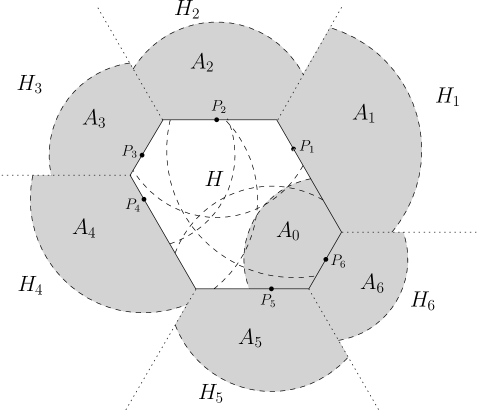
Figure 1: The circumscribed hexagon $H$ and associated regions.

Step 1: Defining the regions. We use the following hexagonal construction which was introduced by Balister, Bollobás, Sarkar and Walters in [2]. Let $H$ be the circumscribed hexagon of the points of $F$ obtained by taking the six tangents to the convex hull of $F$ at angles $0$ and $\pm 60^{\circ}$ to the horizontal,and let $H_{1},\ldots,H_{6}$ be the regions bounded by the exterior angle bisectors of $H$ as in Figure 1. Let $P_{1},\ldots,P_{6}$ be the points of $F$ on these tangents, and let $D_{1},\ldots,D_{6}$ denote the $k$-nearest neighbour disks of $P_{1},\ldots,P_{6}$. For $1\leq i\leq 6$ let $A_{i}=D_{i}\cap H_{i}$. Let $A_{0}$ be the set $D_{i}\cap H$ with the smallest area. We see that for each $1\leq i\leq 6$ the set $A_{i}$ contains no points of ${\mathcal{P}}$. Also $A_{0}$ contains $k+1$ points all of which must be in $F$ and thus in $A$. Writing $A^{\prime}$ for the set $A_{0}\cap A$, we see that $A^{\prime}$ contains at least $k+1$ points of ${\mathcal{P}}$.

We also wish to take account of points near to but not contained in $F$. Let $P\in F$ and $Q\in G\setminus F$ be vertices minimising the distance between $F$ and $G\setminus F$. Let $r_{0}=d(P,Q)$ and $r=r_{0}-\sqrt{2}s$. Since, we are assuming that every square of $A$ contains a point in $F$ we see that $A_{(r)}\setminus A$ contains no point of ${\mathcal{P}}$. Indeed, suppose there is a point of ${\mathcal{P}}$ in $A_{(r)}\setminus A$. Then this point is in $G\setminus F$ and is within $r_{0}$ of some point of $F$ which contradicts the definition of $r_{0}$.

Obviously the points $Q$ and $P$ are not joined so, in particular, the $k$ points nearest to $Q$ must all be nearer to $Q$ than $P$ is. Moreover, since $Q$ is the point closest to $F$, we see that these $k$ points must all be further away from $P$ than $Q$ is. Combining these we see that these $k$ points lie in in the set $B=D(Q,r_{0})\setminus D(P,r_{0})$.

Summarising all of the above, we see that $A^{\prime}$ and $B$ each contain at least $k$ points and $A_{(r)}\setminus A$ and $\bigcup_{i=1}^{6}A_{i}$ are both empty. The intersection $A^{\prime}\cap B$ contains no points (so we can think of them as disjoint) but $A_{(r)}$ and $\bigcup_{i=1}^{6}A_{i}$ will overlap significantly. Thus we will use Lemma 3 to form two separate bounds, one based on $A_{(r)}\setminus A$ being empty and one based on $\bigcup_{i=1}^{6}A_{i}$ being empty.

Step 2: Bounding the area of the regions. In this step we assume that the configuration is good.

First we bound $|\bigcup_{i=1}^{6}A_{i}|$. Since the configuration is good each disc $D_{i}$ has radius at most $c^{\prime}\sqrt{\log n}$ and each point $P_{i}$ is more than $2c^{\prime}\sqrt{\log n}$ from the boundary of $S_{n}$. In particular $D_{i}$ is contained in $S_{n}$ for each $i$. Moreover, since $|D_{i}\cap H_{i}|\geq|D_{i}\cap H|$ for each $1\leq i\leq 6$, we see that $|A_{i}|\geq|A_{0}|$. Since the $H_{i}$ and therefore the $A_{i}$ are disjoint, we have

$$|\bigcup_{i=1}^{6}A_{i}|\geq 6|A_{0}|\geq 6|A^{\prime}|.$$

The sets $B$ and $A_{(r)}$ both depend on $r$ so it is convenient to write $r$ in terms of $|A^{\prime}|$ by letting $x=r/(\sqrt{|A^{\prime}|/\pi})$.

Since $B=D(Q,r_{0})\setminus D(P,r_{0})$ a simple calculation shows that $|B|=\left(\frac{\pi}{3}+\frac{\sqrt{3}}{2}\right)r_{0}^{2}$. Since the configuration is good, $r_{0}>20000s$ so

$$r=r_{0}-\sqrt{2}s>r_{0}(1-10^{-4}).$$

Hence,

$$|B|=\left(\frac{\pi}{3}+\frac{\sqrt{3}}{2}\right)r_{0}^{2}\leq\left(\frac{\pi}{3}+\frac{\sqrt{3}}{2}\right)\frac{x^{2}|A^{\prime}|}{\pi(1-10^{-4})^{2}}<0.61x^{2}|A^{\prime}|.$$

Finally we bound $A_{(r)}$. Let $D$ and $D^{\prime}$ be balls of area $|A|$ and $|A^{\prime}|$ respectively. Since the configuration is good the the half-disc of radius $c^{\prime}\sqrt{\log n}$ about the right-most point of $F$ must contain a point of ${\mathcal{P}}$. In particular $r<r_{0}\leq c^{\prime}\sqrt{\log n}$, and so $A_{(r)}$ is contained in $S_{n}$. By the isoperimetric inequality in the plane

$$|A_{(r)}\setminus A|\geq|D_{(r)}\setminus D|,$$

and it easy to see that $|D_{(r)}\setminus D|\geq|D_{(r)}^{\prime}\setminus D^{\prime}|$. Since $D^{\prime}$ is a ball of radius $\sqrt{|A^{\prime}|/\pi}$, $D_{(r)}^{\prime}$ is a ball of radius $\sqrt{|A^{\prime}|/\pi}+r=(1+x)\sqrt{|A^{\prime}|/\pi}$, and we have

$$|D_{(r)}^{\prime}\setminus D^{\prime}|=((x+1)^{2}-1)|A^{\prime}|.$$

Step 3: Bounding the probability of such a configuration. We have seen that if there is such a component $F$ then there exist regions as defined in Step 1. These regions are determined by 14 points: the six points defining sides of the hexagonal hull, their six $k^{\rm th}$ nearest neighbour points and the points $P$ and $Q$; that is, if there is such a component $F$ then there are 14 points of ${\mathcal{P}}$ defining regions $A^{\prime}$, $B$, $A_{1},\ldots,A_{6}$ and $A_{(r)}$ with $\#A^{\prime}\geq k$, $\#B\geq k$, $\#(A^{\prime}\cap B)=0$, and both $\#\bigcup_{i=1}^{6}A_{i}=0$ and $\#(A_{(r)}\setminus A)=0$. Moreover, if the configuration is good all of these points must lie within $c^{\prime}\sqrt{\log n}$ of $A$.

Let $Z$ be the event that there are 14 points of ${\mathcal{P}}$ all within $c^{\prime}\sqrt{\log n}$ of $A$ defining regions with the above properties. We have

$$\mathbb{P}(\text{there exists }F \text{ and the configuration is good})$$

$$\leq\mathbb{P}(\text{Z and the configuration is good})$$

$$\leq\mathbb{P}(Z).$$

We bound the probability that $Z$ occurs (note we are not assuming that the configuration is good). Fix a particular collection of 14 points of ${\mathcal{P}}$ and let $Z^{\prime}$ be the event that these particular points witness $Z$. Note, since we are assuming these 14 points all lie with $c^{\prime}\sqrt{\log n}$ of $A$, the corresponding regions all lie entirely within $S_{n}$.

We apply Lemma 6 to the sets $A^{\prime}$, $B$ together with each of $\bigcup_{i=1}^{6}A_{i}$ and $A_{(r)}\setminus A$.

First we form the bound based on $\#\bigcup_{i=1}^{6}A_{i}=0$. We have $|A^{\prime}|\leq|\bigcup_{i=1}^{6}A_{i}|$ and, provided $x<3.13$, we have $|B|\leq 0.61x^{2}<6|A^{\prime}|\leq|\bigcup_{i=1}^{6}A_{i}|$ so Lemma 6 applies. Thus we see that

$$\mathbb{P}(Z^{\prime})\leq\left(\frac{4|A^{\prime}||B|}{(|A^{\prime}|+|(\bigcup_{i=1}^{6}A_{i})|+|B|)^{2}}\right)^{k}\leq\left(\frac{4\cdot 0.61x^{2}}{(7+0.61x^{2})^{2}}\right)^{k}.$$

Secondly we form a bound based on $\#(A_{(r)}\setminus A)=0$. This time $|B|\leq 0.61x^{2}|A^{\prime}|\leq((x+1)^{2}-1)|A^{\prime}|\leq|A_{(r)}\setminus A|$ and, provided that $x>\sqrt{2}-1$, we have $|A_{(r)}\setminus A|\geq|A^{\prime}|$ so the conditions of Lemma 6 are satisfied. Thus

$$\mathbb{P}(Z^{\prime})\leq\left(\frac{4|A^{\prime}||B|}{(|A^{\prime}|+|A_{(r)}\setminus A|+|B|)^{2}}\right)^{k}\leq\left(\frac{4\cdot 0.61x^{2}}{((x+1)^{2}+0.61x^{2})^{2}}\right)^{k}.$$

It is easy to check that the maximum of the minimum of these two bounds occurs when they are equal, i.e., when $x=\sqrt{7}-1$; at this point they are $\alpha^{-k}$ for some $\alpha>11.3$. Therefore $\mathbb{P}(Z^{\prime})\leq\alpha^{-k}$.

Since all 14 points must lie within $c^{\prime}\sqrt{\log n}$ of $A$ there are $O((\log n)^{14})$ ways of choosing them. Hence, the expected number of 14 point sets for which $Z^{\prime}$ occurs is is $O((\log n)^{14}\alpha^{-k})=O(11.3^{-k})$. Thus $\mathbb{P}(Z)=O(11.3^{-k})$ and the proof of the lemma is complete. ∎

Since the degree of vertices in $\widehat{G}$ is bounded and $16(c^{\prime}M)^{2}$ is a (large) constant, there are only a constant number of connected sets of $\widehat{G}$ of size at most $16(c^{\prime}M)^{2}$ which contain a fixed tile, and therefore $O(n)$ such sets in total. Since $k>0.4125\log n>\frac{1}{\log 11.3}\log n$ the expected number of small components in $G$ with the configuration good is $O(n(11.3)^{k})=o(1)$. Thus

$$\mathbb{P}(\text{$G$ is not} \text{ connected})$$

$$\leq\mathbb{P}(\text{there is a small component and ${\mathcal{P}}$ is good})+\mathbb{P}(\text{${\mathcal{P}}$ is bad})$$

$$=o(1)+O(n^{-\varepsilon})$$

$$=o(1),$$

so whp $G$ is connected.∎

4 Proof of Theorem 1

Much of this is the same as the proof of Theorem 2 so we shall concentrate on the differences. This time, by hypothesis we have $k>0.272\log n$ and again we may assume $k<0.6\log n$. We use exactly the same tesselation of $S_{n}$ with small squares of side length $s=\sqrt{\log n}/M$ where $c^{\prime}=\max\{c_{1}(0.25,1),c_{2}(0.25,1)\}$ and $M=20000c^{\prime}$ are given by Lemmas 3 and 5 as before. Again we form a graph $\widehat{G}$ on these tiles by joining two tiles whenever the distance between their centres is at most $2c^{\prime}\sqrt{\log n}$.

We need a slightly different definition of a bad pointset: the first four conditions are exactly as before but we replace the fifth condtion by

1. there exists a component of diameter at most $c^{\prime}\sqrt{\log n}$ containing a vertex within distance $3c^{\prime}\sqrt{\log n}$ of two sides of $S_{n}$.

Note that this condition, together with Condition 4 on the diameter of small components, implies that for any small component at most one side of $S_{n}$ can have points of this small component within distance $2c^{\prime}\sqrt{\log n}$ of it.

Since the tesselation is the same as in the proof of Theorem 2 we see that the probability that any of the original four conditions hold is $O(n^{-1})$ as before. Since $k>0.272\log n$ Lemma 4 implies that the probability of the new condition above is $O(n^{-\varepsilon})$ for some $0<\varepsilon<1$. Combining these we see that the probability of a bad configuration is $O(n^{-\varepsilon})$.

Suppose that ${\mathcal{P}}$ is a good configuration but not all points within $\log n$ of the boundary of $S_{n}$ are contained in the giant component. Then there exists a component $F$ with diameter at most $c^{\prime}\sqrt{\log n}$ containing a vertex within $\log n$ of the boundary of $S_{n}$. Let $A$ be the collection of tiles that contain a point of $F$. Since the configuration is good $A$ is a connected subset of $\widehat{G}$ and, as before, the bound on the diameter of $F$ implies that $A$ contains at most $16(c^{\prime}M)^{2}$ tiles. This time at most one side of $S_{n}$ has any tiles of $A$ within $c^{\prime}\sqrt{\log n}$ of it.

The following lemma, which is similar to Lemma 7 bounds the probability of such a small component.

Lemma 8.

Suppose $A$ is a connected subset of $\widehat{G}$ such that at most one side of $S_{n}$ has any tiles in $A$ within $c^{\prime}\sqrt{\log n}$ of it. The probability that the configuration is good and that $G$ has a small component contained entirely inside $A$ which meets every square of $A$ is at most $(6.3)^{-k}$.

Remark.

Obviously this lemma is only of interest for sets $A$ near the boundary, since otherwise Lemma 7 is stronger.

Proof.

The proof divides into the same three steps as Lemma 7.

Step 1: Defining the regions. As before suppose that $F$ is a component of $G$ meeting every tile in $A$. Let $E$ be the (almost surely unique) side of $S_{n}$ closest to $F$.

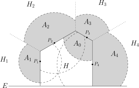
Figure 2: The circumscribing set $H$ and associated regions.

This time let $H$ be the region bounded by the four interior sides of the circumscribed hexagon of the points of $F$ obtained by taking four of the tangents to the convex hull of $F$ at angles $90^{\circ}$ and $\pm 30^{\circ}$ to $E$, together with $E$ as in Figure 2. Let $H_{1},\ldots,H_{4}$ be the regions bounded by the exterior angle bisectors of $H$ and $E$. Let $P_{1},\ldots,P_{4}$ be the points of $F$ on these tangents, and let $D_{1},\ldots,D_{4}$ denote the $k$-nearest neighbour disks of $P_{1},\ldots,P_{4}$. For $1\leq i\leq 4$ let $A_{i}=D_{i}\cap H_{i}$. Let $A_{0}$ be the set $D_{i}\cap H$ with the smallest area and write $A^{\prime}$ for the set $A_{0}\cap A$. Exactly as before we see that for $1\leq i\leq 4$ the set $A_{i}$ is empty, and that $A^{\prime}$ must contain at least $k+1$ points of ${\mathcal{P}}$.

As before let $P\in F$ and $Q\in G\setminus F$ be vertices minimising the distance between $F$ and $G\setminus F$, $r_{0}=d(P,Q)$ and $r=r_{0}-\sqrt{2}s$. Again, since $F$ meets every tile of $A$ we see that $A_{(r)}\setminus A$ must be empty. Also, as before, the set $B=(D(Q,r_{0})\setminus D(P,r_{0}))\cap S_{n}$ must contain at least $k$ points.

Step 2: Bounding the area of the regions. In this step we assume the configuration is good.

First we bound $|\bigcup_{i=1}^{4}A_{i}|$. Similarly to before we see that each disc $D_{i}$ has radius at most $c^{\prime}\sqrt{\log n}$ so meets no side of $S_{n}$ apart from possibly $E$. Thus, we have $|D_{i}\cap H_{i}|\geq|D_{i}\cap H|$ for each $1\leq i\leq 4$, so we see that $|A_{i}|\geq|A_{0}|$. As before the $H_{i}$ and therefore the $A_{i}$ are disjoint so

$$|\bigcup_{i=1}^{4}A_{i}|\geq 4|A_{0}|\geq 4|A^{\prime}|.$$

As before let $x=r/\sqrt{|A^{\prime}|/\pi}$ and exactly as in the proof of Lemma 7 we have $|B|<0.61x^{2}|A^{\prime}|$.

Finally we bound $A_{(r)}\setminus A$. Consider the point of $F$ furthest from $E$ and the half disc of radius $c^{\prime}\sqrt{\log n}$ about that point facing away from $E$. Since no point of $F$ is within $c^{\prime}\sqrt{\log n}$ of any side of $S_{n}$ apart from $E$, this half disc is entirely inside $S_{n}$, and so must contain a point of ${\mathcal{P}}$ (which is obviously not in $F$). Therefore, as before, $r<r_{0}\leq c^{\prime}\sqrt{\log n}$. Thus $A_{(r)}\cap S_{n}=A_{(r)}\cap E_{+}$ where $E_{+}$ denotes the halfplane bounded by $E$ that contains $S_{n}$.

This time let $D$ and $D^{\prime}$ be half discs of area $|A|$ and $|A^{\prime}|$ respectively centred on $E$. Then, by the isoperimetric inequality in the half plane $E_{+}$ (an easy consequence of the same inequality in the whole plane),

$$|(A_{(r)}\cap E_{+})\setminus A|\geq|(D_{(r)}\cap E_{+})\setminus D|\geq|(D_{(r)}^{\prime}\cap E_{+})\setminus D^{\prime}|.$$

Now $D^{\prime}$ is half a disc of radius $\sqrt{2}\sqrt{|A^{\prime}|/\pi}$ and $D_{(r)}^{\prime}\cap E_{+}$ is half a disc of radius $\sqrt{2}\sqrt{|A^{\prime}|/\pi}+r=(1+x/\sqrt{2})\sqrt{2|A^{\prime}|/\pi}$, so this time we we have

$$|(D_{(r)}^{\prime}\cap E_{+})\setminus D^{\prime}|=((1+x/\sqrt{2})^{2}-1)|A^{\prime}|.$$

Step 3: Bounding the probability of such a configuration. We have seen that if there is such a component $F$ then there exist regions as defined above. These regions are determined by 10 points: the four points defining sides of the hexagonal hull, their four $k^{\rm th}$ nearest neighbour points and the points $P$ and $Q$; that is, if there is such a component $F$ then there are 10 points of ${\mathcal{P}}$ defining regions $A^{\prime}$, $B$, $A_{1},\ldots,A_{4}$ and $A_{(r)}$ with $\#A^{\prime}\geq k$, $\#B\geq k$, $\#(A^{\prime}\cap B)=0$, and both $\#\bigcup_{i=1}^{4}A_{i}=0$ and $\#((A_{(r)}\cap S_{n})\setminus A)=0$. Again, if the configuration is good, all these points must lie within $c^{\prime}\sqrt{\log n}$ of $A$.

Similarly to before, let $Z$ be the event that there are 10 points of ${\mathcal{P}}$ all within $c^{\prime}\sqrt{\log n}$ of $A$ defining regions with the above properties. Again

$$\mathbb{P}(\text{there exists }F \text{ and the configuration is good})$$

$$\leq\mathbb{P}(\text{Z and the configuration is good})$$

$$\leq\mathbb{P}(Z)$$

so, as before, we bound $\mathbb{P}(Z)$.

Fix a particular collection of 10 points and let $Z^{\prime}$ be the event that these 10 points witness $Z$. Note, since we are assuming these 10 points all lie with $c^{\prime}\sqrt{\log n}$ of $A$, the regions $A^{\prime},A_{1},\ldots,A_{4}$ all lie entirely within $S_{n}$. By definition, $B$ and $(A_{(r)}\cap S_{n})\setminus A$ also lie in $S_{n}$.

Again we apply Lemma 6 to the sets $A^{\prime}$, $B$ together with each of $\bigcup_{i=1}^{4}A_{i}$ and $(A_{(r)}\cap S_{n})\setminus A$. This time, however, neither bound will be valid for large $x$ so we form a third bound based just on the two sets $A^{\prime}$ and $(A_{(r)}\cap S_{n})\setminus A$.

As before we base the first bound on $\#\bigcup_{i=1}^{4}A_{i}=0$. We have $|A^{\prime}|\leq|\bigcup_{i=1}^{4}A_{i}|$ and, provided $x<2.56$, we have $|B|\leq 0.61x^{2}|A^{\prime}|<4|A^{\prime}|\leq|\bigcup_{i=1}^{4}A_{i}|$ so Lemma 6 implies

$$\mathbb{P}(Z^{\prime})\leq\left(\frac{4|A^{\prime}||B|}{(|A^{\prime}|+|(\bigcup_{i=1}^{4}A_{i})|+|B|)^{2}}\right)^{k}\leq\left(\frac{4\cdot 0.61x^{2}}{(5+0.61x^{2})^{2}}\right)^{k}.$$

The second bound based on $\#((A_{(r)}\cap S_{n})\setminus A)=0$ is also very similar to before. However, this time the middle inequality in

$$|B|\leq 0.61x^{2}|A^{\prime}|\leq((1+x/\sqrt{2})^{2}-1)|A^{\prime}|\leq|(A_{(r)}\cap S_{n})\setminus A|$$

is not valid for all $x$, but it is valid for all $x<12$. Also provided that $x>2-\sqrt{2}$, we have $|(A_{(r)}\cap S_{n})\setminus A|\geq|A^{\prime}|$ so for $2-\sqrt{2}<x<12$ the conditions of Lemma 6 are satisfied. Thus

$$\mathbb{P}(Z^{\prime})\leq\left(\frac{4|A^{\prime}||B|}{(|A^{\prime}|+|(A_{(r)}\cap S_{n})\setminus A|+|B|)^{2}}\right)^{k}\leq\left(\frac{4\cdot 0.61x^{2}}{((1+x/\sqrt{2})^{2}+0.61x^{2})^{2}}\right)^{k}.$$

Since neither bound applies for large $x$ we form a third bound based on the two sets $A^{\prime}$ and $(A_{(r)}\cap S_{n})\setminus A$. We know $A^{\prime}$ contains at least $k$ points and $(A_{(r)}\cap S_{n})\setminus A$ is empty. This has probability at most

$$\mathbb{P}(Z^{\prime})\leq\left(\frac{|A^{\prime}|}{|A^{\prime}|+|(A_{(r)}\cap S_{n})\setminus A|}\right)^{k}\leq\frac{1}{(1+x/\sqrt{2})^{2k}}$$

which is less than $80^{-k}$ for all $x\geq 12$.

As before the maximum of the minimum of the first two bounds occurs when they are equal at $x=\sqrt{2}(\sqrt{5}-1)$; at this point they are $\alpha^{-k}$ for some $\alpha>6.3$. Moreover the third bound is tiny in comparison. Thus, in all cases, $\mathbb{P}(Z^{\prime})\leq\alpha^{-k}$ for some $\alpha>6.3$.

Since all 10 points must lie within $c^{\prime}\sqrt{\log n}$ of $A$ there are $O((\log n)^{10})$ ways of choosing them. Hence, similarly to before, the expected number of 10 point sets for which $Z^{\prime}$ occurs is is $O((\log n)^{10}\alpha^{-k})=O(6.3^{-k})$. Hence $\mathbb{P}(Z)=O(6.3^{-k})$ and the proof of the lemma is complete. ∎

The remainder of the proof is very similar to before. There are only a constant number of connected sets of $\widehat{G}$ of size at most $16(c^{\prime}M)^{2}$ which contain a fixed tile, and therefore $O(\sqrt{n\log n})$ such sets which contain a tile within distance $\log n$ of the boundary of $S_{n}$. Since $k>0.272\log n>\frac{1+\varepsilon^{\prime}}{\log 6.3}\log(\sqrt{n})$ for some $\varepsilon^{\prime}>0$ the expected number of small components of $G$ that contain a vertex within distance $\log n$ of the boundary of $S_{n}$ when the configuration is good is $O(\sqrt{n\log n}(6.3)^{-k})=o(n^{-\varepsilon^{\prime}/2})$. Let $\varepsilon=\min(\varepsilon^{\prime}/2,1)$ and $p$ be the the probability that there exists a point ${\mathcal{P}}$ within $\log n$ of the boundary of $S_{n}$ that is not in the giant component. Then

$$p \leq\mathbb{P}(\text{there is a small boundary component and ${\mathcal{P}}$ is good})+\mathbb{P}(\text{${\mathcal{P}}$ is bad})$$

$$=o(n^{-\varepsilon})+O(n^{-\varepsilon})$$

$$=O(n^{-\varepsilon})$$

as claimed.∎

Open Questions

In this paper we have proved two results about the behaviour of the small components in the graph $G_{n,k}$. However, several question about their properties remain open. We are interested in the behaviour near the connectivity threshold so, in particular, we assume in the following questions that $k$ is at least $0.3\log n$.

Question 1.

Must the small components of $G_{n,k}$ be isolated? More precisely, is it the case that, whp, there do not exist two small components within distance of $O(\sqrt{\log n})$ of each other.

Since the first draft of this paper Falgas-Ravry [4] has answered this question in the affirmative provided that the probability that $G$ is connected is not too small: more precisely he proves it whenever $\mathbb{P}(G$ is connected$)=\Omega(n^{\gamma})$ (where $\gamma$ is an absolute constant).

Question 2.

How many vertices do small components contain?

It is immediate from Lemma 6 of [2] (quoted as Lemma 3 of this paper) that all small components contain $O(k)$ vertices. If the lower bound construction of Balister, Bollobás, Sarkar and Walters in [2] is extremal then, as the authors remark there, all small components would contain $k+O(1)$ vertices.

Question 3.

Are all the small components convex in the sense that all points of ${\mathcal{P}}$ within the convex hull of a small component are actually part of the small component?

References

- [1] N. Alon and J. H. Spencer. The probabilistic method. Wiley-Interscience Series in Discrete Mathematics and Optimization. John Wiley & Sons Inc., Hoboken, NJ, third edition, 2008.
- [2] P. Balister, B. Bollobás, A. Sarkar, and M. Walters. Connectivity of random -nearest-neighbour graphs. Adv. in Appl. Probab., 37(1):1–24, 2005.
- [3] P. Balister, B. Bollobás, A. Sarkar, and M. Walters. A critical constant for the -nearest-neighbour model. Adv. in Appl. Probab., 41(1):1–12, 2009.
- [4] V. Falgas-Ravry. On the distribution of small components in the -nearest neighbours random geometric graph model. Preprint.
- [5] F. Xue and P. R. Kumar. The number of neighbors needed for connectivity of wireless networks. Wireless Networks, 10:169–181, 2004.