The Satellite Luminosity Functions of Galaxies in SDSS

Abstract

We study the luminosity function of satellite galaxies around isolated primaries using the Sloan Digital Sky Survey (SDSS) spectroscopic and photometric galaxy samples. We select isolated primaries from the spectroscopic sample and search for potential satellites in the much deeper photometric sample. For primaries of similar luminosity to the Milky Way and M31, we are able to stack as many as $\sim\negthinspace 20,000$ galaxy systems to obtain robust statistical results. We derive the satellite luminosity function extending almost 8 magnitudes fainter than the primary galaxy. We also determine how the satellite luminosity function varies with the luminosity, colour and concentration of the primary. We find that, in the mean, isolated primaries of comparable luminosity to the Milky Way and M31 contain about a factor of two fewer satellites brighter than $M_{V}=-14$ than the average of the Milky Way and M31.

1 Introduction

The $\rm{\Lambda CDM}$ model predicts that structure forms in a hierarchical manner. Large spiral galaxies like the Milky Way (MW) and M31 form within extended dark matter halos from the merging and accretion of smaller subhalos. Smaller structures falling into bigger haloes can survive there as substructures and host observed satellite galaxies. A strong prediction of the theory, borne out by high resolution N-body simulations, is that a very large number of such dark matter substructures should survive in galactic halos (Klypin et al., 1999; Moore et al., 1999; Diemand, Kuhlen & Madau, 2007; Springel et al., 2008). Empirical tests of this prediction have so far been restricted to a single system, the Local Group, the only one for which an estimate of the satellite luminosity function (LF) is readily available. Indeed, Klypin et al. (1999) and Moore et al. (1999) noted that the observed number of satellites around the MW and M31 is much smaller than the number of predicted substructures, giving rise to the so-called “missing satellites problem” of the $\rm{\Lambda CDM}$ model.

In the past decade or so, fainter satellites around the MW and M31 have been discovered in the SDSS (e.g. Belokurov et al., 2008, 2010; Grebel, 2000; Irwin et al., 2007; Liu et al., 2008; Martin et al., 2006; Martin et al., 2008; Simon & Geha, 2007; van den Bergh, 2000; Watkins et al., 2009; Zucker et al., 2004, 2006, 2007), but the number is still orders of magnitude smaller than the predicted number of surviving cold dark matter subhalos. A number of solutions to this problem have been proposed. Some invoke a different kind of dark matter, warm dark matter, in which case the number of surviving substructures is dramatically reduced by a cutoff in the primordial power spectrum (Moore et al., 2000; Spergel & Steinhardt, 2000; Yoshida et al., 2000; Bode, Ostriker, & Turok, 2001; Craig & Davis, 2001; Lovell et al., 2011). Others retain cold dark matter and appeal to galaxy formation processes, such as photoionization and supernova feedback, to inhibit star formation in small subhalos thus rendering most of them invisible. This idea, first mentioned nearly 20 years ago by Kauffmann et al. (1993), was worked out in detail a decade later using analytical arguments and semi-analytical models (Bullock, Kravtsov & Weinberg, 2000; Benson et al., 2002; Somerville, 2002).

The discovery of new Local Group satellites in the SDSS has stimulated further observational and, particularly, theoretical work. Koposov et al. (2008) and Tollerud et al. (2008) extended the estimate of the satellite LF of the MW and M31 to faint magnitudes, accounting for the survey magnitude limit and modelling the radial density profile of the satellite distribution. This extension to faint magnitudes agrees remarkably well with the $\rm{\Lambda CDM}$ model predictions of Benson et al. (2002), a result that has been confirmed in recent work using related semi-analytic modelling techniques (Koposov et al., 2009; Muñoz et al., 2009; Busha et al., 2010; Cooper et al., 2010; Macciò et al., 2010; Li, De Lucia, & Helmi, 2010; Font et al., 2011). Full N-body/gasdynamic simulations have also been carried out to investigate the physics of satellite galaxies (Libeskind et al. 2007; Okamoto & Frenk 2009; Okamoto et al. 2010; Wadepuhl & Springel 2010) although currently these simulations only resolve the brightest examples. In spite of this broad agreement, interesting discrepancies exist. For example, the original model of Benson et al. (2002), as well as the more recent model by Guo et al. (2010), rarely produce satellites as bright as the LMC and SMC (Boylan-Kolchin et al., 2010).

The large body of work on satellite galaxies reflects the importance of these objects as a critical test of the $\rm{\Lambda CDM}$ model on small scales. Yet, all conclusions to date regarding the validity or otherwise of the model rely on comparison with data for a few dozen satellites around just two galaxies, the MW and M31. There is no guarantee that these are typical and indeed there is good evidence that the satellites of the two galaxies have different structural properties (McConnachie & Irwin, 2006; Collins et al., 2010). Clearly, robust and reliable tests of cosmological and galaxy formation models require comparison with statistically representative samples of galaxies and their satellites.

Analyzing the satellite sytems of external galaxies is challenging because typically only one or two satellites are detected per primary galaxy (Holmberg, 1969; Lorrimer et al., 1994; Zaritsky et al., 1993, 1997b). In addition, the real space position of the satellite with respect to its primary is uncertain. To circumvent the first problem, these authors developed the method of stacking the primaries and their satellites in order to obtain a fair and complete sample which can yield statistically robust results for certain classes of primary galaxies. These early studies were limited by the relatively small samples available at the time. With the advent of large galaxy redshift surveys such as the 2dF Galaxy Redshift Survey (2dFGRS; Colless et al., 2001) and the Sloan Digital Sky Survey (SDSS; York et al., 2000), it is now possible to construct external galaxy samples covering a much larger volume. Studies with significantly improved statistics have been carried out using these new surveys (e.g. Sales & Lambas, 2004; Yang et al., 2006; Agustsson & Brainerd, 2010),

In this work, we are interested in the satellite luminosity function of specific types of isolated primary galaxies and, for this, the new spectroscopic surveys are still not deep enough. For example, even within the largest galaxy redshift catalogue from SDSS DR7 (Abazajian et al., 2009), where there are about $\sim\negthinspace 660\,000$ galaxies with $m_{r}^{\rm{lim}}<17.77$, only a relatively small number of isolated low redshift galaxy systems have enough detected satellites for our purposes (e.g. Hwang & Park, 2010). On the other hand, the photometric catalogue from SDSS DR7 contains $\sim\negthinspace 96\,000\,000$ galaxies with magnitudes in the $u,g,r,i,z$ bands (roughly $m_{r}^{\rm{lim}}\la 22$) and photometric redshifts. In this study, we used both the spectroscopic and photometric SDSS DR7 catalogues. To ensure completeness, we restrict the photometric sample in our main analysis to galaxies brighter than $m_{r}=20.5$ (see Section 4). The resulting catalogues enable us to analyze a sufficiently large statistical sample of galaxy systems. We construct our sample using methods similar to those developed by Lorrimer et al. (1994) but modified slightly to include photometric redshifts.

As this project was nearing completion, Liu et al. (2010) published an investigation using similar methods to quantify the frequency with which satellites as bright as the LMC and SMC occur around primaries similar to the MW. Shortly afterwards, Lares, Lambas, & Dominguez (2010) also published a similar study, focused on primaries brighter than $M_{r}<-20.5$, investigating how the satellite LF and projected density profile depend on the primary luminosity and colour. Our work complements these studies by including a wider range of primary luminosities and exploring how the satellite LF depends on the properties of the primary. Also, we adopt stricter isolation criteria than those of Lares, Lambas, & Dominguez (2010). We compare our results with those of these studies in the discussion in Section 5.

The remainder of this paper is organised as follows. In Section 2, we describe the selection of primary galaxies and their satellites; in Section 3, we develop the method of estimating the satellite LF; in Section 4, we present our estimate of the satellite LF for different types of primary galaxy. We conclude, in Section 5, with a summary and discussion of our results.

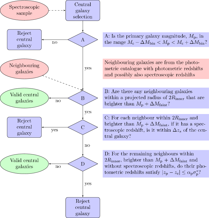
Figure 1: A flow chart detailing the selection criteria for isolated primary galaxies.

2 Data and Sample Selection

We build two different catalogues for our study: a smaller one of galaxies with spectroscopic redshifts from which we select the primary galaxies (hereafter the spectroscopic catalogue) and a larger one of galaxies with photometric redshifts and magnitudes from which we select the neighbouring galaxies (hereafter the photometric catalogue). The spectroscopic catalogue is constructed from the SDSS DR7 spectroscopic subsample (north galactic cap) including all objects with high quality redshifts (zconf $>0.7$ and specClass $=2$) and a Petrosian magnitude $r\leq 17.77$. The photometric galaxy catalogue is from the SDSS DR7 photometric subsample (north galactic cap) and includes only objects that have photometric redshifts, none of the flags BRIGHT, SATURATED, or SATUR_CENTER set and model magnitudes $r\leq 22.0$. We select only objects with corresponding entries in the SDSS database PhotoZ table, which naturally selects galaxies and excludes stars. As galaxies with $r\leq 17.77$ are included in both SDSS catalogues, a small fraction of the photometric catalogue galaxies also have spectroscopic redshifts. We use de-reddened model $ugriz$ magnitudes and k-correct all galaxies to $z=0$ with the IDL code of Blanton & Roweis (2007). In addition, we also include $V$-band magnitudes estimated from $g$ and $r$-band magnitudes assuming $V=g-0.55(g-r)-0.03$ (Smith et al., 2002). This allows us directly to compare our results with observations of the MW.

For our statistical analysis, the sample of primary galaxies should be not only homogeneous but also isolated. To this end, we adopt a series of selection criteria summarised in the flow chart shown in Fig. 1. First, from the spectroscopic sample, we select primary galaxy candidates of absolute magnitude, $M_{\rm p}$, in the range $M_{\rm{C}}-\Delta M_{\rm{bin}}<M_{\rm p}\leq M_{\rm{C}}+\Delta M_{\rm{bin}}$. We then reject from this list those candidates that have, or could have, bright neighbours whose own satellite system could overlap with that of the candidate. We achieve this by rejecting candidates that have a neighbouring galaxy within a projected distance of $2R_{\rm{inner}}$ that is brighter than $M_{\rm p}+\Delta M_{\rm faint}$, unless that neighbouring galaxy is at a substantially different redshift. For neighbours with spectroscopic redshifts, $z_{\rm s}$, the required redshift separation is $|z_{\rm p}-z_{\rm s}|>\Delta z_{s}$, while for those with only photometric redshifts, $z_{\rm phot}$, we require $|z_{\rm p}-z_{\rm phot}|>\alpha_{\rm p}\sigma^{*}_{p}$. Here $\sigma_{\rm p}^{*}$ is the photometric redshift error that we adopt (see Section 3) and $\alpha_{\rm p}$ is a tolerance, which we will vary. The isolation criteria guarantee that there are no luminous neighbouring galaxies that are projected within $2R_{\rm{inner}}$ of the primary, unless these luminous neighbours are sufficiently far away from the primary and appear here due to a chance projection. Using the photometric redshift information to identify and remove true background and foreground galaxies significantly increases the number of primary galaxies retained in our sample and reduces the background contamination.

Table 1: Properties of the primary galaxy samples for the following default choices of values for the sample selection parameters, $\{M_{\rm{c}},R_{\rm{inner}},R_{\rm{outer}},\Delta M_{\rm{bin}},\Delta M_{\rm{faint}},\Delta z_{\rm{s}},\alpha_{\rm{p}}\}=\{M_{\rm{c}},0.3~{}\rm{Mpc},0.6~{}\rm{Mpc},0.5,0.5,0.002,2.5\}$. Quantities listed for each bin of $V$-band absolute magnitude $M_{\rm{c}}$ are: the number of primary galaxy candidates (galaxies within the absolute magnitude bin), the number of primary galaxies that pass all the isolation criteria, their median redshift and redshift range.

$M_{\rm{c}}$	primary	primaries	median	redshift
	candidates		redshift	range
-19.0	35893	88	0.043	$0.021<z<0.066$
-20.0	104907	2661	0.105	$0.020<z<0.068$
-21.0	202351	21346	0.098	$0.016<z<0.164$
-22.0	94287	51733	0.142	$0.022<z<0.391$
-23.0	51686	26982	0.203	$0.031<z<0.522$

After having filtered by these criteria, the remaining isolated galaxies comprise the primary galaxy catalogue. We briefly summarise the properties of this catalogue. The number of primary galaxies not only depends on their absolute magnitude, but also on the isolation parameters. The stricter the isolation criteria we take, the fewer primary galaxies we have. In the $V$-band, with a parameter set $\{M_{\rm{c}},R_{\rm{inner}},R_{\rm{outer}},\Delta M_{\rm{bin}},\Delta M_{\rm{faint}},\Delta z_{\rm{s}},\alpha_{\rm{p}}\}=\{-21.0,0.3~{}\rm{Mpc},0.6~{}\rm{Mpc},0.5,0.5,0.002,2.5\}$, the number of candidates is 202 351, which, after applying the isolation criteria, is reduced to 21 346 or about 10% of the galaxies in this magnitude bin. The primary galaxy redshifts lie in the range $0.01<z<0.16$, with a median redshift $0.098$. For different primary magnitudes, $M_{\rm{c}}$, the number of primary galaxies and their median redshifts are shown in Table 1. For each magnitude bin, the number of primary candidates is determined by the interplay between the accessible volume given the survey limit and the density of galaxies. The actual number of primaries is further affected by the isolation criteria which, for example, tend to reject nearby galaxies for which $2R_{\rm inner}$ subtends a large angle.

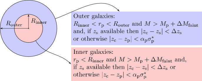
Figure 2: Schematic showing the selection of potential satellite galaxies within $R_{\rm{inner}}$ and of a reference sample within an annulus defined by $R_{\rm{inner}}<r<R_{\rm outer}$, used to subtract the residual contaminating background. For both samples we apply the stated redshift cuts to reduce background contamination. We also apply the stated absolute magnitude cut to both samples (assuming the neighbouring galaxies are at the same redshift as the primary) though this cut is redundant unless $R_{\rm{outer}}>2R_{\rm{inner}}$ as otherwise the existence of such bright neighbouring galaxies would automatically lead to the exclusion of the primary galaxy.

The schematic in Fig. 2 indicates our selection procedure for potential satellites or “inner galaxies”, and the corresponding selection of the “outer galaxies” used to define the background. We assume the satellites of the primary galaxy fall within a projected radius, $R_{\rm{inner}}$ (the red circle in Fig. 2). To reduce the background contamination, we apply the same cuts in redshift (spectroscopic and photometric) as were applied when selecting the primary galaxies, but as most of the galaxies within $R_{\rm{inner}}$ only have photometric redshifts with quite large measurement errors, we still cannot distinguish true satellites from projected background galaxies. However, the existence of satellites will make the number density of galaxies within $R_{\rm{inner}}$ slightly larger than that in the outer blue reference annulus in Fig. 2 ($R_{\rm{inner}}<r<R_{\rm{outer}}$). By counting the difference between the number density of galaxies within $R_{\rm{inner}}$ and in the reference annulus, we can estimate the number of true satellites.

An example of the objects we detect around a typical primary galaxy is shown in Fig. 3. This image, produced by the SDSS finding chart tool, illustrates the quality of the data and shows that candidate satellites are spatially well separated from the light distribution of the primary galaxy. The white circle (slightly stretched in this Aitoff projection) indicates $r=R_{\rm{inner}}$. Within this region we have marked all the galaxies in our catalogue with red circles and the subset brighter than $m_{r}=20.5$, used in our main analysis, with yellow boxes. The remaining visible objects within $R_{\rm{inner}}$ are not in our catalogue. Manual inspection with the DR7 Navigate tool reveals them to be classified as stars.

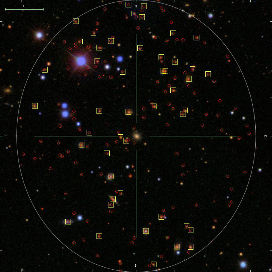
Figure 3: An example SDSS DR7 image centred on a primary galaxy of magnitude $m_{r}=16.10$ at redshift $z=0.074$. The white ellipse marks $r=R_{\rm{inner}}=300$ kpc. All catalogued galaxies projected within $R_{\rm{inner}}$ of the primary are marked with red circles. Those brighter than our fiducial $m_{r}=20.5$ magnitude limit are marked with yellow boxes. The remaining unmarked images within $R_{\rm{inner}}$ are presumed to be classified as stars, which we have verified in this case using the manual SDSS DR7 Navigate Tool.

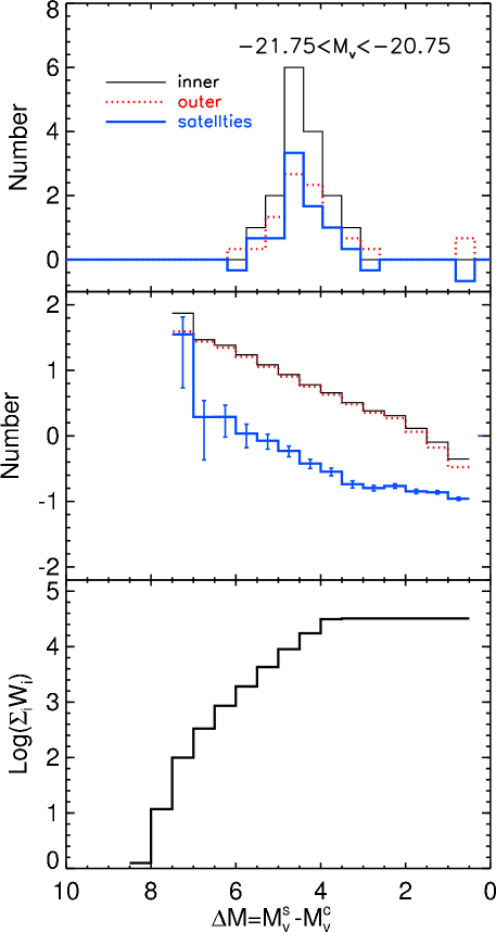
Figure 4: Estimation of the satellite luminosity function. The top panel shows the $V$-band LF for a single primary galaxy. The middle panel shows the mean satellite LF of all primary galaxies. The black (thin) and red (dotted) lines give the counts of inner and outer galaxies respectively and the blue (thick) lines the estimate of the satellite LF. The number of primary galaxies contributing to the mean satellite LF in each bin is shown in the bottom panel. Here the selection parameters, $\{R_{\rm{inner}},R_{\rm{outer}},\Delta M_{\rm{bin}},\Delta M_{\rm{faint}},\Delta z_{\rm{s}},\alpha_{\rm{p}}\}$, are set to the default values $\{-21.25,0.3~{}\rm{Mpc},0.6~{}\rm{Mpc},0.5,0.5,0.002,2.5\}$

3 Estimating the Satellite Luminosity Function

Once the primary galaxies are defined, their potential satellites are found from the photometric galaxy catalogue as depicted in Fig. 2. For the $i$th primary galaxy, the number of inner galaxies, $N^{\rm{inner}}_{i}(M)$, is found by counting all neighbouring galaxies within the inner area that satisfy the following conditions: at least $\Delta M_{\rm{faint}}$ fainter than the primary; if they have a spectroscopic redshift, $z_{\rm{s}}$, then it should satisfy $|z_{\rm{c}}-z_{\rm{s}}|<\Delta z_{\rm{s}}$; or if they only have a photometric redshift $z_{\rm{p}}$, then it should satisfy $|z_{\rm{c}}-z_{\rm{p}}|<\alpha_{\rm{p}}\sigma_{\rm{p}}^{*}$, where $\sigma_{\rm{p}}^{*}$ is the error in the photometric redshift as defined below. The number of outer galaxies, $N^{\rm{outer}}_{i}(M)$, is determined by applying the same conditions to galaxies in the outer area. As most satellites of the primary should be projected within $R_{\rm{inner}}$ of the primary, the number density of inner galaxies should typically exceed that of the outer galaxies. The excess can be taken as the projected satellite LF of the $i$th primary galaxy, and estimated by

$$N^{\rm{sat}}_{i}(M)=N^{\rm{inner}}_{i}(M)-\frac{A^{\rm{inner}}_{i}}{A^{\rm{outer}}_{i}}\,N^{\rm{outer}}_{i}(M),$$ (1)

where $A^{\rm{inner}}_{i}$ and $A^{\rm{outer}}_{i}$ are the areas of the inner and outer regions respectively (excluding sub-regions not within the sky coverage of the SDSS DR7, which we have identified using the mask described in Norberg et al. (2011)) .

Because of the survey apparent magnitude limit, we are able to probe less of the faint end of the satellite LF for primaries at higher redshift. To account for this and construct an unbiased estimate of the satellite LF averaged over all primary galaxies, we count the effective number of primaries contributing to each bin of the LF using the weighting function

$$W_{ij}(M_{j})=\left\{\begin{array}[]{ll}1&M_{j}<M_{i}^{\rm{lim}}+\Delta M_{j}\\ \frac{(M_{i}^{\rm{lim}}-\Delta M_{j}-M_{j})}{2\Delta M_{j}}&M_{i}^{\rm{lim}}-\Delta M_{j}\leq M_{j}\leq\\ &\qquad\qquad M_{i}^{\rm{lim}}+\Delta M_{j}\\ 0&M_{j}>M_{i}^{\rm{lim}}-\Delta M_{j}\end{array}\right.,$$ (2)

where $M_{j}$ is the central value of each magnitude bin, $\Delta M_{j}$ is the half width of the bin, $M_{i}^{\rm{lim}}=m^{\rm{lim}}-5\log_{10}(D^{L}_{i})-K(z_{i})$, $D^{L}_{i}$ is the luminosity distance of the i$th$ galaxy and $m^{\rm{lim}}$ is the SDSS galaxy spectroscopic sample magnitude limit. For a given primary, the weighting function is unity for all magnitude bins in which satellites anywhere in the bin are bright enough to be included in the survey. It is zero if all satellites within the bin are too faint to be included in the survey and ramps between zero and one when only galaxies in a fraction of the bin width are accessible to the survey. We then define the effective number of primary galaxies, $N^{\rm{prim}}_{j}$, contributing to the $j$th bin of the LF as $N^{\rm{prim}}_{j}=\sum_{i}W_{ij}(M_{j})$. With this definition, our unbiased estimator of the average satellite LF is given by

$${\widetilde{N}^{\rm{sat}}(M_{j})}=\frac{\sum_{i}N^{\rm{sat}}_{i}(M_{j})}{N^{\rm prim}_{j}}.$$ (3)

In practice, in our study we divide the satellite luminosities, $M_{j}$, into $20$ bins ($j=1,2,\cdots,20$). Furthermore, because each primary galaxy in the same bin has a slightly different magnitude relative to $M_{\rm{c}}$, we choose to show our results in terms of the difference in the magnitude of the satellite and primary galaxy, $\Delta M=M_{\rm{s}}-M_{\rm{p}}$, which aligns the satellite LFs in the same bin.

The process of estimating the satellite LF for primaries in one bin of $V$-band absolute magnitude is illustrated in Fig. 4. The thin black histogram in the top panel shows the number of inner galaxies binned by $V$-band magnitude difference for one of the primaries. The dotted red histogram shows the corresponding number of outer galaxies scaled by the ratio of areas ${A^{\rm{inner}}_{i}}/{A^{\rm{outer}}_{i}}$. Their difference, which is an estimate of the satellite LF in that system, is shown by the thick blue histogram. The thin black and dotted red histograms in the middle panel show the number of inner and (scaled) outer galaxies per primary where the number of primaries, $N^{\rm prim}_{j}=\sum_{i}W_{ij}(M_{j})$, contributing at each $\Delta M$ is shown in the lower panel. The heavy blue histogram in the middle panel of Fig. 4 shows the estimated mean satellite LF for all primaries in the magnitude range $-21.75<M_{\rm V}<-20.75$. The error bars on this mean satellite LF are estimated by bootstrap resampling of the set of primaries. At the faint end of the LF the error bars become quite large because of the small number of nearby primaries that are able to contribute. If the faintest bin only contains one primary then we show a Poisson, rather than the bootstrap error.

For a specific $M_{\rm{c}}$, the selection of primaries and counts of inner and outer galaxies are determined by the parameter set $\{R_{\rm{inner}},R_{\rm{outer}},\Delta M_{\rm{bin}},\Delta M_{\rm{faint}},\Delta z_{\rm{s}},\alpha_{\rm{p}}\}$. It is important to choose appropriate values for these parameters. Here we discuss the physical motivation for our choice of parameter values and check that the resulting satellite luminosity function is robust to reasonable variations in these parameters. The various panels in Fig. 5 show the results of varying these parameters away from our default choice of $\{M_{\rm{c}},R_{\rm{inner}},R_{\rm{outer}},\Delta M_{\rm{bin}},\Delta M_{\rm{faint}},\Delta z_{\rm{s}},\alpha_{\rm{p}}\}=\{M_{\rm{c}},0.3~{}\rm{Mpc},0.6~{}\rm{Mpc},0.5,0.5,0.002,2.5\}$.

The area within which we search for the satellite signal is determined by the parameter $R_{\rm{inner}}$. For too small a value of $R_{\rm{inner}}$, we would lose genuine satellites. Once $R_{\rm{inner}}$ is sufficiently large to enclose all the true satellites the resulting background-subtracted satellite LF should be independent of $R_{\rm{inner}}$. However, the statistical error in the estimate will increase due to increased background contamination. The value of $0.3~{}\rm{Mpc}$ is roughly the virial radius of the Milky Way, and so this seems a reasonable value to take for the $R_{\rm{inner}}$ of Milky Way-like primary galaxies. One could argue for scaling $R_{\rm{inner}}$ with the magnitude or type of the primary galaxy, but, for simplicity, we set $R_{\rm{inner}}=0.3~{}\rm{Mpc}$ in this study except in our parameter tests. In Fig. 5a, we show that the effect of varying $R_{\rm{inner}}$ between $0.25$ and $0.35$ Mpc does not change the satellite LF significantly. A possible concern is that the SDSS data reduction pipeline occasionally misclassifies fragments of the spiral arms of bright galaxies as separate galaxies. We have checked that these contaminating objects do not make a significant contribution to our estimate of the satellite luminosity by excluding all galaxies within $1.5$ times the Petrosian $R_{90}$ radius of the primary galaxies. Comparison of the resulting satellite luminosity functions shows that they make no significant difference.

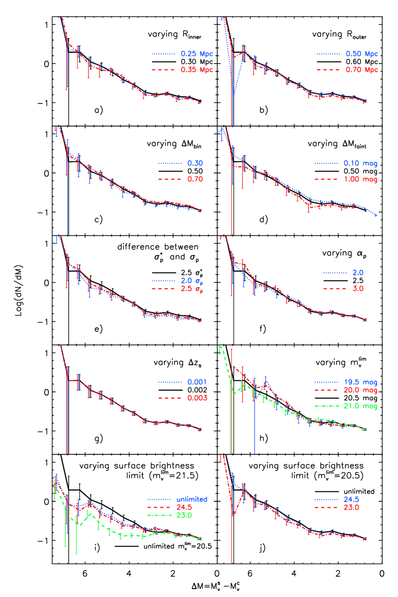
Figure 5: The effect on the estimated satellite LF of varying the parameters $\{R_{\rm{inner}},R_{\rm{outer}},\Delta M_{\rm{bin}},\Delta M_{\rm{faint}},\Delta z_{\rm{s}},\alpha_{\rm{p}}\}$ from their default values, $\{-21.25,0.3~{}\rm{Mpc},0.6~{}\rm{Mpc},0.5,0.5,0.002,2.5\}$, as indicated in the legends. In addition, panel e shows the effect of changing the assumed photometric redshift error from the original $\sigma_{\rm p}$ to our adopted $\sigma_{\rm p}^{*}=\max(\sigma_{\rm p},0.05)$ . Panels h,i and j show the effect of varying the apparent magnitude limit of the photometric catalogue and imposing an additional cut on surface brightness (see text for details). In this and in Figs. 6, 7 and 9, the error bars for different datasets have been slightly shifted for clarity.

The next parameter, $R_{\rm{outer}}$, determines the outer reference annulus from which we estimate “background” counts. An appropriate value for $R_{\rm{outer}}$ will guarantee a suitably local estimate of the background. A local estimate of the background is preferable (see Chen et al., 2006) as galaxies are clustered and, in our case, the mean environment of a primary galaxy is also biased by the isolation criteria that we apply. Fig. 5b shows that, provided the outer area is sufficiently large to allow an accurate estimate of the background, the resulting satellite LF is robust to changes in $R_{\rm{outer}}$. We also tested the effect of estimating the background using a larger annulus that was disjoint from the inner region (from $0.5$ Mpc to $0.7$ Mpc ) and again found no significant difference.

Besides the physically motivated parameters, we also test the parameters of the estimation method. For a specific central magnitude, $M_{\rm{c}}$, the bin half width, $\Delta M_{\rm{bin}}$, is a compromise between having a large enough sample of primary galaxies and not distorting the LF due to averaging over primaries of differing luminosities. Fig. 5c shows results for a few different $\Delta M_{\rm{bin}}$ values and indicates that, for our choice of binning, the satellite LF by the magnitude difference, $\Delta M=M_{\rm s}-M_{\rm p}$, any biases are very small.

The next panel, Fig. 5d, shows the effect of varying the parameter $\Delta M_{\rm{faint}}$, which is important in selecting isolated primaries. The larger $\Delta M_{\rm{faint}}$, the smaller the number of primary galaxies that survive the isolation filter. Hence, the value of $\Delta M_{\rm{faint}}$ is a compromise between avoiding the introduction of primary galaxies within groups and gathering sufficient primary galaxies. We adopt $\Delta M_{\rm{faint}}=0.5$, but Fig. 5d shows that, apart from the truncation of the satellite LF brighter than $\Delta M=\Delta M_{\rm{faint}}$, the results are, perhaps surprisingly, insensitive to changing to $\Delta M_{\rm{faint}}=0.1$ or $1.0$. To test further the effect of varying the isolation criteria we have cross matched our primary galaxy catalogue with the Yang et al. (2007) group catalogue. We find that within the DR4 footprint of the Yang et al catalogue only 467 of our $\sim\negthinspace 20\,000$ primary galaxies for our fiducial value of $M_{c}$ and $\Delta M_{\rm faint}=0.5$ match with groups of 2 or more galaxies. Excluding these group members from our list of primaries has essentially no effect on the estimated LF and so we conclude that our satellite LF has no significant contamination from group members.

The parameter $\alpha_{\rm{p}}$ helps us to distinguish genuine satellite galaxies from background galaxies by excluding galaxies that are at a significantly different redshift. If too small a value of $\alpha_{\rm{p}}$ is used then we will artificially exclude genuine satellite galaxies just because the random error in their photometric redshift happens to be greater than $\alpha_{\rm{p}}\sigma_{\rm p}$. If the quoted $\sigma_{\rm p}$ were accurate for all galaxies and the errors were Gaussian then $\alpha_{\rm{p}}>2$ ought to be sufficient. However the dotted blue and dashed red lines in Fig. 5e show that with both $\alpha_{\rm{p}}=2$ and $2.5$ the satellite LF is systematically underestimated at the faint end. Further investigation has revealed that the cause of the sensitivity is that some galaxies with low values of $\sigma_{\rm p}$ in reality have larger redshift errors due either to non-Gaussian distributions or inaccuracies in $\sigma_{\rm p}$. Hence, for our default selection we have been more conservative and set a floor on the photometric redshift error by adopting $\sigma_{\rm p}^{*}=\rm{max}(\sigma_{\rm p},0.05)$. Fig. 5f shows that with this choice the satellite LF does not depend systematically on $\alpha_{\rm{p}}$.

Fig. 5g shows the dependence of the satellite LF on $\Delta z_{\rm{s}}$, the maximum allowed spectroscopic redshift difference between a satellite and its primary. This should be large enough so that satellites are not excluded due to the line-of-sight component of their orbital velocities. Our default choice is $\Delta z_{\rm{s}}=0.002$, corresponding to a line-of-sight velocity difference of $600~{}\rm{km~{}s^{-1}}$. The results are very insensitive to this value, mainly as only a small fraction of our potential satellites from the photometric catalogue have spectroscopic redshifts.

The final three panels of Fig. 5 illustrate the sensitivity of our results to the apparent magnitude and surface brightness cuts that we impose on the photometric catalogue. Fig. 5h shows that the satellite LF is systematically suppressed at the faint end if all catalogued galaxies are used to a faint magnitude limit of $m_{V}=21.5$, compared to our default of $20.5$. Brighter cuts also cause some variation but in this case the samples are becoming smaller and noisier. Figs. 5i and j show the effect of applying cuts in surface brightness (mean surface brightness within the Petrosian $R_{50}$ radius) for two different apparent magnitude limits. For a faint magnitude limit of $m_{V}=21.5$ the faint end of the LF is very sensitive to the surface brightness cut. This occurs because the catalogue is not complete to $m_{V}=21.5$ and preferentially misses low surface brightness galaxies. With the brighter default cut of $m_{V}=20.5$ this effect is greatly reduced (Fig. 5j), indicating much higher completeness and little sensitivity to the surface brightness cut. For the $r$-band catalogue, we perform similar tests and find that cuts at similar values to those found for the $V$-band are appropriate.

Some of the known Local Group satellites have quite low surface brightnesses (Mateo, 1998) and it is important to check that their counterparts would not be missed in our analysis by falling below the SDSS detection limit. In Fig. 6 we plot the distribution of observed surface brightnesses of galaxies around primaries in two different redshift intervals. The turnover in these distributions at around $\Sigma_{V}\approx 23$ is to be expected given the intrinsic distribution of galaxy surface brightnesses (Driver et al., 2005). The distributions for the SDSS spectroscopic survey only become incomplete around $\Sigma_{V}\approx 24\ {\rm mag\ arcsec^{-2}}$ (Strauss et al., 2001). The surface brightness distributions of the subset of Local Group satellites whose absolute magnitudes are sufficiently bright for them to be selected in our catalogue are shown by the blue histograms. These can be seen to have surface brightnesses that fall near the middle of the measured distribution.

If the 8 Local Group satellites considered for this study were gradually moved to higher redshifts, then only NGC205 would drop out of our sample by having a surface brightness below $\Sigma_{V}=24\ {\rm mag\ arcsec^{-2}}$ before it was lost beneath the flux limit. As our sample also includes the SDSS DR7 photometric subsample, we do actually detect satellites at surface brightnesses below that of NGC205, so a conservative estimate of the incompleteness due to low surface brightness is 1 in 8. M32 is such a centrally concentrated satellite that it would be classified as a star by SDSS, so there is also likely to be a comparably small incompleteness at high surface brightness in our analysis.

These combined results show that our method of estimating the satellite LF is quite robust to changes in the parameter values used in the estimation method. Therefore we will use $\{R_{\rm{inner}},R_{\rm{outer}},\Delta M_{\rm{bin}},\Delta M_{\rm{faint}},\Delta z_{\rm{s}},\alpha_{\rm{p}}\}=\{0.3~{}\rm{Mpc},0.6~{}\rm{Mpc},0.5,0.5,0.002,2.5\}$ in the rest of the paper.

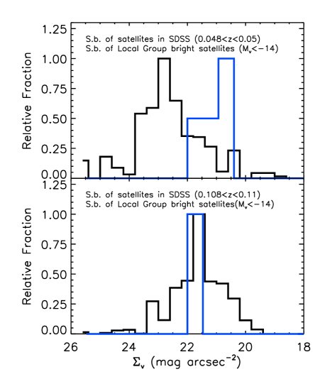
Figure 6: A test of surface brightness effects. The black histograms show the distribution of surface brightnesses, defined as the average surface brightness within the half light radius, for potential satellite galaxies around primaries at redshift $z\approx 0.05$ (upper panel) and $z\approx 0.1$ (lower panel). These are compared with the surface brightness distribution (blue histograms) of those bright Local Group satellites which would be brighter than our $m_{V}=20.5$ apparent magnitude limit when placed at the redshift of the selected primaries. These equivalent surface brightnesses, computed from the data provided by Mateo (1998), have been k-corrected and redshift-dimmed to the redshift of the selected primaries.

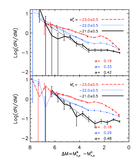
Figure 7: The estimated satellite LFs for different bins of primary magnitude as indicated in the legend. The top panel is for the $V$-band and the bottom panel for the $r$-band. The straight lines show power-law fits to the faint ends of the luminosity functions. Their slopes, $\alpha$, are given in the legend. Here, the selection parameters, $\{R_{\rm{inner}},R_{\rm{outer}},\Delta M_{\rm{bin}},\Delta M_{\rm{faint}},\Delta z_{\rm{s}},\alpha_{\rm{p}}\}$, are set to the default values $\{0.3~{}\rm{Mpc},0.6~{}\rm{Mpc},0.5,0.5,0.002,2.5\}$

.

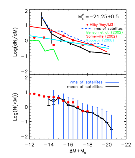
Figure 8: A comparison of the average satellite LF in our sample with the satellite LF of the Milky Way and M31. The upper panel shows the differential satellite LF of MW-like galaxies. The solid line with error bars shows the estimated $V$-band satellite LF of primaries with similar magnitudes to the Milky-Way and M31 ($M_{\rm{c}}=-21.25\pm 0.5$ in the $V$-band). This is compared to the mean LF of the MW and M31 (per central galaxy) in unit magnitude bins shown by the red points. The best fit power law, $dN/dM_{v}=10\times 10^{0.1(M_{v}+5)}$, of Koposov et al. (2008) is shown as the cyan line. The theoretical predictions of Benson et al. (2002) and Somerville (2002) for $z_{\rm{reion}}=10$ are shown by the green and red lines respectively. The blue dashed line labelled “rms of satellites” shows the mean value plus the rms of the LF among different primaries. The lower panel shows the same results and the observational data in cumulative form. Here, the black error bars give the error on the mean cumulative LF while the much broader blue error bars indicate the intrinsic rms scatter about this mean.

4 Results

We now explore the dependence of the satellite LF on the properties of the primary galaxies. Estimates of the V and $r$-band satellite LF for primaries of magnitude $M_{\rm{c}}=-21,-22$ and $-23$ are shown in Fig. 7. As the luminosity of the primary increases the number of satellites increases at all values of $\Delta M$, and, in addition, the shape of the LF changes. None of the luminosity functions are well fit by Schechter functions, i.e. they are not well described by power laws with exponential cutoffs at the bright end. Instead, there is a tendency for the LFs to become flatter at the bright end and the satellite LFs of the brightest primaries even have a local maximum at $\Delta M=2$. Only at the faint end are the luminosity functions accurately represented by power laws. We show such fits and list their slopes in Fig. 7 . The variety of features in the LFs suggests they will place interesting constraints on formation models.

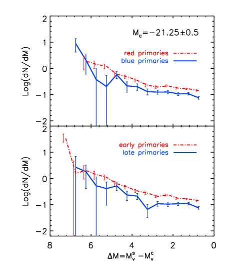
Figure 9: The mean satellite LF of different colours (top panel) and types (bottom panel) of primary galaxy. The satellite LF of early-type or red primary galaxies is shown as a red (dot-dashed) line and that of late-type or blue is plotted as a blue (solid) line.

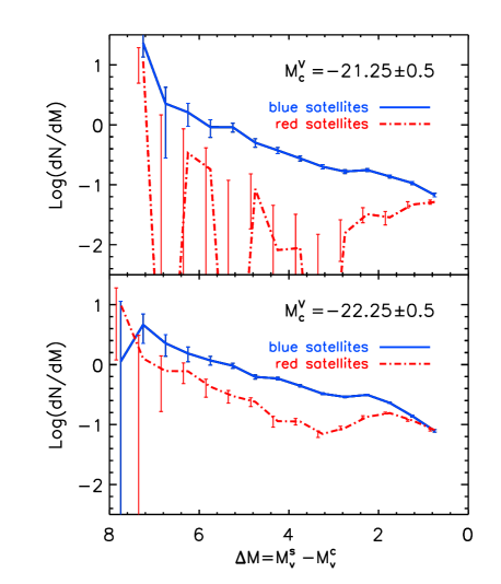
Figure 10: The satellite LF split into contributions from “blue” and “red” satellites. The top and bottom panels show the results for primaries of $V$-band magnitude $M_{\rm{c}}=-21.25$ and $-22.25$ respectively. The “blue” and “red” satellite LFs are plotted as blue (solid) and red (dot-dashed) lines respectively.

In Fig. 8, we carry out a comparison of the satellite LF of primaries of similar luminosity to the MW and M31 with data for these two galaxies. The average satellite LF of the MW and M31 has often been compared to theoretical models (e.g. Benson et al., 2002; Somerville, 2002) and used to constrain properties of the model such as the redshift of reionization and the strength of supernova feedback. In so doing one implicitly assumes that the satellite LF per primary galaxy of the combined MW+M31 system is typical of isolated galaxies of similar luminosity. The data allow a direct test of this assumption at the bright end, $M_{\rm V}<-14$, of the LF. For this comparison, we assume that the $V$-band magnitudes of both the MW and M31 lie in the range $-21.25\pm 0.5$ (Flynn et al., 2006; Gil de Paz et al., 2007) and compare directly with the average of their $V$-band LFs by plotting on the $x$-axis the $V$-band $\Delta M+M_{\rm c}$. Over the range $-14>M_{\rm V}>-19$ our mean LF has a very similar slope to that of the average of the MW and M31, but with almost a factor two fewer satellites at all luminosities. Fainter than $M_{\rm V}=-14$ our estimate becomes noisy due to a lack of nearby primaries. The random errors on our estimate of the mean luminosity density are small at bright magnitudes, yielding a well-defined estimate of the luminosity function that provides a very strong constraint on models all the way to magnitudes as bright as $M_{\rm V}=-20$. Comparison with the theoretical models of Benson et al. (2002) and Somerville (2002) highlights the range of predictions. Tuning the models to match our new data rather than just the MW or M31 may lead to a different assessment of the strength of feedback effects in suppressing the formation of satellite galaxies. This is particularly apparent when one considers the system-to-system variation in the satellite LF. We have estimated the intrinsic rms scatter about the mean LF using the method detailed in the Appendix. We indicate this range with the blue error bars on the cumulative LF in the lower panel of Fig. 8 and the mean plus the rms of the differential LF by the blue dashed line in the upper panel. Since even in the cumulative LF, the mean number of satellites per primary is low it is inevitable that the width of the distribution includes zero satellites. The wide scatter illustrates the danger of just using the MW+M31 to constrain models.

It is also interesting to see how the satellite luminosity function depends on the colour and morphology of the primary galaxy. Fig. 9 shows the resulting satellite LFs when primaries of $V$-band magnitude $-21.25\pm 0.5$ are split by colour and by concentration. In the upper panel we divide the primary galaxies into “red” and “blue” subsamples according to the well-known colour bimodality in the colour-magnitude plane (e.g. Strateva et al., 2001; Baldry et al., 2004; Zehavi et al., 2005). Following Zehavi et al. (2005), we use an equivalent colour criterion of ${}^{0.0}(g-r)_{\rm{cut}}=0.19-0.24M_{r}$ (not identical to Zehavi et al. as our magnitudes are K-corrected to $z=0.0$ rather than $z=0.1$). We see that in this bright satellite regime, the LF around blue primaries is lower than the LF around red primaries. This difference might simply reflect the relative mass of the halos. Assuming stellar mass to correlate with halo mass we would expect that at a fixed $V$-band magnitude blue star forming galaxies would be less massive than their red counterparts.

The lower panel splits the sample into early and late type where the early type is defined as having a concentration index $c\geq 2.6$. This division roughly separates early-type (E/S0) galaxies from late-type (Sa/b/c, Irr) galaxies (Shimasaku et al., 2001). We see that the satellite LF of late types is suppressed with respect to that of the early types. Given the well known correlation between colour and morphology this result is consistent with the division by colour.

We can also use the colour information available in SDSS to probe the properties of the satellites. For two bins of $V$-band primary magnitude, Fig. 10 shows their satellite luminosity functions split into red and blue subsamples using the same cut in the colour magnitude plane as before. We see that at all but the brightest magnitudes the satellites are predominately blue and star forming. This is in stark contrast with the satellites in groups and clusters where the brightest tend to be red and dead while the faintest are blue (Skibba & Sheth, 2009). We also note that the LF of the red satellites is far from a power law. It has a distinct dip in the range from $3.0<\Delta M<5.0$ and, for the brighter primaries, the peak $\Delta M\approx 2.0$ that we noted earlier in the total LFs is clearly present in the red subsample (and also in the blue subsample).

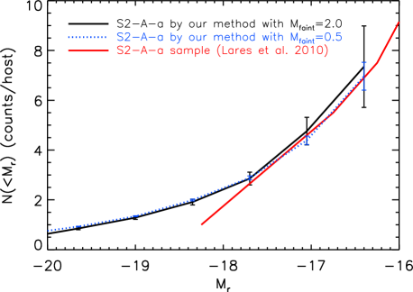
Figure 11: The red line shows the satellite LF estimated by (Lares, Lambas, & Dominguez, 2010) for their S0-A-a subsample. The solid black and dotted blue lines show our result for a similar sample primary galaxies, those brighter than -21.5 in $r$-band and in the redshift range $0.03<z<0.1$, using $\Delta M_{\rm faint}=2.0$ and $0.5$ respectively.

5 Discussion

We have constructed a large sample of isolated primary galaxies and their fainter neighbours using both the SDSS DR7 spectroscopic and photometric galaxy catalogues. The samples are sufficiently large that we are able to stack the systems and accurately subtract the local background to estimate the mean satellite luminosity function (LF) and its dependence on the luminosity, colour and morphology (optical concentration) of the primary. Our main conclusions are:

1. The satellite LF is well determined over a range extending to approximately 8 magnitudes fainter than the primary, for primaries with V magnitudes in the range -20 to -23.

2. The satellite LF does not have a Schechter form. After a steep decline at the faintest magnitudes, the LF roughly follows a fairly flat power law but there is a bump at relative magnitude $\Delta M\simeq 2$ which is particularly significant for brighter primaries (see Fig. 7).

3. Over the range $-14>M_{\rm V}>-19$, the mean satellite LF around primaries of $M_{\rm V}=-21.25$ has a similar slope, but about a factor of two lower amplitude than the average of the combined MW and M31 LFs (see Fig. 8).

4. The amplitude of the satellite LF increases with the luminosity of the primary. Over most of the range sampled, the increase is approximately a factor of 2 per primary V magnitude, but there are significant variations in the shape of the function for primaries of different luminosity (see Fig. 7).

5. The amplitude of the satellite LF also varies with the colour and the morphological type of the primary. Red primaries have more satellites than blue primaries and early-type primaries have more satellites that late-type primaries (see Fig. 9).

6. Except for the brightest objects, satellite galaxies are predominantly blue and star-forming (see Fig. 10).

As we were completing this work two related studies were published, both using the SDSS DR7. Liu et al. (2010) used similar selection criteria to ours to construct a sample of Milky Way-like primaries and deconvolved for the variation of the background to determine the frequency at which these Milky-Way like systems host satellites as bright as the SMC and LMC. They find that 11.6% host one such satellite and only 3.5% host two. And they find a mean of 0.29 satellites per primary. This is in excellent agreement with the mean of 0.30 that we find for satellites between 2 and 4 magnitudes (the range used by Liu et al.) fainter than primaries with the magnitude, $M_{\rm V}=-20.9$, adopted by Liu et al. For the fiducial “Milky Way” luminosity we have adopted here, $M_{\rm V}=-21.25\pm 0.5$, we find a slighly larger mean of 0.47 Magellanic cloud type satellites per primary.

In a separate study, Lares, Lambas, & Dominguez (2010) estimated cumulative satellite luminosity functions and radial density profiles of satellite systems around primaries brighter than $M_{r}=-20.5$. When we reproduce the selection criteria of one of their samples using our catalogue, we find excellent agreement for satellite magnitudes fainter than $M_{r}=-18.5$, but at brighter magnitudes we find a significant excess compared to their estimate (see Fig. 12). This excess is robust to changes in the value of the isolation parameter, $\Delta M_{\rm faint}$, that we have used.

The satellite LF probes the smallest scales visible today in the hierarchy of galaxy formation. This statistic provides a strong test of the $\rm{\Lambda CDM}$ cosmological model, which robustly predicts the number of subhalos that could host satellite galaxies, and a test of galaxy formation theory, which determines which of these subhalos are populated by visible satellites. The results so far are encouraging. For example, the original $\rm{\Lambda CDM}$ galaxy formation model of Benson et al. (2002) (which predicted the population of ultrafaint satellites subsequently discovered in the SDSS), as well as the more recent model of Guo et al. (2010) predict that bright satellites like the LMC and the SMC should be rare. This feature appeared to be a shortcoming of the model when data were available only for the MW (Koposov et al., 2008). The new results for large samples of MW-like galaxies by Liu et al. (2010) and ourselves now suggest that the MW is unusual in having such bright satellites.

According to standard theory, the satellite LF is established by processes that regulate star formation in small halos, namely photoionization of the gas at high redshift and supernova feedback, acting on a population of dark matter subhalos, itself the result of dynamical evolution from a spectrum of primoridal $\rm{\Lambda CDM}$ density perturbations. Our analysis and those by Liu et al. (2010) and Lares, Lambas, & Dominguez (2010) reveal features in the satellite LF and systematic trends with the properties of the central galaxies. These properties encode information about galaxy formation processes that will help develop increasingly refined theoretical models.

Appendix A Estimate of the population variance

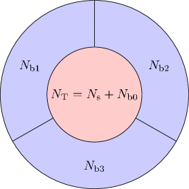
Figure 12: Schematic of the definition of quantities used in the estimation of the population variance. The number of genuine satellites is $N_{\rm s}$ and the number of contaminating background galaxies in the inner area is $N_{\rm b0}$; the number of background galaxies in three equal area regions of the outer annulus are $\langle N_{{\rm b}i}\rangle$, with $i=1,2$ or $3$.

Here we describe the method by which we estimate the intrinsic variance in the number of satellites per primary. As illustrated in Fig. 12 we are only able directly to count the total number of galaxies,

$$N_{\rm T}=N_{\rm s}+N_{\rm b0},$$ (4)

where $N_{\rm s}$ is the number of genuine satellites and $N_{\rm b0}$ is the number of contaminating background galaxies in the inner area. These two contributions cannot be measured separately, but we can estimate the mean number of satellites as,

$$\langle N_{\rm s}\rangle = \langle N_{\rm T}\rangle-\langle N_{\rm b0}\rangle$$ (5)

$$= \langle N_{\rm T}\rangle-f\langle N_{\rm out}\rangle,$$ (6)

where $N_{\rm out}=N_{\rm b1}+N_{\rm b2}+N_{\rm b3}$ is the total number of background galaxies in the outer area and $f$ is the ratio of the inner to outer areas. Below we will take $f=1/3$ which is the case for our default choice of $R_{\rm outer}=2R_{\rm inner}$.

Here we are interested in calculating the variance in the number of satellites, $\langle(N_{\rm s}-\langle N_{\rm s}\rangle)^{2}\rangle$. Starting with equation (4) we can write the variance in the total number of galaxies as

$$\langle(N_{\rm T}-\langle N_{\rm T}\rangle)^{2}\rangle=\langle(N_{\rm s}+N_{\rm b0}-\langle(N_{\rm s}+N_{\rm b0})\rangle)^{2}\rangle$$

$$=\langle(N_{\rm s}-\langle N_{\rm s}\rangle)^{2}\rangle+\langle(N_{\rm b0}-\langle N_{\rm b0}\rangle)^{2}\rangle$$

$$+2\langle(N_{\rm s}-\langle N_{\rm s}\rangle)(N_{\rm b0}-\langle N_{\rm b0}\rangle)\rangle.$$ (7)

If we assume that the number of actual satellites, $N_{\rm s}$, around each primary is uncorrelated with the number of background galaxies, $N_{\rm b0}$, the final cross term vanishes to leave

$$\langle(N_{\rm s}-\langle N_{\rm s}\rangle)^{2}\rangle=\langle(N_{\rm T}-\langle N_{\rm T}\rangle)^{2}\rangle-\langle(N_{\rm b0}-\langle N_{\rm b0}\rangle)^{2}\rangle.$$ (8)

The term, $\langle(N_{\rm b0}-\langle N_{\rm b0}\rangle)^{2}\rangle$ cannot be directly measured, but, to a good approximation, we would expect it to equal the variances, $\langle(N_{{\rm b}i}-\langle N_{{\rm b}i}\rangle)^{2}\rangle$, of each of the equal area portions of the outer annulus. Hence, our final estimate of the variance in the number of genuine satellites per primary can be written as

$$\langle(N_{\rm s}-\langle N_{\rm s}\rangle)^{2}\rangle=\langle(N_{\rm T}-\langle N_{\rm T}\rangle)^{2}\rangle-\frac{1}{3}\sum_{i=1}^{3}\langle(N_{{\rm b}i}-\langle N_{{\rm b}i}\rangle)^{2}\rangle.$$ (9)

For a given selection of primaries and choice of satellite absolute magnitude, these terms will depend on the redshift of the primary. We find a smooth variation with redshift bin and weight the variances according to the contribution each redshift makes to the overall estimate of the satellite luminosity function to estimate the overall variance on the luminosity function. The result is shown in Fig. 8.

References

- (1)
- Abazajian et al. (2009) Abazajian K. N., et al., 2009, ApJS, 182, 543
- Agustsson & Brainerd (2010) Agustsson I., Brainerd T. G., 2010, ApJ, 709, 1321
- Azzaro et al. (2007) Azzaro M., Patiri S. G., Prada F., Zentner A. R., 2007, MNRAS, 376, L43
- Baldry et al. (2004) Baldry I. K., Glazebrook K., Brinkmann J., Ivezić Ž., Lupton R. H., Nichol R. C., Szalay A. S., 2004, ApJ, 600, 681
- Belokurov et al. (2008) Belokurov V., Walker M. G., Evans N. W., et al., 2008, ApJ, 686, L83 08
- Belokurov et al. (2010) Belokurov V., Walker M. G., Evans N. W., et al., 2010, ArXiv e-prints
- Benson et al. (2002) Benson, A. J., Frenk, C. S., Lacey, C. G., Baugh, C. M., & Cole, S. 2002, MNRAS, 333, 177
- Blanton & Roweis (2007) Blanton M. R., Roweis S., 2007, AJ, 133, 734
- Bode, Ostriker, & Turok (2001) Bode P., Ostriker J. P., Turok N., 2001, ApJ, 556, 93
- Boylan-Kolchin et al. (2010) Boylan-Kolchin M., Springel V., White S. D. M., Jenkins A., 2010, MNRAS, 406, 896
- Bullock, Kravtsov & Weinberg (2000) Bullock, J. S., Kravtsov, A. V. & Weinberg, D. H.2000, ApJ, 539, 517
- Busha et al. (2010) Busha M. T., Alvarez M. A., Wechsler R. H., Abel T., Strigari L. E., 2010, ApJ, 710, 408
- Chen et al. (2006) Chen J., Kravtsov A. V., Prada F., Sheldon E. S., Klypin A. A., Blanton M. R., Brinkmann J., Thakar A. R., 2006, ApJ, 647, 86
- Cooper et al. (2010) Cooper A. P., et al., 2010, MNRAS, 406, 744
- Colless et al. (2001) Colless M., et al., 2001, MNRAS, 328, 1039
- Collins et al. (2010) Collins M. L. M., et al., 2010, MNRAS, 407, 2411
- Craig & Davis (2001) Craig M. W., Davis M., 2001, NewA, 6, 425
- Diemand, Kuhlen & Madau (2007) Diemand, J., Kuhlen, M., Madau, P. 2007, ApJ, 657, 262
- Driver et al. (2005) Driver S. P., Liske J., Cross N. J. G., De Propris R., Allen P. D., 2005, MNRAS, 360, 81
- Flynn et al. (2006) Flynn C., Holmberg J., Portinari L., Fuchs B., Jahreiß H., 2006, MNRAS, 372, 1149
- Font et al. (2011) Font A. S., et al., 2011, arXiv, arXiv:1103.0024
- Gil de Paz et al. (2007) Gil de Paz, A., et al. 2007, ApJS, 173, 185
- Guo et al. (2010) Guo Q., et al., 2010, arXiv, arXiv:1006.0106
- Klypin et al. (1999) Klypin, A., Kravtsov, A. V., Valenzuela, O., & Prada, F. 1999, ApJ, 522, 82
- Koposov et al. (2008) Koposov, S., et al. 2008, ApJ, 686, 279
- Lovell et al. (2011) Lovell M., et al., 2011, arXiv, arXiv:1104.2929
- Grebel (2000) Grebel E. K., 2000, in Star Formation from the Small to the Large Scale, edited by F. Favata, A. Kaas, A. Wilson, vol. 445 of ESA Special Publication, 87
- Holmberg (1969) Holmberg E., 1969, ArA, 5, 305
- Hwang & Park (2010) Hwang H. S., Park C., 2010, arXiv, arXiv:1007.2051
- Irwin et al. (2007) Irwin M. J., Belokurov V., Evans N. W., et al., 2007, ApJ, 656, L13
- Kauffmann et al. (1993) Kauffmann, G., White, S. D. M., & Guiderdoni, B. 1993, MNRAS, 264, 201
- Koposov et al. (2009) Koposov, S. E., Yoo, J., Rix, H.-W., Weinberg, D. H., Macciò, A. V.; Escudé, J. M. 2009, ApJ, 696, 2179
- Lares, Lambas, & Dominguez (2010) Lares M., Lambas D. G., Dominguez M. J. L., 2010, arXiv, arXiv:1011.5227
- Li, De Lucia, & Helmi (2010) Li Y.-S., De Lucia G., Helmi A., 2010, MNRAS, 401, 2036
- Libeskind et al. (2007) Libeskind, N. I., Cole, S., Frenk, C. S., Okamoto, T., Jenkins, A. 2007, MNRAS, 374, 16L
- Liu et al. (2008) Liu C., Hu J., Newberg H., Zhao Y., 2008, A&A, 477, 139
- Liu et al. (2010) Liu L., Gerke B. F., Wechsler R. H., Behroozi P. S., Busha M. T., 2010, arXiv, arXiv:1011.2255
- Lorrimer et al. (1994) Lorrimer S. J., Frenk C. S., Smith R. M., White S. D. M., Zaritsky D., 1994, MNRAS, 269, 696
- Macciò et al. (2010) Macciò A. V., Kang X., Fontanot F., Somerville R. S., Koposov S., Monaco P., 2010, MNRAS, 402, 1995
- Martin et al. (2006) Martin, N. F., Ibata, R. A., Irwin, M. J., Chapman, S., Lewis, G. F., Ferguson, A. M. N., Tanvir, N., & McConnachie, A. W. 2006, MNRAS, 371, 1983
- Martin et al. (2008) Martin N. F., de Jong J. T. A., Rix H.-W., 2008, ApJ, 684, 1075
- Mateo (1998) Mateo, M. L. 1998, ARA&A, 36, 435
- Tollerud et al. (2008) Tollerud, E. J., Bullock, J. S., Strigari, L. E., & Willman, B. 2008, ApJ, 688, 277
- McConnachie & Irwin (2006) McConnachie A. W., Irwin M. J., 2006, MNRAS, 365, 1263
- Moore et al. (1999) Moore, B., Ghigna, S., Governato, F., Lake, G., Quinn, T., Stadel, J., & Tozzi, P. 1999, ApJ, 524, L19
- Moore et al. (2000) Moore B., Gelato S., Jenkins A., Pearce F. R., Quilis V., 2000, ApJ, 535, L21
- Muñoz et al. (2009) Muñoz, J. A., Madau, P. Loeb, A., Diemand, J. 2009, MNRAS, 400, 1593
- Norberg et al. (2011) Norberg, P. et al. 2011, MNRAS, submitted.
- Okamoto & Frenk (2009) Okamoto T., Frenk C. S., 2009, MNRAS, 399, L174
- Okamoto et al. (2010) Okamoto, T., Frenk, C. S., Jenkins, A., & Theuns, T. 2010, MNRAS, 406, 208
- Sales & Lambas (2004) Sales L., Lambas D. G., 2004, MNRAS, 348, 1236
- Shimasaku et al. (2001) Shimasaku K., et al., 2001, AJ, 122, 1238
- Skibba & Sheth (2009) Skibba R. A., Sheth R. K., 2009, MNRAS, 392, 1080
- Simon & Geha (2007) Simon J. D., Geha M., 2007, ApJ, 670, 313
- Smith et al. (2002) Smith J. A., et al., 2002, AJ, 123, 2121
- Somerville (2002) Somerville, R. S. 2002, ApJ, 572, L23
- Spergel & Steinhardt (2000) Spergel D. N., Steinhardt P. J., 2000, PhRvL, 84, 3760
- Strateva et al. (2001) Strateva I., et al., 2001, AJ, 122, 1861
- Strauss et al. (2001) Strauss M. A., et al., 2002, AJ, 124, 1810
- Springel et al. (2008) Springel, V., et al. 2008, MNRAS, 391, 1685
- Tollerud et al. (2008) Tollerud E. J., Bullock J. S., Strigari L. E., Willman B., 2008, ApJ, 688, 277
- van den Bergh (2000) van den Bergh S., 2000, The galaxies of the Local Group, Cambridge Univ. Press, Cambridge
- Wadepuhl & Springel (2010) Wadepuhl M., Springel V., 2010, arXiv, arXiv:1004.3217
- Watkins et al. (2009) Watkins L. L., Evans N. W., Belokurov V., et al., 2009, MNRAS, 398, 1757
- Yang et al. (2006) Yang X., van den Bosch F. C., Mo H. J., Mao S., Kang X., Weinmann S. M., Guo Y., Jing Y. P., 2006, MNRAS, 369, 1293
- Yang et al. (2007) Yang, X., Mo, H. J., van den Bosch, F. C., Pasquali, A., Li, C., & Barden, M. 2007, ApJ, 671, 153
- York et al. (2000) York D. G., et al., 2000, AJ, 120, 1579
- Yoshida et al. (2000) Yoshida N., Springel V., White S. D. M., Tormen G., 2000, ApJ, 544, L87
- Zaritsky et al. (1993) Zaritsky D., Smith R., Frenk C., White S. D. M., 1993, ApJ, 405, 464
- Zaritsky et al. (1997a) Zaritsky D., Smith R., Frenk C. S., White S. D. M., 1997a, ApJ, 478, L53
- Zaritsky et al. (1997b) Zaritsky D., Smith R., Frenk C., White S. D. M., 1997b, ApJ, 478, 39
- Zehavi et al. (2005) Zehavi I., et al., 2005, ApJ, 630, 1
- Zucker et al. (2007) Zucker D. B., et al., 2007, ApJ, 659, L21
- Zucker et al. (2006) Zucker D. B., et al., 2006, ApJ, 643, L103
- Zucker et al. (2004) Zucker D. B., et al., 2004, ApJ, 612, L121