Period-doubling-bifurcation readout for a Josephson qubit

Abstract

We propose a threshold detector with an operation principle, based on a parametric period-doubling bifurcation in an externally pumped nonlinear resonance circuit. The ac-driven resonance circuit includes a dc-current-biased Josephson junction ensuring parametric frequency conversion (period-doubling bifurcation) due to its quadratic nonlinearity. A sharp onset of oscillations at the half-frequency of the drive allows for detection of small variations of an effective inductance and, therefore, the read-out of the quantum state of a coupled Josephson qubit. The bifurcation characteristics of this circuit are compared with those of the conventional Josephson bifurcation amplifier, and its possible advantages are discussed.

The problem of an efficient readout of solid state quantum systems including Josephson qubits (see, e.g., Ref. Makhlin, ) is of high importance from both theoretical and practical points of view. The dispersive readout techniques based on the radio-frequency measurement of reactive electrical parameters (for example, the Josephson inductance Z-Phys-C-JETP or quantum Bloch capacitance Sillanpaa ; Duty ) received significant recognition, since they allow one to minimize the backaction of the readout circuit on a Josephson qubit. Recently, particular interest was focused on such systems operating in the non-linear resonance regime (Duffing oscillator), which was possible due to a cubic non-linearity of the supercurrent in a zero-phase biased Josephson junction Ithier ; Lupascu ; Siddiqi-2006 ; Vijay-2009 . In this regime, under the action of a weak signal and/or fluctuations the circuit undergoes a bifurcation, i.e., a transition between two stable oscillatory states Dykman-80 . The successful idea of application of such a Josephson Bifurcation Amplifier (JBA) for measurements of a qubit was first proposed by Siddiqi et al. Siddiqi-2004 , and this has served for us as a motivation for the development of a readout based on another type of bifurcation in superconducting non-linear circuits.

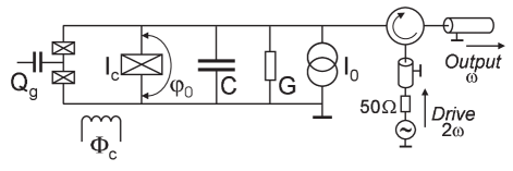
Figure 1: Electric circuit diagram of the period-doubling bifurcation detector with microwave-based readout. The resonator is formed by the inductance of a non-linear Josephson junction (large crossed box), biased at a non-zero phase value $\varphi_{0}$, and the capacitance $C$.
The linear losses are accounted for by the conductance $G$. The resonator is coupled to a charge-phase qubit formed by a superconducting single electron transistor with capacitive gate (left) and attached to the Josephson junction. The qubit operation at the optimal point for an arbitrary bias $I_{0}$ is ensured by a proper value of the external magnetic control flux $\Phi_{c}$, applied to the qubit loop, and the gate charge $Q_{g}$ on the qubit island.

In this paper we propose a readout circuit, whose operation principle is based on excitation of half-harmonic oscillations, i.e., a Period Doubling Bifurcation (PDB), occurring in an rf-driven resonance circuit with quadratic non-linearity of reactance. The essential difference of the PDB from the JBA regime consists in the parametric nature of the PDB resonance manifesting itself in abrupt switching from zero-oscillation state into the dynamic state with a double period and appreciable amplitude of the oscillations Migulin . This regime may be favorable for an output-stage preamplifier receiving in the case of the PDB a signal with zero background. Moreover, as we shall show below, the switching characteristics of our circuits are somewhat different from those of conventional JBA; in particular, we find that in addition to better contrast between two possible stationary states of the PDBA, it may have a narrower switching region.

The PDB circuit (see Fig. 1) comprises a dc-current-biased Josephson junction with the critical current $I_{c}$, capacitance $C$ including the self-capacitance of the junction with, possibly, a contribution of an external capacitance, the linear shunting conductance $G$, as well as an attached qubit, presented here as a charge-phase qubit Vion ; Z-Phys-C-JETP . The circuit is driven by a harmonic signal $I_{\textrm{ac}}=I_{A}\cos 2\omega t$ at a frequency close to the double frequency of small-amplitude plasma oscillations $\omega_{p}$, i.e., $\omega\approx\omega_{p}$.

Neglecting fluctuations, the dynamics of the bare system (excluding the qubit, whose quantum state only slightly changes the plasma frequency of the entire circuit, $\omega_{p}\rightarrow\widetilde{\omega}_{p}$) is governed by the model of a resistively shunted junction RSJ :

$$\frac{\hbar C}{2e}\frac{d^{2}\varphi}{dt^{2}}+\frac{\hbar G}{2e}\frac{d\varphi}{dt}+I_{c}\>\sin\varphi=I_{0}+I_{\textrm{ac}}\,,$$ (1)

where the finite current bias $I_{0}<I_{c}$ ensures a dc phase drop $\varphi_{0}=\arcsin(I_{0}/I_{c})$ across the Josephson junction. The small–ac-signal expansion ($x\ll 1$) of the Josephson supercurrent term includes the following components: $\sin\varphi=\sin(\varphi_{0}+x)\approx\sin\varphi_{0}(1-x^{2}/2+x^{4}/24)+\cos\varphi_{0}(x-x^{3}/6)$. The angular frequency of small oscillations of $\varphi$ around $\varphi_{0}$ is $\omega_{p}=(\cos\varphi_{0})^{1/2}\omega_{p0}$, where the bare plasma frequency is $\omega_{p0}=(2eI_{c}/\hbar C)^{1/2}$.

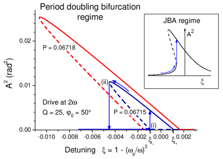
Figure 2: (Color online) Intensity $A^{2}$ of oscillations of the Josephson phase at frequency $\omega$ versus frequency detuning $\xi$ for two amplitudes of the pumping signal (at frequency $2\omega$). Dashed lines show unstable states. When the detuning approaches a bifurcation point ((i) or (ii)), PDB occurs (vertical arrows from or to the zero state, respectively). For comparison, a typical resonance curve of a JBA is sketched in the inset.

Using the dot to denote derivatives with respect to the dimensionless time $\tau=\omega t$, we write the equation of motion for $x$ in the form:

$$\ddot{x}+x=\xi x-2\theta\dot{x}+\beta x^{2}+\gamma x^{3}-\mu x^{4}+3P\,\cos 2\tau.$$ (2)

The dimensionless coefficients in this equation are

$$\xi=1-\kappa\ll 1,\qquad\theta=G/2\omega C\equiv 1/2Q\ll 1,$$ (3)

$$\beta=12\mu=(\kappa\tan\varphi_{0})/2,\quad\gamma=\kappa/6,\quad 3P=\kappa I_{A}/I_{c},$$ (4)

where $\kappa=(\omega_{p}/\omega)^{2}\approx 1$ and $Q$ is the quality factor. The quadratic non-linear term ($\propto\beta$) in Eq. (2) ensures parametric down-conversion from the drive frequency $2\omega$. Note, that similar frequency conversion, and therefore the PDB effect, is also possible without quadratic non-linearity, if instead of the driving force $3P\cos 2\tau$ in Eq. (2) the circuit is parametrically driven by a term of the form $xP^{\prime}\cos 2\tau$ (see, for example, Refs. Migulin, ; Dykman-98, ). This case can be realized by a periodic modulation of the critical current of the zero dc-biased Josephson element $I_{c}$ in a split dc-SQUID configuration by using an alternating magnetic flux driving in the SQUID loop Delsing .

The leading terms in the solution of Eq. (2) have the form $x\equiv y-P\cos 2\tau$, where $y(\tau)$ denotes oscillations at the frequency $\approx\omega$, and the second term is the forced oscillation at the drive frequency $2\omega$; $x(\tau)$ also contains other harmonics at multiple frequencies, which strongly influence its dynamics and stationary states Shteinas , cf. Eqs. (11–12) below. We apply the method of slowly-varying amplitudes by introducing slow variables Migulin ,

$$y=A\cos(\tau-\alpha)\,,\qquad\dot{y}\approx-A\sin(\tau-\alpha)\,.$$ (5)

The variables $A(\tau)$ and $\alpha(\tau)$ present the amplitude and phase (relative to the drive) of the oscillation at the half-frequency of the drive; they vary weakly over the period of these oscillations (with dimensionless rates $\ll 1$). Accordingly,

$$u=A\cos\alpha\,,\qquad v=A\sin\alpha\,$$ (6)

are two quadratures of these oscillations, $u^{2}+v^{2}=A^{2}$. The dynamics of the slow variables is governed by the equations:

$$\left(\begin{array}[]{c}\dot{A}\\ A\dot{\alpha}\end{array}\right)=-\int_{\tau}^{\tau+2\pi}\frac{d\tau}{2\pi}\varepsilon F(x,\dot{x},\tau)\left(\begin{array}[]{c}\sin(\tau-\alpha)\\ \cos(\tau-\alpha)\end{array}\right)\,,$$ (7)

with averaging over a $2\pi$-period of the oscillations at frequency $\omega$ ($1$ in dimensionless units), where the function in the integrand

$$\varepsilon F(x,\dot{x},\tau)=\xi x-2\theta\dot{x}+\beta x^{2}+\gamma x^{3}-\mu x^{4}$$ (8)

includes small terms at frequency $\omega$ and large terms at the drive frequency $2\omega$ and its higher harmonics. The averaging over the period of oscillations in Eq. (7) yields a pair of reduced equations for the amplitude and phase:

$$\dot{A} = -\theta A-\frac{1}{2}A\sin 2\alpha(\tilde{\beta}P-\tilde{\mu}PA^{2})\,,$$ (9)

$$\dot{\alpha} = \frac{\tilde{\xi}}{2}-\frac{\tilde{\beta}P}{2}\cos 2\alpha+\frac{3}{8}\tilde{\gamma}A^{2}+\tilde{\mu}PA^{2}\cos 2\alpha\,.$$ (10)

The coefficients $\tilde{\xi}(P)$, $\tilde{\beta}(P)$, $\tilde{\gamma}(P)$, $\tilde{\mu}(P)$ to the leading order in $P^{2}$ are given by Shteinas

$$\tilde{\xi}=\xi, \tilde{\beta}=\beta,\qquad\tilde{\gamma}=\gamma+\frac{10}{9}\beta^{2},$$ (11)

$$\tilde{\mu} = \mu-\frac{15}{16}\beta\gamma+\frac{7}{24}\beta^{3}\,,$$ (12)

which implies that $\tilde{\gamma}\approx(3+5\tan^{2}\varphi_{0})/18$ and $\tilde{\mu}\approx(7/192)\tan\varphi_{0}(\tan^{2}\varphi_{0}-1)$. Corrections of order $P^{2}$ to these coefficients do not change further analysis qualitatively, but only slightly modify the results quantitatively.

Equation (9) always has a trivial solution $A=0$. In the limit of weak pumping ($P\ll 1$) and small resulting oscillations ($A^{2}\ll 1$), the last terms ($\propto\tilde{\mu}P$) on the right hand side of Eqs. (9–10) can be neglected, and the oscillation amplitude of the non-zero stationary solutions ($\dot{A}=\dot{\alpha}=0$, $A\neq 0$) may be found explicitly Migulin :

$$A_{\pm}^{2}=\frac{4}{3\tilde{\gamma}}\left[-\tilde{\xi}\pm\sqrt{(\tilde{\beta}P)^{2}-4\theta^{2}}\right].$$ (13)

For the pumping amplitude exceeding the threshold set by dissipation, $|\tilde{\beta}P|>2\theta$, the values

$$\tilde{\xi}_{\pm}=\pm\sqrt{(\tilde{\beta}P)^{2}-4\theta^{2}}$$ (14)

yield the range of frequency detunings, $\xi_{-}<\xi<\xi_{+}$, within which the zero solution is unstable. In this range the system switches into the oscillating state with a finite amplitude $A_{+}$ given by Eq. (13). For $\xi<\xi_{-}$ the parametric resonance curve is multivalued with the stable trivial $A=0$ and nontrivial $A_{+}$ solutions, while the solution $A_{-}$ is unstable. Taking into account higher (e.g., $\propto\tilde{\mu}$) terms in Eqs. (9–10) ensures that $A_{+}(\xi)$ and $A_{-}(\xi)$ merge, limiting both the amplitude $A_{+}$ and the the range of bistability in $\xi$; for stronger drive even higher nonlinearities become important. The shape of the resonance curve, calculated numerically from Eqs. (9–10), is shown in Fig. 2 for several values of the drive amplitude $3P$ just above the excitation threshold. However, for further considerations of the threshold behavior the higher nonlinearities are not crucial, and below we neglect the $\tilde{\mu}$-terms.

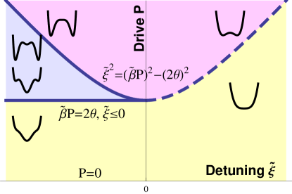
Figure 3: (Color online) Stability diagram of the period-doubling bifurcation readout. Stationary oscillatory solutions appear and disappear as the detuning $\xi$ and driving amplitude $P$ are varied. This is indicated by the sketched potential curves, which show stable (minima) and unstable (maxima) states. The former include: only the zero solution in the lower region, only a pair of equal-amplitude solutions $A_{+}$, $A_{+}^{*}$ with a $\pi$ phase shift in the upper region, and the zero and the pair $A_{+}$, $A_{+}^{*}$ in the left, ‘bistable’ sector-shaped region. The equations in the figure describe the bifurcation boundaries.

The stability diagram of the system in the space of the control parameters, the detuning $\tilde{\xi}$ and the driving amplitude $P$ is shown in Fig. 3. The parameter plane is divided in three regions, with the following stable-state amplitudes (cf. Eq. (13)): $A=0$ in the lower region, $A_{+}$ in the upper region, and both $0$ and $A_{+}$ in the ‘bistable’ sector (this region is limited by two solid lines). The bifurcation lines are given by the relations $A_{+}=A_{-}$ (lower left horizontal solid line), $A_{-}=0$ (i.e., $\xi=\xi_{-}(P)$, upper solid curve) and $A_{+}=0$ (i.e., $\xi=\xi_{+}(P)$, dashed curve). The coordinates of the triple point are $\xi=0$ and $P=2\theta/\tilde{\beta}\approx 2/(Q\tan\varphi_{0})$.

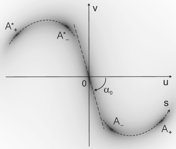
Figure 4: Contour velocity plot calculated from Eqs. (9–10) and (15) for the parameters corresponding to a multivalued solution. The absolute value of velocity $|\textbf{v}|$ is lower in darker areas. The curvilinear trajectory along the valley of minimal velocity (short-dash line) is parametrized by $s$. The straight dashed line at origin indicates the most probable direction of escape from the zero state close to the bifurcation.

Equations for the quadrature components of the velocity field,

$$\textbf{v}=\left(\begin{array}[]{c}\dot{u}\\ \dot{u}\end{array}\right)=\left(\begin{array}[]{c}\dot{A}\cos\alpha-A\dot{\alpha}\sin\alpha\\ \dot{A}\sin\alpha+A\dot{\alpha}\cos\alpha\end{array}\right),$$ (15)

where $\dot{A}$ and $\dot{\alpha}$ are given by (9–10), can be represented as Hamiltonian equations of motion with friction:

$$\dot{u}=-\partial_{v}H-\theta u,\quad\dot{v}=\partial_{u}H-\theta v\,,$$ (16)

or, equivalently,

$$\dot{A}=-\theta A-\frac{1}{A}\partial_{\alpha}H,\quad A\dot{\alpha}=\partial_{A}H\,,$$ (17)

where the Hamiltonian is given by:

$$H=(\tilde{\xi}-\tilde{\beta}P\cos 2\alpha)\frac{A^{2}}{4}+\frac{3}{32}\tilde{\gamma}A^{4}.$$ (18)

This Hamiltonian for the slow variables can be obtained from the Hamiltonian for the physical quantities Shteinas . Figure 4 shows a contour plot of the absolute value of the velocity $|\textbf{v}|=(\dot{u}^{2}+\dot{v}^{2})^{1/2}=(\dot{A}^{2}+A^{2}\dot{\alpha}^{2})^{1/2}$ in the case of a multivalued stationary solution. One can see the darker $S$-shaped narrow valley, where the motion is slow along the curvilinear $s$-axis. The black spots in this area show the stationary solutions, which are the stable focus at zero, $A=0$, the stable foci $A_{+}$ and $A^{*}_{+}$ corresponding to equal-amplitude oscillations with a mutual phase shift of $\pi$, and the unstable saddles $A_{-}$ and $A^{*}_{-}$ (also with a mutual $\pi$-shift). For weak dissipation these ‘saddle points’ are the lower points of the barriers separating the basins of attraction of the foci in the landscape of $H$. Thus the most probable escape path from the zero state is along the $S$-shaped valley.

In the vicinity of the bifurcation point $\xi_{-}$ within the bistable region, the height of the energy barriers is small, and one can show that there is a separation of time scales, which can be used to solve the dynamics: the fast relaxation from outside towards the $S$-shaped valley is followed by slow dynamics along the valley. In this region the points $A_{-}$ and $A^{*}_{-}$ are close to the origin, $u=v=0$, and the slope $\alpha_{0}$ of the valley at the origin can be found from Eq. (9):

$$\sin 2\alpha_{0}=-\eta^{-1},\textrm{\quad where \quad}\eta=\tilde{\beta}P/2\theta.$$ (19)

To describe the slow motion along the valley near the origin, where one can use the amplitude $A$ as a coordinate, we first solve an equation for the fast motion in the axial $\alpha$-direction (variable $\alpha$ relaxes fast, with a typical rate of $\theta$). To find the subleading nonlinear terms in the equation of motion along the valley, one needs to take into account the deviation of the valley near the origin from a straight line. The resulting equation of motion can be represented in the form of an easily solvable 1D equation (cf. Ref. Dykman-80, ):

$$\frac{ds}{d\tau}=-\frac{dW(s)}{ds}\,,$$ (20)

where the pseudopotential is to the lowest orders a biquadratic polynomial, $W=as^{2}-bs^{4}$, where

$$a=-\frac{\delta\tilde{\xi}}{4}\sqrt{\eta^{2}-1}\,,\qquad b=\frac{3}{32}\tilde{\gamma}\sqrt{\eta^{2}-1}\,.$$ (21)

For $\xi<\xi_{-}$ ($\delta\xi<0$) one finds that $a>0$. Thus, when $\xi$ crosses $\xi_{-}$ from above, the zero unstable stationary solution bifurcates and separates into a stable solution at zero and two symmetric unstable solutions $A_{-}$ (Fig. 5). This property makes it sensitive to small changes of the circuit parameters (in particular, to the qubit state via its effective Josephson inductance, which modifies the detuning $\xi$). The switching characteristics of such a detector can be found from the analysis of this system in the presence of noise, which results in a finite width of the transition. To describe the bifurcation-based readout, one needs to find the tunneling rate out of the shallow well $W(s)$ near the bifurcation.

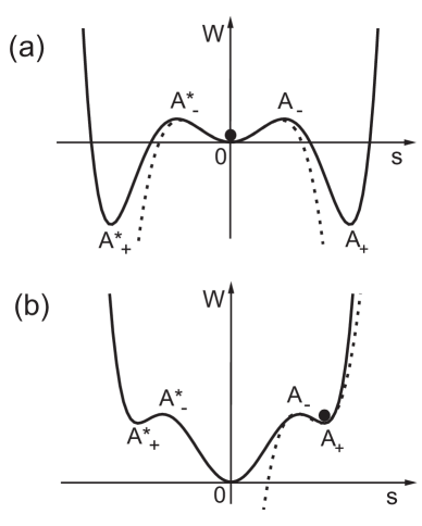
Figure 5: A sketch of the potential $W(s)$ along the $S$-shaped region (see Fig. 4) for two ultimate cases: (a) bifurcation $0\rightarrow A_{+}\,(A^{*}_{+})$ (near the upper solid line in Fig. 3) and (b) bifurcation $A_{+}\rightarrow 0$ (near the lower solid line in Fig. 3). Near the bifurcations the dashed lines approximate the energy barriers by a quartic and cubic polynomials, respectively.

Small fluctuations due to the conductance $G$ are taken into account by adding a noise term $\delta I$, with the spectral density $S_{I}(\omega)=2\hbar\omega G\coth\frac{\hbar\omega}{2k_{B}T}$, to the rhs of Eq. (1). This gives rise to independent fluctuations of the two quadratures. Their correlation functions are

$$\langle\delta u(\tau)\delta u(\tau^{\prime})\rangle=\langle\delta v(\tau)\delta v(\tau^{\prime})\rangle=2T_{\rm eff}\delta(\tau-\tau^{\prime}),$$ (22)

with $\langle\delta u(\tau)\delta v(\tau^{\prime})\rangle=0$ or

$$\langle\delta A(\tau)\delta A(\tau^{\prime})\rangle=A^{2}\langle\delta\alpha(\tau)\delta\alpha(\tau^{\prime})\rangle=2T_{\rm eff}\delta(\tau-\tau^{\prime}),$$ (23)

with $\langle\delta A(\tau)\delta\alpha(\tau^{\prime})\rangle=0$, where the effective temperature

$$T_{\rm eff}=\frac{\kappa^{2}S_{I}(\omega)\omega}{8(I_{c}\cos\varphi_{0})^{2}}\stackrel{{\scriptstyle\mathrm{low-}\omega}}{{\longrightarrow}}\frac{\kappa^{2}k_{B}TG\omega}{2(I_{c}\cos\varphi_{0})^{2}}\,,$$ (24)

and the latter expression holds in the low-frequency (classical) limit $\hbar\omega\ll k_{B}T$. Upon the reduction to the 1D equation (20) this gives fluctuations with the same noise power,

$$\langle\delta s(\tau)\delta s(\tau^{\prime})\rangle=2T_{\rm eff}\delta(\tau-\tau^{\prime})\,,$$ (25)

which affect the motion along the $s$-coordinate.

Adding the Langevin term $\delta s(\tau)$ on the right-hand side of Eq. (20), one can derive and then solve a 1D Fokker-Planck equation Dykman-80 (in fact, a Smoluchowski equation since the ‘mass’ term, $\propto d^{2}s/d\tau^{2}$, is absent in Eq. (20)) for the probability density $w(s,t)$ to find the system at the point $s$ at the time $t$,

$$\frac{\partial w}{\partial t}=\frac{\partial}{\partial s}\left[\frac{\partial W(s)}{\partial s}w\right]+T_{\rm eff}\frac{\partial^{2}w}{\partial s^{2}}\,.$$ (26)

The escape rate out of the zero metastable state $A=0$ to the stable state $A_{+}$ or $A^{*}_{+}$ is given by the Kramers formula Kramers reflecting the activational behavior of the system,

$$\Gamma=2(\omega_{A}/2\pi)e^{-\Delta W/T_{\rm eff}}\,,$$ (27)

where the factor $2$ accounts for two escape possibilities (to the left or right wells). For the overdamped case of a zero-mass particle the formula for $\omega_{A}$ is given, for example, in Ref. Melnikov, . The prefactor $\omega_{A}$ is determined by the geometrical mean of the curvatures of $W(s)$ at the bottom of the central well (equal to $2a$) and at the top of the barrier (equal to $4a$), i.e.,

$$\omega_{A}=2\sqrt{2}a\omega=\omega\frac{|\delta\xi|}{\sqrt{2}}\sqrt{\eta^{2}-1}\,.$$ (28)

The barrier height to the lowest order in $\delta\xi=\xi-\xi_{-}$ is

$$\Delta W=a^{2}/4b\propto(\xi-\xi_{-})^{2}\,.$$ (29)

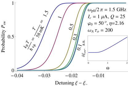
Figure 6: (Color online) Switching curves for the period-doubling bifurcation readout at various temperatures. Note saturation at low $T$, governed by ‘quantum noise’ at $k_{B}T\lesssim\hbar\omega$. Inset: low-$T$ saturation, illustrated by the curves’ width $\delta\xi_{\mathrm{sw}}$ (inverse slope at $P=0.5$, $\propto\sqrt{S(\omega)}$) as a function of $\Theta\equiv\sqrt{k_{B}T/\hbar\omega}$.

Typical switching curves (switching probability $P_{\mathrm{sw}}=1-e^{-\Gamma\tau_{o}}$ during some observation time $\tau_{o}$ vs. $\xi$) are shown in Fig. 6 for various temperatures for a set of typical circuit parameters. Note that the position and the width of the switching curve (see inset) saturates at low temperatures. This effect is not a manifestation of the real quantum tunneling, but is rather linked to the fact that activation in the rotating frame of the first harmonic Eqs. (5,6), i.e., the low-frequency noise in that frame, is given in the laboratory frame by the noise at a finite frequency $\omega$, cf. Eq.(24) and above.

Equation (29) implies that the width (along the detuning axis $\xi$) of the switching curves, given by the inverse slope $(dP/d\xi)^{-1}$ at $P=0.5$, scales as $\delta\xi_{\mathrm{sw}}\propto\sqrt{T}$ above saturation. Thus as $T\rightarrow 0$, it falls off slightly slower than that for the ‘standard’ Josephson bifurcation amplifier Siddiqi-2004 ; Siddiqi-MQC2004 , where $\delta\xi_{\rm sw}\propto T^{2/3}$. This (minor) difference stems from symmetry of the PDBA w.r.t. a shift by a drive period: $\alpha\to\alpha+\pi$. This symmetry implies that the generic form of the 1D potential $W$ near the bifurcation is $\varepsilon s^{2}-as^{4}$ unlike $\varepsilon s-as^{3}$ for the JBA. Here $\varepsilon$ measures the distance from the bifurcation, and $s$ is the relevant coordinate in phase space. However, this symmetry can be broken, and the stronger effect of cooling ($\delta\xi_{\rm sw}\propto T^{2/3}$) restored, by a weak admixture at frequency $\omega$ to the drive signal. An alternative strategy consists in using another bifurcation point, where $A_{+}=A_{-}$ in Fig. 2 (on lowering the detuning $\xi$, the system follows the solution $A_{+}$ until it merges with $A_{-}$, where it switches abruptly to zero; there is no symmetry around this point).

Thus we have suggested two protocols of operation of the PDBA (with potentials shown in Fig. 5 and operation indicated by arrows in the parametric-resonance plot Fig. 2): one of them involves switching from the zero state to a large-amplitude stable state $A_{+}$ near the bifurcation point $\xi_{-}$, and the other involves a reverse switching from the large-amplitude state $A_{+}$ to zero near the merging point of $A_{+}$ and $A_{-}$. Note that in both cases to perform a read-out, that is to find out if a switching has occurred, one needs to distinguish a zero state from a large-amplitude state. This should be contrasted with the JBA, where two finite-amplitude (and often, similar-amplitude, but different-phase) states have to be distinguished. From this viewpoint, the PDBA may be more convenient in practical applications. Other protocols can also be discussed (cf. Ref. Dykman08, ).

The readout of a coupled qubit is based on the shift in the plasma frequency (and thus of the switching curve) due to different Josephson inductances in two qubit states. The inductance values depend on the type of qubit and its parameters. During the readout the qubit state is encoded in the resulting oscillations of the PDBA by tuning the control parameters (such as the drive frequency and amplitude, i.e., $\xi$ and $P$) to a point with the maximal difference (contrast) between the two switching curves. High contrast is reached when the shift in the plasma frequency exceeds the width of the switching curve. In an ideal arrangement, this contrast reaches 100%: $P_{\rm sw}=0$ and $1$ for two qubit states. For the PDBA the contrast reaches values comparable to those for the JBA with similar circuit parameters (for example, about 0.3% in frequency sensitivity for the parameters of Fig. 6 at low $T$, that is sufficient for reliable readout of the charge-phase qubit  Ithier shown in Fig. 1). Further optimization of the PDBA parameters is possible.

Let us compare the switching curves for the PDBA and JBA Ithier near the upper critical lines of the bistability region ($\eta_{\uparrow}$ in the notations of Ref. Ithier, ). We consider the tunneling exponents as functions of the dimensionless deviation of the drive amplitude from the bifurcation, $1-P/P_{-}$, for the PDBA, and we use the same notation, instead of $1-\eta/\eta_{\uparrow}$, for the JBA. According to Refs. Siddiqi-MQC2004, ; Ithier, , for the JBA

$$\left|1-\frac{P}{P_{-}}\right|\sim\left(\frac{k_{\mathrm{B}}T}{E_{J}|\xi|}\right)^{2/3}.$$ (30)

For the PDBA, we replace the difference $(\xi-\xi_{-})$ in Eq. (29) by $\partial_{P}\xi_{-}(P_{-}-P)$. Assuming that the detuning $\xi\gtrsim 1$ (that is $\delta\omega\gtrsim\omega/Q$), we find that the tunneling exponent is of order

$$\frac{\Delta W}{T_{\rm eff}}\approx Q^{2}\frac{6\tilde{\gamma}\cos\varphi_{0}E_{J}}{k_{\mathrm{B}}T}|\xi|^{3}\left(1-\frac{P}{P_{-}}\right)^{2}.$$ (31)

Thus increasing the detuning (and the corresponding driving amplitude $P_{-}(\xi)$) can suppress the width of the relevant switching curve (switching probability-vs.-drive amplitude $P$):

$$\left|1-\frac{P}{P_{-}}\right|\sim\left(\frac{k_{\mathrm{B}}T}{E_{J}|\xi|}\frac{1}{Q^{2}|\xi|^{2}}\frac{1}{6\tilde{\gamma}\cos\varphi_{0}}\right)^{1/2}.$$ (32)

We note that various operation protocols of the readout device based on PDBA are possible, and one can force crossing the bifurcation region and switching between the oscillating states by tuning various parameters. In particular, the current bias $I_{0}$, the amplitude and frequency of the drive can be used for engineering a metapotential of desired shape and, therefore, optimization of the readout. In our analysis we have focused on the noise-induced activation over the barrier in this metapotential. As we saw (cf. above Eq. (24)), the effective ‘temperature’ is set by the noise level at frequency $\omega$ and saturates on lowering the temperature $T$ below $\hbar\omega/k_{B}$. This low-$T$ regime may also be thought of as ‘quantum activation’ MarDyk06 ; Dykman08 . One could also consider the quantum tunneling DmiDyak . However, in similar systems the corresponding tunneling rate is exponentially small, especially close to the bifurcation point (cf. Refs. Dykman08, ; MarDyk06, ).

In conclusion, we have suggested to use a nonlinear Josephson resonator, driven near its double plasma frequency, as a sensitive quantum detector. In this regime the system may develop a bifurcation with two possible stable states; it may be manipulated to force it to the state, correlated with the state of a coupled qubit. In contrast to the Josephson bifurcation amplifier, one of these states has a zero amplitude, which simplifies the task of resolving the two states. Furthermore, the properties of the detector are different from those of the JBA for similar parameters. In particular, the switching curve may be narrower than that for a JBA, that may result in a higher fidelity of the qubit readout.

We thank Michael Wulf, Ralf Dolata and members of the Cluster of Excellence QUEST for useful discussions, and Yuli Nazarov for stimulating comments. This work was partially supported by the EU through the EuroSQIP and SCOPE project, which acknowledges the financial support of the Future and Emerging Technologies (FET) programme within the Seventh Framework Programme for Research of the European Commission, under FET-Open grant number 218783, by DFG (German Science Foundation) through the Grant ZO124/2-1, by RFBR under grant No. 09-02-12282-ofi_m, MES of RF, and the Dynasty foundation (YM).

References

- (1) Yu. Makhlin, G. Schön, and A. Shnirman, Rev. Mod. Phys. 73, 357 (2001).
- (2) A. B. Zorin, Phys. Rev. Lett. 86, 3388 (2001); Physica C (Amsterdam) 368, 284 (2002); Zh. Éksp. i Teor. Fiz. 125, 1423 (2004) [Sov. Phys. JETP 98, 1250 (2004)].
- (3) M. A. Sillanpää, T. Lehtinen, A. Paila, Yu. Makhlin, L. Roschier, P. J. Hakonen, Phys. Rev. Lett. 95, 206806 (2005).
- (4) T. Duty, G. Johansson, K. Bladh, D. Gunnarsson, C. Wilson, P. Delsing, Phys. Rev. Lett. 95, 206807 (2005).
- (5) G. Ithier, Manipulation, readout and analysis of the decoherence of a superconducting quantum bit, PhD thesis, Université Paris 6, 2005.
- (6) I. Siddiqi, R. Vijay, M. Metcalfe, E. Boaknin, L. Frunzio, and M. H. Devoret, Phys. Rev. B 73, 054510 (2006).
- (7) A. Lupaşcu, E. F. C. Driessen, L. Roschier, C. J. P. M. Harmans and J. E. Mooij, Phys. Rev. Lett. 96, 127003 (2006).
- (8) R. Vijay, M. H. Devoret, and I. Siddiqi, Rev. Sci. Instrum. 80, 111101 (2009).
- (9) M. I. Dykman and M. A. Krivoglaz, Physica A 104, 480 (1980).
- (10) I. Siddiqi, R. Vijay, F. Pierre, C. M. Wilson, M. Metcalfe, C. Rigetti, L. Frunzio, and M. H. Devoret, Phys. Rev. Lett. 93, 207002 (2004).
- (11) V. Migulin, V. Medvedev, E. Mustel, and V. Parygin, Basic Theory of Oscillations, V. Migulin, ed. (Mir, Moscow, 1983).
- (12) D. Vion, A. Aassime, A. Cottet, P. Joyez, H. Pothier, C. Urbina, D. Esteve and M. H. Devoret, Science 296, 886 (2002).
- (13) D. E. McCumber, J. Appl. Phys. 39, 3113 (1968); W. C. Stewart, Appl. Phys. Lett. 12, 277 (1968).
- (14) M. I. Dykman, C. M. Maloney, V. N. Smelyanskiy, and M. Silverstein, Phys. Rev. E 57, 5202 (1998).
- (15) C. M. Wilson, T. Duty, M. Sandberg, F. Persson, V. Shumeiko, and P. Delsing, Phys. Rev. Lett. 105, 233907 (2010).
- (16) B. G. Shteinas, Yu. Makhlin, and A. B. Zorin, in preparation.
- (17) A. Dmitriev and M. Dyakonov, Sov. Phys. JETP 63(4), 838 (1986).
- (18) H. A. Kramers, Physica 7, 284 (1940).
- (19) V. I. Mel’nikov, Phys. Rep. 209, 1 (1991).
- (20) M.I. Dykman, in: Applications of Nonlinear Dynamics: Model and Design of Complex Systems, p.367, Springer, 2009 (e-print 0810.5016).
- (21) M. Marthaler, M.I. Dykman, Phys. Rev. A 73, 042108 (2006).
- (22) I. Siddiqi, R. Vijay, F. Pierre, C.M. Wilson, L. Frunzio, M. Metcalfe, C. Rigetti, M.H. Devoret, in: Quantum Computation in Solid State Systems, p. 28, eds. B. Ruggiero, P. Delsing, C. Granata, Y. Pashkin, and P. Silvestrini, Springer, 2006 (e-print: 0507248).