Random walks on Galton–Watson trees with random conductances

Abstract

We consider the random conductance model, where the underlying graph is an infinite supercritical Galton–Watson tree, the conductances are independent but their distribution may depend on the degree of the incident vertices. We prove that, if the mean conductance is finite, there is a deterministic, strictly positive speed $v$ such that $\lim_{n\to\infty}\frac{|X_{n}|}{n}=v$ a.s. (here, $|\cdot|$ stands for the distance from the root). We give a formula for $v$ in terms of the laws of certain effective conductances and show that, if the conductances share the same expected value, the speed is not larger than the speed of simple random walk on Galton–Watson trees. The proof relies on finding a reversible measure for the environment observed by the particle.
Keywords: rate of escape, environment observed by the particle, effective conductance, reversibility
AMS 2000 subject classifications: 60K37, 60J10

${}^{~{}1}$ Technische Universität München, Fakultät für Mathematik, Boltzmannstr. 3, 85748 Garching, Germany
e-mail: gantert@ma.tum.de
url:http://www-m14.ma.tum.de/en/staff/gantert/

${}^{~{}2}$ LATP, CMI Université de Provence 39 rue Joliot Curie, 13453 Marseille cedex 13, France
e-mail: mueller@cmi.univ-mrs.fr,
url:http://www.latp.univ-mrs.fr/$\sim$mueller/

${}^{~{}3}$Department of Statistics, Institute of Mathematics, Statistics and Scientific Computation,
University of Campinas–UNICAMP, rua Sérgio Buarque de Holanda 651, 13083–859, Campinas SP, Brazil
e-mail: {popov,marinav}@ime.unicamp.br,
url: http://www.ime.unicamp.br/$\sim${popov,marinav}

1 Introduction

This paper is a contribution to the theory of random walks on random networks. Here, the underlying graph is an infinite supercritical Galton–Watson tree with independent conductances whose distribution may depend on the degree of the incident vertices. It is not difficult to see that such random walks are transient; see Proposition 2.1. We denote the random walk by $\{X_{n}\}_{n\in{\mathbb{N}}}$. We say that there is a law of large numbers if there exists a deterministic $v$ (the rate of escape, or the speed) such that $\lim_{n\to\infty}\frac{|X_{n}|}{n}=v$ a.s., where, $|\cdot|$ stands for the distance from the root. A standard method to prove laws of large numbers is to work in the space of rooted weighted trees and to consider the environment observed by the particle. This approach has the advantage, provided one is able to construct a stationary measure, that it gives rise to a stationary ergodic Markov chain and one can apply the ergodic theorem. We identify the reversible measure for the environment in Section 3 and prove a formula for the speed which involves effective conductances of subtrees, see Theorem 4.1. A first consequence is that the speed is a.s. positive. For the case of non-degenerate random conductances having the same mean we show a slowdown result: the speed of the random walk with random conductances is strictly smaller than the speed of the simple random walk. Finally, we consider an example on the binary tree, see Proposition 4.5, where explicit asymptotic results are obtained. This example illustrates how the choice of the random environment influences the speed of the random walk.

Simple random walks on Galton–Watson trees were studied in [8] where among other results a law of large number is proved, using the environment observed by the particle. In [10] one finds more references and details about this and related models. There are mainly two generalizations of this model. The first is the so-called $\lambda$-biased random walk. In this model the random walk chooses the direction towards the root with probability proportional to $\lambda$ while the probability to choose any of the sites in the opposite direction is proportional to $1$. In [7] it was proved that the $\lambda$-biased random walk is positive recurrent if $\lambda>m$, null recurrent if $\lambda=m$, and transient otherwise. Here, $m$ is the mean number of offspring of the Galton–Watson process. In the transient case, it was shown in [8] and [9] that $|X_{n}|/n\to v_{\lambda}>0$ a.s., where $v_{\lambda}$ is deterministic. An explicit formula for $v_{\lambda}$ is only known for $\lambda=1$ (that is, for the case of SRW). For $\lambda\leq m$, [11] proves a quenched central limit theorem for $|X_{n}|-nv$ by constructing a stationary measure for the environment process. In the critical case, $\lambda=m$, the central limit theorem has the following form: for almost every realization of the tree, the ratio $|X_{[nt]}|/\sqrt{n}$ converges in law as $n\to\infty$ to a deterministic multiple of the absolute value of a Brownian motion. The second generalization are random walks in random environment (RWRE) on Galton–Watson trees. The main difference to our work is that while in our model the conductances are realizations of an independent environment, in the RWRE model the ratios of the conductances are realizations of an i.i.d. environment. Therefore, the behaviour of RWRE is richer; the walk may be recurrent or transient and the speed positive or zero. We refer to [1] and [6] and references therein for recent results.

Our model can also be seen from a more general point of view as an example of a stationary random network. A stationary random network is a random rooted network whose distribution is invariant under re-rooting along the path of the random walk (defined through the corresponding electric network) started at the original root. This notion generalizes the concept of transitive networks where the condition of transitivity is replaced by the assumption that an invariant distribution along the path of the random walk exists. Under first moment conditions, this model is also known as a unimodular random network, see [3] and [4], or an invariant measure of a graphed equivalence relation. In fact, unimodular random networks correspond to stationary and reversible random networks. A straightforward consequence of the stationarity and the sub-additive ergodic theory, see e.g. [3], is the existence of the speed, i.e., for almost every realization of a stationary and reversible random network, $|X_{n}|/n$ converges almost surely.

The rest of the paper is organized as follows. In Section 2 we give a formal description and notations of the model. The environment observed by the particle is introduced in Section 3 and in Section 4 we present the main results that are proved in Section 5. Some open questions are in Section 6.

2 The model

A rooted tree $T$ is a nonoriented, connected, and locally finite graph without loops. One vertex $\mathbf{o}$ is singled out and called the root of the tree. The rooted tree is then denoted by $(\text{\boldmath$T$},\mathbf{o})$. We use the same notation $T$ for the set of vertices of the tree and the tree itself; the set of edges is denoted by $\mathcal{E}(\text{\boldmath$T$})$. For a vertex $x\in\text{\boldmath$T$}$ we denote by $\mathop{\mathrm{deg}}(x)$ the degree of $x$ (i.e., the number of edges incident to $x$). The index of $x$ is defined by ${\hat{\iota}}(x)=\mathop{\mathrm{deg}}(x)-1$. Let $|x|$ be the (graph) distance from $x$ to the root. We write $x\sim y$ if  $x$ and $y$ are connected by an edge, i.e., $(x,y)\in\mathcal{E}(\text{\boldmath$T$})$. Then, for a fixed tree $T$ and any nonnegative integers $k,m$, define

$$U_{k,m}(\text{\boldmath$T$})= \{(x,y)\in\mathcal{E}(\text{\boldmath$T$}):{\hat{\iota}}(x)=k,{\hat{\iota}}(y)=m\}$$

to be the set of edges connecting vertices of indices $k$ and $m$. An electrical network is a graph where each edge has a positive label called the conductance or weight of the edge. In our model these conductances are realizations of a collection of independent random variables. More precisely, for every unordered pair $\{k,m\}$ we label all edges $e\in U_{k,m}$ with positive i.i.d. random variables $\xi(e)$ with common law ${\tilde{\mu}}_{k,m}$. We denote by $\gamma_{k,m}$ the expected value of $\xi$ under ${\tilde{\mu}}_{k,m}$ (note that $\gamma_{k,m}\in(0,\infty]$ for all $k,m$) and write $\text{\boldmath${\xi}$}:=(\xi(e),~{}e\in\mathcal{E}(\text{\boldmath$T$}))$ for the environment of conductances (weights) on the tree. Clearly, the above definitions are symmetric in the sense that $U_{k,m}(\text{\boldmath$T$})=U_{m,k}(\text{\boldmath$T$})$, ${\tilde{\mu}}_{k,m}={\tilde{\mu}}_{m,k}$, $\gamma_{k,m}=\gamma_{m,k}$ for all $k,m$. Such a weighted rooted tree is then denoted by the triple $(\text{\boldmath$T$},\mathbf{o},\text{\boldmath${\xi}$})$.

Now, we would like to consider a model where the tree itself is chosen at random. Let $p_{0},p_{1},p_{2},p_{3},\ldots$ be the parameters of a Galton–Watson branching process, i.e., $p_{k}$ is the probability that a vertex has $k$ descendants. We assume that $p_{0}=0$, see Remark 4.1 for the case where this assumption is dropped. Furthermore, suppose that

$$\mu:=\sum_{j=1}^{\infty}jp_{j}\in(1,+\infty).$$ (2.1)

The latter guarantees that there exists $j>1$ such that $p_{j}>0$, so that the tree a.s. has infinitely many ends.

Define $\widehat{\mathbb{P}},~{}\widehat{\mathbb{E}}$ to be the probability and expectation for the usual rooted Galton–Watson tree (i.e., the genealogical tree of the Galton–Watson process with the above parameters) with random conductances as described above. Now define $\mathbb{P}_{k,m}$ in the following way, see Figure 1.

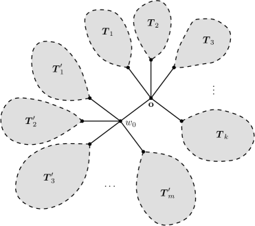
Figure 1: On the definition of $\mathbb{P}_{k,m}$: $\text{\boldmath$T$}_{1},\ldots,\text{\boldmath$T$}_{k}$ and $\text{\boldmath$T$}^{\prime}_{1},\ldots,\text{\boldmath$T$}^{\prime}_{m}$ are i.i.d. weighted Galton–Watson trees with law $\widehat{\mathbb{P}}$

Take i.i.d. copies $\text{\boldmath$T$}_{1},\ldots,\text{\boldmath$T$}_{k},\text{\boldmath$T$}^{\prime}_{1},\ldots,\text{\boldmath$T$}^{\prime}_{m}$ of a weighted Galton–Watson tree with law $\widehat{\mathbb{P}}$. Denote the roots of $\text{\boldmath$T$}_{1},\ldots,\text{\boldmath$T$}_{k}$ by $w_{1},\ldots,w_{k}$. Take a vertex $\mathbf{o}$ with ${\hat{\iota}}(\mathbf{o})=k$ and attach vertices $w_{1},\ldots,w_{k}$ with edges $\ell_{1},\ldots,\ell_{k}$, starting from $\mathbf{o}$. In the same way, attach $\text{\boldmath$T$}^{\prime}_{1},\ldots,\text{\boldmath$T$}^{\prime}_{m}$ to edges starting from a second vertex $w_{0}$. Choose the conductances of all this edges independently according to the corresponding laws. Finally, connect $o$ and $w_{0}$ by an edge and choose its conductance independently from everything according to ${\tilde{\mu}}_{k,m}$. We denote by $\mathbb{E}_{k,m}$ the expectation with respect to $\mathbb{P}_{k,m}$. For each $k$, we can now define $\mathbb{P}_{k}=\sum_{m=1}^{\infty}p_{m}\mathbb{P}_{k,m}$, and we denote by $\mathbb{E}_{k}$ its expectation. Note that $\mathbb{P}_{k}$ is the law of the weighted Galton–Watson tree, conditioned on the event $\{{\hat{\iota}}(\mathbf{o})=k\}$, see Figure 2.

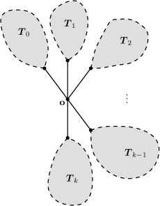
Figure 2: On the definition of $\mathbb{P}_{k}$: $\text{\boldmath$T$}_{0},\ldots,\text{\boldmath$T$}_{k}$ are i.i.d. weighted Galton–Watson trees with law $\widehat{\mathbb{P}}$

Note that with this construction, under $\mathbb{P}_{k}$ the subtrees attached to $w_{0},\ldots,w_{k}$ are independent and have the law $\widehat{\mathbb{P}}$.

The probability measure $\mathbb{P}$ for the augmented Galton–Watson tree with conductances is given by the mixture $\mathbb{P}=\sum_{k=1}^{\infty}p_{k}\mathbb{P}_{k}$. In other words, first we choose an index $k$ with probability $p_{k}$, and then sample the random tree from the measure $\mathbb{P}_{k}$. We note that this is equivalent to considering two independent weighted Galton–Watson trees with law $\widehat{\mathbb{P}}$ connected by a weighted edge; the conductance of this edge is sampled from the corresponding distribution independently of everything. We denote the corresponding expectation by $\mathbb{E}$. The important advantage of considering augmented weighted Galton–Watson trees is the following stationarity property: for any non-negative functions $f,g,u$ on the space of rooted weighted trees we have

$$\mathbb{E}\big{[}f(\text{\boldmath$T$},\mathbf{o},\text{\boldmath${\xi}$})g(\text{\boldmath$T$},w_{0}(\mathbf{o}),\text{\boldmath${\xi}$})u(\xi(\ell_{0}(\mathbf{o})))\big{]}$$

$$=\mathbb{E}\big{[}g(\text{\boldmath$T$},\mathbf{o},\text{\boldmath${\xi}$})f(\text{\boldmath$T$},w_{0}(\mathbf{o}),\text{\boldmath${\xi}$})u(\xi(\ell_{0}(\mathbf{o})))\big{]}.$$ (2.2)

Indeed, using the representation of $\mathbb{E}_{k,m}$ shown in Figure 1, it is straightforward to obtain that

$$\mathbb{E}\big{[}f(\text{\boldmath$T$},\mathbf{o},\text{\boldmath${\xi}$})g(\text{\boldmath$T$},w_{0}(\mathbf{o}),\text{\boldmath${\xi}$})u(\xi(\ell_{0}(\mathbf{o})))\big{]}$$

$$=\sum_{k,m}p_{k}p_{m}\mathbb{E}_{k,m}\big{[}f(\text{\boldmath$T$},\mathbf{o},\text{\boldmath${\xi}$})g(\text{\boldmath$T$},w_{0}(\mathbf{o}),\text{\boldmath${\xi}$})u(\xi(\ell_{0}(\mathbf{o})))\big{]}$$

$$=\sum_{m,k}p_{m}p_{k}\mathbb{E}_{m,k}\big{[}g(\text{\boldmath$T$},\mathbf{o},\text{\boldmath${\xi}$})f(\text{\boldmath$T$},w_{0}(\mathbf{o}),\text{\boldmath${\xi}$}))u(\xi(\ell_{0}(\mathbf{o}))\big{]}$$

$$=\mathbb{E}\big{[}g(\text{\boldmath$T$},\mathbf{o},\text{\boldmath${\xi}$})f(\text{\boldmath$T$},w_{0}(\mathbf{o}),\text{\boldmath${\xi}$})u(\xi(\ell_{0}(\mathbf{o})))\big{]}.$$

Let us denote

$$\pi_{x}=\sum_{z\sim x}\xi(x,z)$$ (2.3)

and define the discrete time random walk $\{X_{n}\}_{n\in{\mathbb{N}}}$ on $T$ in the environment $\text{\boldmath${\omega}$}=(\text{\boldmath$T$},\mathbf{o},\text{\boldmath${\xi}$})$ through the transition probabilities

$$q_{\text{\boldmath${\omega}$}}(x,y)=\frac{\xi(x,y)}{\pi_{x}}.$$

For a fixed realization ${\omega}$ of the environment, denote by ${\mathtt{P}}_{\!\text{\boldmath${\omega}$}},{\mathtt{E}}_{\text{\boldmath${\omega}$}}$ the probability and expectation with respect to the random walk $\{X_{n}\}_{n\in{\mathbb{N}}}$, so that $q_{\text{\boldmath${\omega}$}}(x,y)={\mathtt{P}}_{\!\text{\boldmath${\omega}$}}[X_{n+1}=y\mid X_{n}=x]$ and ${\mathtt{P}}_{\!\text{\boldmath${\omega}$}}[X_{0}=\mathbf{o}]=1$. The definition (2.3) implies that this random walk is reversible with the corresponding reversible measure $\pi$, that is, for all $x,y\in\text{\boldmath$T$}$ we have $\pi_{x}q_{\text{\boldmath${\omega}$}}(x,y)=\pi_{y}q_{\text{\boldmath${\omega}$}}(y,x)=\xi(x,y)$.

It is not difficult to obtain that the random walk defined above is a.s. transient:

Proposition 2.1

The random walk $\{X_{n}\}_{n\in{\mathbb{N}}}$ is transient for $\mathbb{P}$-almost all environments ${\omega}$.

Proof. The random walk is transient if and only if the effective conductance of the tree (from the root to infinity) is strictly positive, see Theorem 2.3 of [10]. By (2.1), we can choose $\delta$ and $d$ such that

$$(1-\delta)\sum_{i=1}^{d}jp_{j}>1.$$ (2.4)

Then, choose $\varepsilon$ small enough such that

$${\tilde{\mu}}_{k,m}[(\varepsilon,\infty)]\geq 1-\delta$$

for all $k,m\leq d$. We define a percolation process on $T$ by deleting all edges with $\xi(e)\leq\varepsilon$. This process dominates a Bernoulli percolation on a $d+1$-regular tree with retention parameter $1-\delta$. Due to (2.4) this percolation process is supercritical. Hence, there is a.s. an infinite subtree of the original tree (not necessarily containing the root) such that all the conductances of this subtree are at least $\varepsilon$. Since this subtree is itself an infinite Galton–Watson tree, the random walk on it is transient and it has positive effective conductance. We conclude that also the effective conductance of the original tree is strictly positive. $\Box$

Remark 2.1

Under the condition that $\gamma=\sum_{k,m}p_{k}p_{m}\gamma_{k,m}<\infty$, Proposition 2.1 is a special case of Proposition 4.10 in [3].

3 Environment observed by the particle

The aim of this section is to construct a reversible measure for the environment, observed by the particle.

Let $\gamma=\sum_{k,m}p_{k}p_{m}\gamma_{k,m}$, and define

$$\mathfrak{m}(\text{\boldmath$T$},\mathbf{o},\text{\boldmath${\xi}$})=\frac{\pi_{\mathbf{o}}}{{\hat{\iota}}(\mathbf{o})+1}$$ (3.1)

Loosely speaking, $\mathfrak{m}$ is the mean conductance from $\mathbf{o}$ to its neighbours. Clearly, we have

$$\mathbb{E}\left(\mathfrak{m}(\text{\boldmath$T$},\mathbf{o},\text{\boldmath${\xi}$})\right)=\sum_{k}\frac{p_{k}}{k+1}\mathbb{E}_{k}(\pi_{\mathbf{o}})=\sum_{k,j}p_{k}p_{j}\gamma_{k,j}=\gamma.$$

Provided that $\gamma<\infty$, we can define a new probability measure $\mathbf{P}$ on the set of weighted rooted trees through the corresponding expectation

$$\mathbf{E}\big{[}f(\text{\boldmath$T$},\mathbf{o},\text{\boldmath${\xi}$})\big{]}=\frac{1}{\gamma}\mathbb{E}\big{[}\mathfrak{m}(\text{\boldmath$T$},\mathbf{o},\text{\boldmath${\xi}$})f(\text{\boldmath$T$},\mathbf{o},\text{\boldmath${\xi}$})\big{]}.$$ (3.2)

Also, for two $\mathbf{P}$-square-integrable functions $f,g$, we define their scalar product

$$(f,g)=\mathbf{E}\big{[}f(\text{\boldmath$T$},\mathbf{o},\text{\boldmath${\xi}$})g(\text{\boldmath$T$},\mathbf{o},\text{\boldmath${\xi}$})\big{]}.$$ (3.3)

The environment observed by the particle is the process on the space of all weighted rooted trees with transition operator

$$Gf(\text{\boldmath$T$},\mathbf{o},\text{\boldmath${\xi}$}) =\sum_{z\sim\mathbf{o}}q_{\text{\boldmath${\omega}$}}(\mathbf{o},z)f(\text{\boldmath$T$},z,\text{\boldmath${\xi}$})$$

$$=\frac{1}{\pi_{\mathbf{o}}}\sum_{z\sim\mathbf{o}}\xi(\mathbf{o},z)f(\text{\boldmath$T$},z,\text{\boldmath${\xi}$}).$$ (3.4)

Let us now prove that $G$ is reversible with respect to $\mathbf{P}$. In particular, this implies that $\mathbf{P}$ is a stationary measure for the environment, observed by the particle.

Lemma 3.1

For any two functions $f,g\in L_{2}(\mathbf{P})$, we have $(f,Gg)=(Gf,g)$.

Proof. Indeed, we have

$$(f,Gg) =\frac{1}{\gamma}\mathbb{E}\Big{[}\frac{1}{{\hat{\iota}}(\mathbf{o})+1}f(\text{\boldmath$T$},\mathbf{o},\text{\boldmath${\xi}$})\sum_{z\sim\mathbf{o}}\xi(\mathbf{o},z)g(\text{\boldmath$T$},z,\text{\boldmath${\xi}$})\Big{]}$$

$$=\frac{1}{\gamma}\sum_{k}\frac{p_{k}}{k+1}\mathbb{E}_{k}\Big{[}f(\text{\boldmath$T$},\mathbf{o},\text{\boldmath${\xi}$})\sum_{j=0}^{k}\xi(\ell_{j}(\mathbf{o}))g(\text{\boldmath$T$},w_{j}(\mathbf{o}),\text{\boldmath${\xi}$})\Big{]}$$

$$=\frac{1}{\gamma}\sum_{k}p_{k}\mathbb{E}_{k}\big{[}f(\text{\boldmath$T$},\mathbf{o},\text{\boldmath${\xi}$})\xi(\ell_{0}(\mathbf{o}))g(\text{\boldmath$T$},w_{0}(\mathbf{o}),\text{\boldmath${\xi}$})\big{]}$$

$$=\frac{1}{\gamma}\mathbb{E}\big{[}f(\text{\boldmath$T$},\mathbf{o},\text{\boldmath${\xi}$})\xi(\ell_{0}(\mathbf{o}))g(\text{\boldmath$T$},w_{0}(\mathbf{o}),\text{\boldmath${\xi}$})\big{]}.$$ (3.5)

In the same way we obtain

$$(g,Gf)=\frac{1}{\gamma}\mathbb{E}\big{[}g(\text{\boldmath$T$},\mathbf{o},\text{\boldmath${\xi}$})\xi(\ell_{0}(\mathbf{o}))f(\text{\boldmath$T$},w_{0}(\mathbf{o}),\text{\boldmath${\xi}$})\big{]},$$ (3.6)

and so, using (2.2), we conclude the proof of Lemma 3.1. $\Box$

4 Main results

Usually, for any weighted rooted tree $(\text{\boldmath$T$},\mathbf{o},\text{\boldmath${\xi}$})$ we will write just $T$ since it is always clear from the context to which root and to which set of weights we are referring. Let ${\mathcal{C}}(\text{\boldmath$T$})$ be the effective conductance from the root to infinity (cf. e.g. Section 2.2 of [10]). Suppose that the random walk starts at the root, i.e., $X_{0}=\mathbf{o}$. Provided that the following limit exists, we define the speed of the random walk $\{X_{n}\}_{n\in{\mathbb{N}}}$ by

$$v=\lim_{n\to\infty}\frac{|X_{n}|}{n}\,.$$ (4.1)

Recall that the neighbours of the root $\mathbf{o}$ are denoted by $w_{0},\ldots,w_{{\hat{\iota}}(\mathbf{o})}$, while $\ell_{0},\ldots,\ell_{{\hat{\iota}}(\mathbf{o})}$ are the corresponding edges. Denote $\xi_{j}:=\xi(\ell_{j})$. Let $\text{\boldmath$T$}_{j}$ be the subtree of $T$ rooted at $w_{j}$ and $\text{\boldmath$T$}_{j}^{*}$ be the tree $\text{\boldmath$T$}_{j}$ together with the edge $\ell_{j}$ (see Figure 3; we assume that the root of $\text{\boldmath$T$}_{j}^{*}$ is $\mathbf{o}$). Note also that

$${\mathcal{C}}(\text{\boldmath$T$}_{j}^{*})=\frac{1}{\frac{1}{\xi_{j}}+\frac{1}{{\mathcal{C}}(\text{\boldmath$T$}_{j})}}.$$ (4.2)

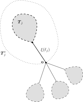
Figure 3: Definition of the tree $\text{\boldmath$T$}_{j}^{*}$

One of the main results of this paper is the following formula for the speed of the random walk with random conductances:

Theorem 4.1

Assume $\gamma<\infty$. Then, the limit in (4.1) exists ${\mathtt{P}}_{\!\text{\boldmath${\omega}$}}$-a.s. for $\mathbb{P}$-almost all $\omega$. Moreover, $v$ is deterministic and is given by

$$v =1-\frac{2}{\gamma}\mathbb{E}\Big{(}\xi_{0}\frac{{\mathcal{C}}(\text{\boldmath$T$}_{0}^{*})}{{\mathcal{C}}(\text{\boldmath$T$})}\Big{)}$$ (4.3)

$$=\sum_{k=1}^{\infty}p_{k}\Big{[}1-\frac{2}{\gamma}\mathbb{E}_{k}\Big{(}\xi_{0}\frac{{\mathcal{C}}(\text{\boldmath$T$}_{0}^{*})}{{\mathcal{C}}(\text{\boldmath$T$})}\Big{)}\Big{]}$$ (4.4)

$$=\sum_{k=1}^{\infty}p_{k}\Big{[}1-\frac{2}{(k+1)\gamma}\mathbb{E}_{k}\Big{(}\sum_{i=0}^{k}\xi_{i}\frac{{\mathcal{C}}(\text{\boldmath$T$}_{i}^{*})}{{\mathcal{C}}(\text{\boldmath$T$})}\Big{)}\Big{]}.$$ (4.5)

Remark 4.1

We can also consider the case when $p_{0}>0$, i.e., when the augmented Galton–Watson process may die out. In this case, we have to condition on the survival of the process. We then obtain the following formula:

$$\lim_{n\to\infty}\frac{|X_{n}|}{n} =1-\frac{2}{\gamma}\mathbb{E}\Big{(}\xi_{0}\frac{{\mathcal{C}}(\text{\boldmath$T$}_{0}^{*})}{{\mathcal{C}}(\text{\boldmath$T$})}\Big{|}survival\Big{)}$$ (4.6)

$$=\sum_{k=1}^{\infty}p_{k}\frac{1-q^{k+1}}{1-q^{2}}\Big{[}1-\frac{2}{\gamma}\mathbb{E}_{k}\Big{(}\xi_{0}\frac{{\mathcal{C}}(\text{\boldmath$T$}_{0}^{*})}{{\mathcal{C}}(\text{\boldmath$T$})}\Big{)}\Big{]},$$ (4.7)

${\mathtt{P}}_{\!\text{\boldmath${\omega}$}}$-a.s. for $\mathbb{P}$-almost all $\omega$, where $q$ is the extinction probability of the Galton–Watson process. The relation of the latter formulas with (4.3) and (4.5) is the same as in [8] for simple random walk.

From (4.3)–(4.5) it is not immediately clear if the speed is positive, so let us prove the following

Theorem 4.2

Assume that $\gamma<\infty$. Then, the quantity $v$ given in (4.3) is strictly positive.

Remark 4.2

In the case of bounded conductances, i.e., if there exists $c,C>0$ such that $\mathop{\rm supp}{\tilde{\mu}}_{k,m}\subseteq[c,C]$, Theorem 4.2 also follows from [12] and the fact that supercritical Galton–Watson trees have the anchored expansion property, see [5].

Next, we treat also the case where the expected conductance in some edges may be infinite:

Theorem 4.3

Assume that there exist $k,m$ such that $\gamma_{k,m}=\infty$. Then, the limit in (4.1) is $0$, ${\mathtt{P}}_{\!\text{\boldmath${\omega}$}}$-a.s. for $\mathbb{P}$-almost all $\omega$.

Using Theorem 4.1, we can compare the speed of the random walk on Galton–Watson trees with random conductances to the speed of simple random walk (SRW) on the same tree (observe that SRW corresponds to the case when all the conductances are a.s. equal to the same positive constant). Let $v_{SRW}$ be the speed of SRW on the Galton–Watson tree; by Theorem 3.2 of [8] it holds that

$$v_{SRW}=\sum_{k}p_{k}\frac{k-1}{k+1}.$$ (4.8)

Theorem 4.4

Assume $\gamma<\infty$. Let $v$ be the speed of the random walk $\{X_{n}\}_{n\in{\mathbb{N}}}$.

• We have

  $$v=v_{SRW}-\frac{2}{\gamma}{\mathop{\rm Cov}}\Big{(}\xi_{0},\frac{{\mathcal{C}}(\text{\boldmath$T$}^{*}_{0})}{{\mathcal{C}}(\text{\boldmath$T$})}\Big{)}$$ (4.9)

  (the covariance is with respect to $\mathbb{E}$).

• Suppose that the conductances have the same expectation, i.e., $\gamma_{k,m}=\gamma$, for all $k,m$, and $\xi_{0}$ is a non-degenerate random variable. Then

  $$v<v_{SRW}.$$ (4.10)

In practice, it is not easy to use Theorem 4.1 for the exact calculation of the speed due to the following reason. While it is not difficult to write a distributional equation that the law of ${\mathcal{C}}(\text{\boldmath$T$}_{0}^{*})$ should satisfy, it is in general not possible to solve this equation explicitly. Nevertheless, Theorem 4.1 can be useful, as the following example shows. Let us consider the binary tree (i.e., $p_{2}=1$) with i.i.d. conductances

$$\xi=\begin{cases}1,&\text{ with probability }1-\varepsilon_{n},\\ a_{n},&\text{ with probability }\varepsilon_{n},\end{cases}$$

where $\varepsilon_{n}\to 0$ and $a_{n}\to\infty$ as $n\to\infty$. Let $v_{n}$ be the speed of the random walk with conductances distributed as above.

Proposition 4.5

Assume that $\varepsilon_{n}a_{n}\to\eta\in[0,\infty]$ as $n\to\infty$. Then,

$$\lim_{n\to\infty}v_{n}=\frac{1}{3(\eta+1)}=\frac{v_{SRW}}{\eta+1}.$$

5 Proofs

Proof of Theorem 4.1. The first part of the proof is to show ergodicity of our process. Since we follow here the arguments in [8], see also [10] (Section 16.3), we only give a sketch. To make use of the ergodic theorem it is convenient to work on the space of bi-infinite paths. A bi-infinite path $\ldots,x_{-1},x_{0},x_{1},\ldots$ is denoted by $\stackrel{{\scriptstyle\leftrightarrow}}{{x}}$. We denote by $\stackrel{{\scriptstyle\rightarrow}}{{x}}$ the path $x_{0},x_{1},\ldots$ and by $\stackrel{{\scriptstyle\leftarrow}}{{x}}$ the path $\ldots,x_{-1},x_{0}.$ The path of the random walk has the property that it converges a.s. to a boundary point; this follows from transience. The space of convergent paths $\stackrel{{\scriptstyle\leftrightarrow}}{{x}}$ in $T$ is denoted by $\stackrel{{\scriptstyle\leftrightarrow}}{{\text{\boldmath$T$}}}$ (convergent means here that one has convergence both for $n\to\infty$ and $n\to-\infty$). We consider the (bi-infinite) path space

$$\textsf{PathsInTrees}:=\left\{(\stackrel{{\scriptstyle\leftrightarrow}}{{x}},\text{\boldmath$T$}):\stackrel{{\scriptstyle\leftrightarrow}}{{x}}\in\stackrel{{\scriptstyle\leftrightarrow}}{{\text{\boldmath$T$}}}\right\}.$$

The rooted tree corresponding to $(\stackrel{{\scriptstyle\leftrightarrow}}{{x}},\text{\boldmath$T$})$ is $(\text{\boldmath$T$},x_{0})$. Define the shift map:

$$(S\!\stackrel{{\scriptstyle\leftrightarrow}}{{x}})_{n}:=x_{n+1},\quad S(\stackrel{{\scriptstyle\leftrightarrow}}{{x}},\text{\boldmath$T$}):=(S\!\stackrel{{\scriptstyle\leftrightarrow}}{{x}},\text{\boldmath$T$})$$

and write $S^{k}$ for the $k$th iteration. In order to define a probability measure on PathsInTrees we extend the random walk to all integers by letting $\stackrel{{\scriptstyle\leftarrow}}{{x}}$ be an independent copy of $\stackrel{{\scriptstyle\rightarrow}}{{x}}$. We use the notation $RW\times\mathbf{P}$ for the corresponding measure on PathsInTrees. Observe that due to the reversibility of the probability measure $\mathbf{P}$ (see Lemma 3.1), the corresponding Markov chain, describing the environment and the path seen from the current position of the walker, is stationary. We proceed by a regeneration argument. Define the set of regeneration points

$$\textsf{Regen}:=\{(\stackrel{{\scriptstyle\leftrightarrow}}{{x}},\text{\boldmath$T$})\in\textsf{PathsInTrees}:x_{-n}\neq x_{0}\text{ and }x_{n}\neq x_{-1}\text{ for all }n>0\}.$$

The first step is to show that a.s. the trajectory has infinitely many regeneration points. To this end, define the set of “fresh” points:

$$\textsf{Fresh}:=\{(\stackrel{{\scriptstyle\leftrightarrow}}{{x}},\text{\boldmath$T$})\in\textsf{PathsInTrees}:x_{n}\neq x_{0}\text{ for all }n<0\}.$$

The idea is to show that the trajectory of the particle a.s. has infinitely many fresh points, and then one concludes by observing that a positive fraction of the fresh points has a (uniform) positive probability to be a regeneration point. The first fact follows from a.s. transience of the random walk and the fact that two independent random walks converge a.s. to different ends. Moreover, there exists a positive density of fresh points. To see this, observe that the sequence $\big{\{}{\mathbf{1}}{\{S^{n}(\stackrel{{\scriptstyle\leftrightarrow}}{{x}},\text{\boldmath$T$})\in\textsf{Fresh}\}},~{}n\in{\mathbb{N}}\big{\}}$ is stationary and hence $\frac{1}{n}\sum_{i=1}^{n}{\mathbf{1}}{\{S^{i}(\stackrel{{\scriptstyle\leftrightarrow}}{{x}},\text{\boldmath$T$})\in\textsf{Fresh}\}}$ converges to some positive (random) number $b$. We define the (a.s. positive) random variable

$$U(\stackrel{{\scriptstyle\leftrightarrow}}{{x}},\text{\boldmath$T$})=\min_{z\sim x_{0}}{\mathtt{P}}_{\!\text{\boldmath${\omega}$}}[X_{1}=z,~{}X_{n}\neq x_{0}\text{ for all }n\geq 1].$$

Again, the sequence $\{{\mathbf{1}}{\{U(S^{n}(\stackrel{{\scriptstyle\leftrightarrow}}{{x}},\text{\boldmath$T$}))>\varepsilon\}},~{}n\in{\mathbb{N}}\}$ is stationary for any $\varepsilon>0$ and we have that $\frac{1}{n}\sum_{i=1}^{n}{\mathbf{1}}{\{U(S^{i}(\stackrel{{\scriptstyle\leftrightarrow}}{{x}},\text{\boldmath$T$}))>\varepsilon\}}$ converges to some (random) $c(\varepsilon)>0$. For every realization of the process (in the bi-infinite path space) we can choose $\varepsilon$ sufficiently small in such a way that $c(\varepsilon)>1-b/2$. Therefore,

$$\liminf_{n\to\infty}\frac{1}{n}\sum_{i=1}^{n}{\mathbf{1}}{\{S^{i}(\stackrel{{\scriptstyle\leftrightarrow}}{{x}},\text{\boldmath$T$})\in\textsf{Fresh}\}}{\mathbf{1}}{\{U(S^{i}(\stackrel{{\scriptstyle\leftrightarrow}}{{x}},\text{\boldmath$T$}))>\varepsilon\}}>b/2.$$

Eventually, this shows the existence of a random sequence $(n_{k})_{k\in{\mathbb{N}}}$ such that $S^{n_{k}}(\stackrel{{\scriptstyle\leftrightarrow}}{{x}},\text{\boldmath$T$})$ is a fresh point and $U(S^{n_{k}}(\stackrel{{\scriptstyle\leftrightarrow}}{{x}},\text{\boldmath$T$}))>\varepsilon$ and hence there exist infinitely many regeneration points. Again we follow the arguments in Section 16.3 of [10]. Let $x$ be some vertex in $T$. We denote by $\text{\boldmath$T$}_{x}$ the subtree of $T$ formed by those edges that become disconnected from $\mathbf{o}$ when $x$ is removed. Define $n_{\textsf{Regen}}=\inf\{n>0:S^{n}(\stackrel{{\scriptstyle\leftrightarrow}}{{x}},\text{\boldmath$T$})\in\textsf{Regen}\}$. To each $(\stackrel{{\scriptstyle\leftrightarrow}}{{x}},\text{\boldmath$T$})\in\textsf{Regen}$ we associate a so-called slab:

$$\textsf{Slab}(\stackrel{{\scriptstyle\leftrightarrow}}{{x}},\text{\boldmath$T$})=(\langle x_{0},x_{1},\ldots,x_{n-1}\rangle,\text{\boldmath$T$}\setminus(\text{\boldmath$T$}^{x_{-1}}\cup\text{\boldmath$T$}^{x_{n}})),$$

where $n=n_{\textsf{Regen}}$ and $\langle x_{0},x_{1},\ldots,x_{n-1}\rangle$ stands for the path of the walk from time $0$ to time $n-1$. Write $S_{\textsf{Regen}}=S^{n_{\textsf{Regen}}}$ when $(\stackrel{{\scriptstyle\leftrightarrow}}{{x}},\text{\boldmath$T$})\in\textsf{Regen}$ and consider the random variables $\textsf{Slab}(S^{k}_{\textsf{Regen}}(\stackrel{{\scriptstyle\leftrightarrow}}{{x}},\text{\boldmath$T$}))$. In contrast to [10] these random variables are not independent. However, if we define $\textsf{Index}(\stackrel{{\scriptstyle\leftrightarrow}}{{x}},\text{\boldmath$T$})={\hat{\iota}}(x_{0})$ then due to the construction of our model we have that $\textsf{Slab}(S^{k}_{\textsf{Regen}}(\stackrel{{\scriptstyle\leftrightarrow}}{{x}},\text{\boldmath$T$}))$ conditioned on $\textsf{Index}(S^{k}_{\textsf{Regen}}(\stackrel{{\scriptstyle\leftrightarrow}}{{x}},\text{\boldmath$T$}))$ is an independent sequence. In order to obtain an i.i.d. sequence we denote by i the smallest possible index, i.e., $\textbf{i}=\inf\{i\geq 1:p_{i}>0\}$ and define

$$\textsf{Regen}_{\textbf{i}}:=\{(\stackrel{{\scriptstyle\leftrightarrow}}{{x}},\text{\boldmath$T$})\in\textsf{Regen}:{\hat{\iota}}(x_{0})=\textbf{i}\}.$$

Since $\textsf{Index}(S^{k}(\stackrel{{\scriptstyle\leftrightarrow}}{{x}},\text{\boldmath$T$}))$ is a stationary Markov chain on $\{i:~{}p_{i}>0\}$ which is irreducible and recurrent one shows that $\textsf{Index}(S^{k}_{\textsf{Regen}}(\stackrel{{\scriptstyle\leftrightarrow}}{{x}},\text{\boldmath$T$}))$ is a recurrent Markov chain. To see this let us first treat the case where $\{i:~{}p_{i}>0\}$ is finite. Then, the probability that $\textsf{Index}(S^{k+1}_{\textsf{Regen}}(\stackrel{{\scriptstyle\leftrightarrow}}{{x}},\text{\boldmath$T$}))=\textbf{i}$ conditioned on $\textsf{Index}(S^{k}_{\textsf{Regen}}(\stackrel{{\scriptstyle\leftrightarrow}}{{x}},\text{\boldmath$T$}))$ is a random variable bounded away from zero. For the general case, we proceed similarly to the proof that there is an infinite number of regeneration points. In fact, we show first that there is a positive fraction of regeneration times. Then, define $V(\stackrel{{\scriptstyle\leftrightarrow}}{{x}},\text{\boldmath$T$})={\hat{\iota}}(\mathbf{o})$ and consider the stationary sequence $\{{\mathbf{1}}{\{V(S^{n}(\stackrel{{\scriptstyle\leftrightarrow}}{{x}},\text{\boldmath$T$})\}\leq K\}},n\in{\mathbb{N}}\}$ for some $K\in{\mathbb{N}}$. Choose $K$ sufficiently large such that there are infinitely many regeneration times whose index is smaller than $K$ and proceed as in the finite case.

Eventually, there is an infinite number of index i regeneration points. Since $\textsf{Slab}(S^{k}_{\textsf{Regen}_{\textbf{i}}}(\stackrel{{\scriptstyle\leftrightarrow}}{{x}},\text{\boldmath$T$}))$ is an i.i.d. sequence that generates the whole tree and the random walk, we obtain that the system $(\textsf{PathsInTrees},RW\times\mathbf{P},S)$ is ergodic.

As in the proof of Theorem 3.2 in [8] we calculate the speed as the increase of the horodistance from a boundary point. So let ${\mathfrak{b}}$ be a boundary point, $x$ be a vertex in $T$, and let us denote by $\mathcal{R}(x,{\mathfrak{b}})$ the ray from $x$ to ${\mathfrak{b}}$. Given two vertices we can define the confluent $x\wedge_{\mathfrak{b}}y$ with respect to ${\mathfrak{b}}$ as the vertex where the two rays $\mathcal{R}(x,{\mathfrak{b}})$ and $\mathcal{R}(y,{\mathfrak{b}})$ coalesce. We define the signed distance from $x$ to $y$ as $[y-x]_{\mathfrak{b}}:=|y-x\wedge_{\mathfrak{b}}y|-|x-x\wedge_{\mathfrak{b}}y|$. (Imagine, you sit in ${\mathfrak{b}}$ and wonder how many steps more you have to do to reach $y$ than to reach $x$.) Denote by $x_{-\infty}$ (respectively, $x_{+\infty}$) the boundary points towards which $\stackrel{{\scriptstyle\leftarrow}}{{x}}$ (respectively, $\stackrel{{\scriptstyle\rightarrow}}{{x}}$) converges. Since $x_{-\infty}\neq x_{+\infty}$ a.s., there exists some constant $c$ such that for all sufficiently large $n$ we have $|x_{n}-x_{0}|=[x_{n}-x_{0}]_{x_{-\infty}}+c$. (More precisely, $c=2|x_{0}-x_{0}\wedge_{x_{\infty}}x_{\infty}|$.) Now, the speed is the limit

$$\lim_{n\to\infty}\frac{1}{n}[x_{n}-x_{0}]_{x_{-\infty}}=\lim_{n\to\infty}\frac{1}{n}\sum_{k=0}^{n-1}[x_{k+1}-x_{k}]_{x_{-\infty}}.$$

Since $(\textsf{PathsInTrees},RW\times\mathbf{P},S)$ is ergodic, these are averages over an ergodic stationary sequence, and hence by the ergodic theorem converge a.s. to their mean

$$v=\int[x_{1}-x_{0}]_{x_{-\infty}}d(RW\times\mathbf{P})(\stackrel{{\scriptstyle\leftrightarrow}}{{x}},\text{\boldmath$T$}).$$ (5.1)

The remaining part of the proof is devoted to find a more explicit expression for this mean. This step is more delicate in the present situation than for SRW. Recall that $\stackrel{{\scriptstyle\leftarrow}}{{x}}$ is an independent copy of $\stackrel{{\scriptstyle\rightarrow}}{{x}}$. Hence, we are interested in the probability that a random walk steps towards the boundary point of a second independent random walk.

We say that the random walk $\{X_{n}\}_{n\in{\mathbb{N}}}$ escapes to infinity in the direction $\ell_{k}$, if

$$|\text{\boldmath$T$}_{k}\cap\{X_{0},X_{1},X_{2},\ldots\}|=\infty.$$

Observe that transience implies that the random walk escapes to infinity in only one direction (since otherwise $\mathbf{o}$ would be visited infinitely many times). Let us define a random variable $\Theta$ in the following way: $\Theta=k$ iff the random walk escapes to infinity in the direction $\ell_{k}$. Let

$$\psi_{\xi}={\mathtt{P}}_{\!\text{\boldmath${\omega}$}}^{\mathbf{o}}[X^{\prime}_{1}=w_{\Theta}(\mathbf{o})]$$

stand for the probability that an independent copy $\{X^{\prime}_{n}\}_{n\in{\mathbb{N}}}$ of the random walk $\{X_{n}\}_{n\in{\mathbb{N}}}$ makes the first step in the escape direction of $\{X_{n}\}_{n\in{\mathbb{N}}}$. Hence, we can write equation (5.1) as

$$v=-\mathbf{E}\psi_{\xi}+\mathbf{E}(1-\psi_{\xi})=1-2\mathbf{E}\psi_{\xi}.$$ (5.2)

Let us compute $\psi_{\xi}$ now.

Claim. We have

$${\mathtt{P}}_{\!\text{\boldmath${\omega}$}}[\Theta=k]=\frac{{\mathcal{C}}(\text{\boldmath$T$}^{*}_{k})}{{\mathcal{C}}(\text{\boldmath$T$})}\,.$$ (5.3)

Proof of the claim. This is, of course, a standard fact, but we still write its proof for completeness. Let

$$\tau_{y}=\inf\{n:X_{n}=y\}.$$

Denote by

$$\eta_{x}(y)={\mathtt{P}}_{\!\text{\boldmath${\omega}$}}^{x}[\tau_{y}=\infty]$$

the probability that the random walk starting from $x$ never hits $y$. Note that

$$\eta_{w_{k}(\mathbf{o})}(\mathbf{o})=\frac{{\mathcal{C}}(\text{\boldmath$T$}_{k}^{*})}{\xi_{k}}=\frac{1}{\xi_{k}}\cdot\frac{1}{\frac{1}{\xi_{k}}+\frac{1}{{\mathcal{C}}(\text{\boldmath$T$}_{k})}}=\frac{{\mathcal{C}}(\text{\boldmath$T$}_{k})}{\xi_{k}+{\mathcal{C}}(\text{\boldmath$T$}_{k})}.$$ (5.4)

This follows e.g. from formula (2.4) of [10] and the fact that, for the random walk with random conductances restricted to $\text{\boldmath$T$}_{k}^{*}$, the escape probability from the root equals $\eta_{w_{k}(\mathbf{o})}(\mathbf{o})$.

Due to the Markov property,

$${\mathtt{P}}_{\!\text{\boldmath${\omega}$}}[\Theta=k] =\frac{\xi_{k}}{\pi_{\mathbf{o}}}\big{(}\eta_{w_{k}(\mathbf{o})}(\mathbf{o})+(1-\eta_{w_{k}(\mathbf{o})}(\mathbf{o})){\mathtt{P}}_{\!\text{\boldmath${\omega}$}}[\Theta=k]\big{)}$$

$$\qquad{}+\sum_{j\neq k}\frac{\xi_{j}}{\pi_{\mathbf{o}}}(1-\eta_{w_{j}(\mathbf{o})}(\mathbf{o})){\mathtt{P}}_{\!\text{\boldmath${\omega}$}}[\Theta=k],$$

so, using (5.4), we obtain

$${\mathtt{P}}_{\!\text{\boldmath${\omega}$}}[\Theta=k] =\Big{(}1-\sum_{j=0}^{{\hat{\iota}}(\mathbf{o})}\frac{\xi_{j}}{\pi_{\mathbf{o}}}\cdot\frac{\xi_{j}}{\xi_{j}+{\mathcal{C}}(\text{\boldmath$T$}_{j})}\Big{)}^{-1}\frac{\xi_{k}}{\pi_{\mathbf{o}}}\cdot\frac{{\mathcal{C}}(\text{\boldmath$T$}_{k})}{\xi_{k}+{\mathcal{C}}(\text{\boldmath$T$}_{k})}$$

$$=\frac{\frac{\xi_{k}}{\pi_{\mathbf{o}}}\cdot\frac{{\mathcal{C}}(\text{\boldmath$T$}_{k})}{\xi_{k}+{\mathcal{C}}(\text{\boldmath$T$}_{k})}}{\sum_{j=0}^{{\hat{\iota}}(\mathbf{o})}\frac{\xi_{j}}{\pi_{\mathbf{o}}}\cdot\frac{{\mathcal{C}}(\text{\boldmath$T$}_{j})}{\xi_{j}+{\mathcal{C}}(\text{\boldmath$T$}_{j})}}$$

$$=\frac{{\mathcal{C}}(\text{\boldmath$T$}^{*}_{k})}{{\mathcal{C}}(\text{\boldmath$T$})},$$

which finishes the proof of the claim. $\Box$

Now, we have

$$\psi_{\xi}=\sum_{k=0}^{{\hat{\iota}}(\mathbf{o})}\frac{\xi_{k}}{\pi_{\mathbf{o}}}{\mathtt{P}}_{\!\text{\boldmath${\omega}$}}[\Theta=k].$$

Then, using (3.2) and plugging in (5.3), we have

$$\mathbf{E}\psi_{\xi} =\mathbf{E}\Big{(}\pi_{\mathbf{o}}^{-1}\frac{\sum_{k=0}^{{\hat{\iota}}(\mathbf{o})}\xi_{k}{\mathcal{C}}(\text{\boldmath$T$}^{*}_{k})}{{\mathcal{C}}(\text{\boldmath$T$})}\Big{)}$$

$$=\sum_{j=1}^{\infty}\frac{p_{j}}{(j+1)\gamma}\mathbb{E}_{j}\Big{(}\frac{\sum_{k=0}^{j}\xi_{k}{\mathcal{C}}(\text{\boldmath$T$}_{k}^{*})}{{\mathcal{C}}(\text{\boldmath$T$})}\Big{)}$$

$$=\sum_{j=1}^{\infty}\frac{p_{j}}{\gamma}\mathbb{E}_{j}\Big{(}\xi_{0}\frac{{\mathcal{C}}(\text{\boldmath$T$}_{0}^{*})}{{\mathcal{C}}(\text{\boldmath$T$})}\Big{)}$$

$$=\frac{1}{\gamma}\mathbb{E}\Big{(}\xi_{0}\frac{{\mathcal{C}}(\text{\boldmath$T$}_{0}^{*})}{{\mathcal{C}}(\text{\boldmath$T$})}\Big{)}.$$

Together with (5.2), this implies (4.3), (4.4), and (4.5). $\Box$

Proof of Theorem 4.2. For each $j$, let $Z_{1}^{(j)},Z_{2}^{(j)},Z_{3}^{(j)},\ldots$ be i.i.d. random variables, having the distribution of the effective conductance of the tree $\text{\boldmath$T$}_{0}^{*}$, conditioned on the event that the root has index $j$. Denote $r_{k,j}=p_{k}p_{j}\gamma_{k,j}/\gamma$; observe that $\sum_{k,j}r_{k,j}=1$, and $r_{k,j}=r_{j,k}$. Assume that $(Z_{i}^{(j)})_{i=1,2,\ldots}$ are independent collections of random variables for $j=1,2,\ldots$. Then we have

$$\sum_{k,j}r_{k,j}E\Big{(}\frac{Z_{1}^{(j)}+\cdots+Z_{j}^{(j)}}{Z_{1}^{(j)}+\cdots+Z_{j}^{(j)}+Z_{1}^{(k)}+\cdots+Z_{k}^{(k)}}\Big{)}$$

$$~{}~{}=\sum_{k,j}r_{k,j}\Big{(}1-E\Big{(}\frac{Z_{1}^{(k)}+\cdots+Z_{k}^{(k)}}{Z_{1}^{(j)}+\cdots+Z_{j}^{(j)}+Z_{1}^{(k)}+\cdots+Z_{k}^{(k)}}\Big{)}\Big{)}$$

$$~{}~{}=1-\sum_{k,j}r_{k,j}E\Big{(}\frac{Z_{1}^{(k)}+\cdots+Z_{k}^{(k)}}{Z_{1}^{(j)}+\cdots+Z_{j}^{(j)}+Z_{1}^{(k)}+\cdots+Z_{k}^{(k)}}\Big{)},$$

so, by symmetry,

$$\sum_{k,j}r_{k,j}E\Big{(}\frac{Z_{1}^{(j)}+\cdots+Z_{j}^{(j)}}{Z_{1}^{(j)}+\cdots+Z_{j}^{(j)}+Z_{1}^{(k)}+\cdots+Z_{k}^{(k)}}\Big{)}=\frac{1}{2}.$$ (5.5)

We have (one may find it helpful to look at Figure 1 again)

$$\mathbb{E}\Big{(}\xi_{0}\frac{{\mathcal{C}}(\text{\boldmath$T$}_{0}^{*})}{{\mathcal{C}}(\text{\boldmath$T$})}\Big{)} =\sum_{k,j}p_{k}p_{j}\mathbb{E}_{k,j}\Big{(}\xi_{0}\frac{{\mathcal{C}}(\text{\boldmath$T$}_{0}^{*})}{{\mathcal{C}}(\text{\boldmath$T$})}\Big{)}$$

$$=\sum_{k,j}p_{k}p_{j}\int\limits_{0}^{\infty}x\mathbb{E}_{k,j}\Big{(}\frac{{\mathcal{C}}(\text{\boldmath$T$}_{0}^{*})}{{\mathcal{C}}(\text{\boldmath$T$})}\mid\xi_{0}=x\Big{)}\,d{\tilde{\mu}}_{k,j}(x)$$

$$<\sum_{k,j}p_{k}p_{j}\int\limits_{0}^{\infty}x\mathbb{E}_{k,j}\Big{(}\frac{{\mathcal{C}}(\text{\boldmath$T$}_{0}^{*})}{{\mathcal{C}}(\text{\boldmath$T$})}\mid\xi_{0}=\infty\Big{)}\,d{\tilde{\mu}}_{k,j}(x)$$

$$=\sum_{k,j}p_{k}p_{j}E\Big{(}\!\frac{Z_{1}^{(j)}+\cdots+Z_{j}^{(j)}}{Z_{1}^{(j)}+\cdots+Z_{j}^{(j)}+Z_{1}^{(k)}+\cdots+Z_{k}^{(k)}}\!\Big{)}\!\int\limits_{0}^{\infty}x\,d{\tilde{\mu}}_{k,j}(x)$$

$$=\gamma\sum_{k,j}r_{k,j}E\Big{(}\frac{Z_{1}^{(j)}+\cdots+Z_{j}^{(j)}}{Z_{1}^{(j)}+\cdots+Z_{j}^{(j)}+Z_{1}^{(k)}+\cdots+Z_{k}^{(k)}}\Big{)}.$$

To see that the inequality in the above calculation is strict, observe that ${\mathcal{C}}(\text{\boldmath$T$})={\mathcal{C}}(\text{\boldmath$T$}_{0}^{*})+\cdots+{\mathcal{C}}(\text{\boldmath$T$}_{k}^{*})$ on $\{{\hat{\iota}}(\mathbf{o})=k\}$, and when the conductance of $w_{0}(\mathbf{o})$ increases, so does the effective conductance of $\text{\boldmath$T$}_{0}^{*}$, and therefore so does the quantity $\frac{{\mathcal{C}}(\text{\boldmath$T$}_{0}^{*})}{{\mathcal{C}}(\text{\boldmath$T$})}$; note also that putting an infinite conductance to an edge means effectively shrinking this edge. Hence, due to (5.5),

$$\mathbb{E}\Big{(}\xi_{0}\frac{{\mathcal{C}}(\text{\boldmath$T$}_{0}^{*})}{{\mathcal{C}}(\text{\boldmath$T$})}\Big{)}<\frac{\gamma}{2}\,.$$ (5.6)

Thus, with (4.3) and (5.6), we obtain $v>0$, which concludes the proof of Theorem 4.2. $\Box$

Proof of Theorem 4.4. Observe that, by symmetry,

$$\mathbb{E}_{k}\Big{(}\frac{{\mathcal{C}}(\text{\boldmath$T$}_{0}^{*})}{{\mathcal{C}}(\text{\boldmath$T$})}\Big{)}=\frac{1}{k+1}.$$ (5.7)

So, from (4.8) we obtain that

$$v_{SRW}=1-\frac{2}{\gamma}\mathbb{E}\left(\xi_{0}\right)\,\mathbb{E}\Big{(}\frac{{\mathcal{C}}(\text{\boldmath$T$}_{0}^{*})}{{\mathcal{C}}(\text{\boldmath$T$})}\Big{)},$$

and (4.9) follows from (4.3). Let us now prove part (ii). From (5.7) we obtain that

$$\sum_{m}p_{m}\mathbb{E}_{k,m}\Big{(}\frac{{\mathcal{C}}(\text{\boldmath$T$}_{0}^{*})}{{\mathcal{C}}(\text{\boldmath$T$})}\Big{)}=\frac{1}{k+1}.$$

Once again, we observe that, when $\xi_{0}$ increases (while fixing the other conductances), so does $\frac{{\mathcal{C}}(\text{\boldmath$T$}_{0}^{*})}{{\mathcal{C}}(\text{\boldmath$T$})}$; this means that $\xi_{0}$ and ${\mathcal{C}}(\text{\boldmath$T$}_{0}^{*})/{\mathcal{C}}(\text{\boldmath$T$})$ are positively correlated under $\mathbb{E}_{k,m}$ (and strictly positively correlated for at least one pair $(k,m)$ in the case when $\xi_{0}$ is a nondegenerate random variable), so we have

$$\mathbb{E}\Big{(}\xi_{0}\frac{{\mathcal{C}}(\text{\boldmath$T$}_{0}^{*})}{{\mathcal{C}}(\text{\boldmath$T$})}\Big{)} =\sum_{k,m}p_{k}p_{m}\mathbb{E}_{k,m}\Big{(}\xi_{0}\frac{{\mathcal{C}}(\text{\boldmath$T$}_{0}^{*})}{{\mathcal{C}}(\text{\boldmath$T$})}\Big{)}$$

$$>\sum_{k,m}p_{k}p_{m}\gamma_{k,m}\mathbb{E}_{k,m}\Big{(}\frac{{\mathcal{C}}(\text{\boldmath$T$}_{0}^{*})}{{\mathcal{C}}(\text{\boldmath$T$})}\Big{)}$$

$$=\gamma\sum_{k}\frac{p_{k}}{k+1}$$

$$=\mathbb{E}\left(\xi_{0}\right)\,\mathbb{E}\Big{(}\frac{{\mathcal{C}}(\text{\boldmath$T$}_{0}^{*})}{{\mathcal{C}}(\text{\boldmath$T$})}\Big{)},$$

where we used $\gamma_{k,m}=\gamma$, for all $k,m$ for the third equality. Now part (ii) follows from (4.9). $\Box$

Proof of Theorem 4.3. Assume that there exist $k,m$ such that $\gamma_{k,m}=\infty$. We will show that for $T_{n}:=\inf\{j:|X_{j}|=n\}$,

$$\frac{T_{n}}{n}\to\infty\quad\text{${\mathtt{P}}_{\!\text{\boldmath${\omega}$}}$-a.s. for $\mathbb{P}$-almost all~{}$\omega$.}$$ (5.8)

Since, for any $\varepsilon>0$, $\{|X_{n}|\geq\lfloor n\varepsilon\rfloor\}\subseteq\{T_{\lfloor n\varepsilon\rfloor}\leq n\}$, (5.8) implies that $\frac{|X_{n}|}{n}\to 0$, ${\mathtt{P}}_{\!\text{\boldmath${\omega}$}}$-a.s. for $\mathbb{P}$-almost all $\omega$. To show (5.8), we will prove that there is an i.i.d. sequence of random variables $(\eta_{j})_{j\geq 1}$ with infinite expectations such that $T_{n}$ is larger than $\frac{1}{\lfloor n/5\rfloor}\sum_{i=1}^{\lfloor n/5\rfloor}\eta_{i}$. Roughly speaking, the infinite expectations come from the fact that the random walk frequently crosses bonds $(y,z)$ with ${\hat{\iota}}(y)=k$ and ${\hat{\iota}}(z)=m$, where the conductances of the neighbouring bonds are not too large. To understand the following proof, it is good to keep in mind that we can construct the tree successively with the random walk, adding new vertices and edges as the random walk explores the tree.

Let $M,C>0$ (to be specified later). For any $x\neq\mathbf{o}$ we denote by $\overleftarrow{x}$ the predecessor vertex with respect to $x$, i.e., $\overleftarrow{x}$ is the neighbor of $x$ such that $|\overleftarrow{x}|=|x|-1$. Let a vertex $x\neq\mathbf{o}$ be good if ${\hat{\iota}}(x)\leq M$, ${\hat{\iota}}(\overleftarrow{x})\leq M$, and $\xi(\overleftarrow{x},x)\leq C$, i.e., the bond from $x$ towards the root has conductance at most $C$, while the degrees of $x$ and its predecessor are not too large.

We now define recursively cutsets of good vertices which the random walk has to cross on its way. For $u,v\in\text{\boldmath$T$}$ with $u<v$, let a “ray from $u$ to $v$” be a path $(z_{1},\ldots,z_{K})$, with $z_{1}=u$ and $|z_{i+1}|=|z_{i}|+1$, $\forall i$ and $z_{K}=v$. Call a vertex bad if it is not good. Let ${\mathcal{G}}_{1}$ be the set of all vertices $u_{1}$ which are good and such that all vertices on the ray from the root to $u_{1}$ are bad. Then, let ${\mathcal{G}}_{2}$ be the set of all vertices $u_{2}$ which are good and such that the ray from the root to $u_{2}$ contains exactly one good vertex $u_{1}\in{\mathcal{G}}_{1}$ with $|u_{1}|<|u_{2}|$, and so on, see Figure 4.

Figure 4: On the definition of the cutsets ${\mathcal{G}}_{1},{\mathcal{G}}_{2},\ldots$ (good sites are marked by larger circles)

Let $B_{n}:=\{u\in\text{\boldmath$T$}:|u|\leq n\}$.

Claim. We can choose large enough $M,C$ in such a way that

$$\mathbb{P}[{\mathcal{G}}_{\lfloor n/5\rfloor}\subseteq B_{n}\hbox{ for all }n\hbox{ large enough}]=1\,.$$ (5.9)

Proof of the claim. If ${\mathcal{G}}_{\lfloor n/5\rfloor}\not\subseteq B_{n}$, there has to be a ray from the root to a vertex at distance $n$ from the root, containing at least $4n/5$ bad vertices; we will show that this happens with exponentially small probability and so one obtains (5.9) from the Borel–Cantelli lemma.

First, let us prove that, for large enough $M$, with large probability on every path to the level $n$ there are at most $n/5$ sites with index greater than $M$. For this, consider a branching random walk starting with one particle at the origin, described in the following way:

• on the first step the particle generates $j+1$ offspring with probabilities $p_{j}$, $j\geq 1$, and on subsequent time moments every particle generates $j$ offspring with probabilities $p_{j}$, $j\geq 1$, independently of the others;

• if the number of a particle’s offspring is less than or equal to $M$, then all the offspring stay on the same place, and if it is greater than $M$, then all its offspring go one unit to the right.

With this interpretation, we have to prove that with large probability at time $n$ the whole cloud is to the left of $n/5$. In fact, it is well-known that the position of the righthmost particle grows linearly in time, and the linear speed goes to $0$ if $M$ goes to $\infty$; there are several possible ways to show this. For instance, one can use the many-to-one lemma (see e.g. formula (2.2) of [2]), dealing with the small difficulty that at time $1$ the offspring distribution is different. Another possibility is to consider the process

$$Z_{n}=(2\mu)^{-n}\sum_{k\in{\mathbb{Z}}}\eta_{n}(k)(2\mu)^{6k},$$

where $\mu=\sum_{j=1}^{\infty}jp_{j}$ and $\eta_{n}(k)$ is the number of particles of the branching random walk at time $n$ at site $k$. With a straightforward calculation, one obtains that if $M$ is large enough, then $Z$ is a (nonnegative) supermartingale. So, we obtain

$$\mathbb{P}[\text{there exists }k\geq n/5\text{ such that }\eta_{n}(k)\geq 1] \leq\mathbb{P}[Z_{n}\geq(2\mu)^{-n}\cdot(2\mu)^{6n/5}]$$

$$\leq\frac{\mathbb{E}Z_{n}}{(2\mu)^{n/5}},$$

$$\leq(2\mu)^{-n/5}\,,$$ (5.10)

using in the last inequality the fact that $Z$ is a supermartingale.

Now, if every path to the level $n$ contains at most $n/5$ sites with index greater than $M$, then on every path to the level $n$ there are at least $3n/5-1$ sites with index less than or equal to $M$ and such the predecessor site has index less than or equal to $M$ as well. Also, using the Chebychev inequality one immediately obtains that with probability at least $1-2^{-n}$ the total number of paths to level $n$ is less than $(2\mu)^{n}$. Next, denoting by

$$h(C)=\max_{i,j\leq M}{\tilde{\mu}}_{i,j}(C,+\infty),$$

we have, clearly, that $h(C)\to 0$ as $C\to\infty$. Let us choose $C$ in such a way that $h(C)$ is small enough to assure the following: on a fixed path to level $n$ (with given degrees of vertices but the conductances not yet chosen) such that the number of bonds there that belong to $\cup_{i,j\leq M}U_{i,j}$ is at least $3n/5-1$, the number of good sites is at least $n/5$ with probability at least $1-(3\mu)^{-n}$ (this amounts to estimating the probability that a sum of $3n/5-1$ Bernoulli random variables with probability of success $1-h(C)$ is at least $n/5$). Then, we use the union bound and the Borel–Cantelli lemma to conclude the proof of the claim. $\Box$

Now, define by ${\tilde{T}}_{j}=\min\{n:X_{n}\in{\mathcal{G}}_{4j}\}$, $k=1,2,3,\ldots$, the hitting times of the sets ${\mathcal{G}}_{4},{\mathcal{G}}_{8},{\mathcal{G}}_{12},\ldots$ (for formal reasons, we also set ${\tilde{T}}_{0}:=0$). Without restricting generality, one can assume that $M\geq\max\{k,m\}$ (recall that $k,m$ are such that $\gamma_{k,m}=\infty$). Consider the events $A_{j}$, $j=1,2,3,\ldots$, defined in the following way:

$$A_{j} =\Big{\{}\text{there exist }y,z\text{ with }{\hat{\iota}}(y)=k,{\hat{\iota}}(z)=m,\text{ such that }y=\overleftarrow{z},X_{{\tilde{T}}_{j}}=\overleftarrow{y},$$

$$~{}~{}~{}~{}~{}~{}~{}\text{ and }C^{-1}\leq\xi(e)\leq C\text{ for all }e\neq(y,z)\text{ such that }e\sim y\text{ or }e\sim z\Big{\}}$$

(observe that the event $A_{j}$ concerns the yet unexplored part of the tree at time ${\tilde{T}}_{j}$). Note that there is some $g=g(M,C)>0$ such that

$$\mathbb{E}{\mathtt{P}}_{\!\omega}[A_{j}]\geq g(M,C)\,.$$ (5.11)

Further, if $X_{{\tilde{T}}_{j}}=x$, then, since $x$ is good, the probability to go from $x$ to $y$ (i.e., the site in the definition of the event $A_{j}$) is bounded below by $\frac{1}{(1+M)C^{2}}$. Then, the number of subsequent crossings $N_{(y,z)}$ of the bond $(y,z)$ (again, $y,z$ are the sites from the definition of the event $A_{j}$) dominates a geometric random variable with parameter $h_{0}:=\frac{(k+m)C}{\xi(y,z)+(k+m)C}$. So, under the averaged measure $\mathbb{E}{\mathtt{P}}_{\!\omega}=\int{\mathtt{P}}_{\!\omega}[\,\cdot\,]\mathbb{P}(d\omega)$, each of the random variables $({\tilde{T}}_{j}-{\tilde{T}}_{j-1})$ dominates a random variable $\eta_{j}$ with law

$$\eta_{j}=\begin{cases}0,&\text{with probability }1-\frac{g(M,C)}{(1+M)C^{2}},\\ \mathsf{Geometric}(h_{0}),&\text{with probability }\frac{g(M,C)}{(1+M)C^{2}},\end{cases}$$

and $\eta_{1},\eta_{2},\eta_{3},\ldots$ are i.i.d. under the measure $\mathbb{E}{\mathtt{P}}_{\!\omega}$. Since, clearly, the expectation of $\eta_{1}$ under the averaged measure $\mathbb{E}{\mathtt{P}}_{\!\omega}$ is infinite, this implies Theorem 4.3 as explained in the beginning of the proof. $\Box$

Proof of Proposition 4.5. For the binary tree, equation (4.3) implies that (see Figure 5)

$$v =1-\frac{2}{\gamma}\mathbb{E}\Big{(}\xi_{0}\frac{{\mathcal{C}}(\text{\boldmath$T$}_{0}^{*})}{{\mathcal{C}}(\text{\boldmath$T$})}\Big{)}$$ (5.12)

$$=1-\frac{2}{\gamma}\mathbb{E}\Big{(}\xi_{0}\frac{\big{(}1+\frac{{\mathcal{C}}(\text{\boldmath$T$}_{00}^{*})+{\mathcal{C}}(\text{\boldmath$T$}_{01}^{*})}{\xi_{0}}\big{)}^{-1}({\mathcal{C}}(\text{\boldmath$T$}_{00}^{*})+{\mathcal{C}}(\text{\boldmath$T$}_{01}^{*}))}{{\mathcal{C}}(\text{\boldmath$T$}_{0}^{*})+{\mathcal{C}}(\text{\boldmath$T$}_{1}^{*})+{\mathcal{C}}(\text{\boldmath$T$}_{2}^{*})}\Big{)}.$$ (5.13)

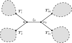
Figure 5: On the definition of the trees $\text{\boldmath$T$}_{00}^{*},\text{\boldmath$T$}_{01}^{*}$

Then, we can write

$$\mathbb{E}\Big{(}\xi_{0}\frac{{\mathcal{C}}(\text{\boldmath$T$}_{0}^{*})}{{\mathcal{C}}(\text{\boldmath$T$})}\Big{)}=(1-\varepsilon_{n})\mathbb{E}\Big{(}\frac{{\mathcal{C}}(\text{\boldmath$T$}_{0}^{*})}{{\mathcal{C}}(\text{\boldmath$T$})}\mid\xi_{0}=1\Big{)}+\varepsilon_{n}a_{n}\mathbb{E}\Big{(}\frac{{\mathcal{C}}(\text{\boldmath$T$}_{0}^{*})}{{\mathcal{C}}(\text{\boldmath$T$})}\mid\xi_{0}=a_{n}\Big{)}.$$ (5.14)

Also, by symmetry we have

$$\frac{1}{3} =\mathbb{E}\left(\frac{{\mathcal{C}}(\text{\boldmath$T$}_{0}^{*})}{{\mathcal{C}}(\text{\boldmath$T$})}\right)$$

$$=(1-\varepsilon_{n})\mathbb{E}\Big{(}\frac{{\mathcal{C}}(\text{\boldmath$T$}_{0}^{*})}{{\mathcal{C}}(\text{\boldmath$T$})}\mid\xi_{0}=1\Big{)}+\varepsilon_{n}\mathbb{E}\Big{(}\frac{{\mathcal{C}}(\text{\boldmath$T$}_{0}^{*})}{{\mathcal{C}}(\text{\boldmath$T$})}\mid\xi_{0}=a_{n}\Big{)}.$$ (5.15)

Since ${\mathcal{C}}(\text{\boldmath$T$}_{0}^{*})/{\mathcal{C}}(\text{\boldmath$T$})\leq 1$, we obtain from (5.15) that

$$\mathbb{E}\Big{(}\frac{{\mathcal{C}}(\text{\boldmath$T$}_{0}^{*})}{{\mathcal{C}}(\text{\boldmath$T$})}\mid\xi_{0}=1\Big{)}\to\frac{1}{3}\qquad\text{as $n\to\infty$}$$ (5.16)

(observe that the expectation in the left-hand side depends on $n$ in fact), and so, by (5.12) and (5.14), we have $v_{n}\to 1-2/3=1/3$ in the case $a_{n}\varepsilon_{n}\to 0$ (note that in this case $\gamma=1-\varepsilon_{n}+a_{n}\varepsilon_{n}\to 1$).

Now we consider the two other cases. First, we want to show that

$$\mathbb{E}\Big{(}\frac{{\mathcal{C}}(\text{\boldmath$T$}_{0}^{*})}{{\mathcal{C}}(\text{\boldmath$T$})}\mid\xi_{0}=a_{n}\Big{)}\to\frac{1}{2}\qquad\text{as $n\to\infty$}.$$

Putting an infinite conductance to the edge $\ell_{0}$, we obtain (as Figure 5 suggests)

$${\mathcal{C}}(\text{\boldmath$T$})<{\mathcal{C}}(\text{\boldmath$T$}_{00}^{*})+{\mathcal{C}}(\text{\boldmath$T$}_{01}^{*})+{\mathcal{C}}(\text{\boldmath$T$}_{1}^{*})+{\mathcal{C}}(\text{\boldmath$T$}_{2}^{*})$$

(naturally, $w_{0}$ is supposed to be the root of $\text{\boldmath$T$}_{00}^{*}$ and $\text{\boldmath$T$}_{01}^{*}$). Then,

$$\mathbb{E}\Big{(}\frac{{\mathcal{C}}(\text{\boldmath$T$}_{0}^{*})}{{\mathcal{C}}(\text{\boldmath$T$})}\mid\xi_{0}=a_{n}\Big{)}$$

$$>\mathbb{E}\Big{(}\frac{{\mathcal{C}}(\text{\boldmath$T$}_{0}^{*})}{{\mathcal{C}}(\text{\boldmath$T$}_{00}^{*})+{\mathcal{C}}(\text{\boldmath$T$}_{01}^{*})+{\mathcal{C}}(\text{\boldmath$T$}_{1}^{*})+{\mathcal{C}}(\text{\boldmath$T$}_{2}^{*})}\mid\xi_{0}=a_{n}\Big{)}$$

$$=\frac{1}{2}-\mathbb{E}\Big{(}\frac{{\mathcal{C}}(\text{\boldmath$T$}_{00}^{*})+{\mathcal{C}}(\text{\boldmath$T$}_{01}^{*})-\big{(}\frac{1}{a_{n}}+\frac{1}{{\mathcal{C}}(\text{\boldmath$T$}_{00}^{*})+{\mathcal{C}}(\text{\boldmath$T$}_{01}^{*})}\big{)}^{-1}}{{\mathcal{C}}(\text{\boldmath$T$}_{00}^{*})+{\mathcal{C}}(\text{\boldmath$T$}_{01}^{*})+{\mathcal{C}}(\text{\boldmath$T$}_{1}^{*})+{\mathcal{C}}(\text{\boldmath$T$}_{2}^{*})}\mid\xi_{0}=a_{n}\Big{)}$$

$$=\frac{1}{2}-\mathbb{E}\Big{(}\frac{{\mathcal{C}}(\text{\boldmath$T$}_{00}^{*})+{\mathcal{C}}(\text{\boldmath$T$}_{01}^{*})}{{\mathcal{C}}(\text{\boldmath$T$}_{00}^{*})+{\mathcal{C}}(\text{\boldmath$T$}_{01}^{*})+{\mathcal{C}}(\text{\boldmath$T$}_{1}^{*})+{\mathcal{C}}(\text{\boldmath$T$}_{2}^{*})}$$

$$\qquad\qquad\qquad\times\Big{[}1-\Big{(}\frac{{\mathcal{C}}(\text{\boldmath$T$}_{00}^{*})+{\mathcal{C}}(\text{\boldmath$T$}_{01}^{*})}{a_{n}}+1\Big{)}^{-1}\Big{]}\Big{)}.$$

Observe that

$$\frac{{\mathcal{C}}(\text{\boldmath$T$}_{00}^{*})+{\mathcal{C}}(\text{\boldmath$T$}_{01}^{*})}{{\mathcal{C}}(\text{\boldmath$T$}_{00}^{*})+{\mathcal{C}}(\text{\boldmath$T$}_{01}^{*})+{\mathcal{C}}(\text{\boldmath$T$}_{1}^{*})+{\mathcal{C}}(\text{\boldmath$T$}_{2}^{*})}<1,$$

and (because if the conductance on the first edge is $1$, then the effective conductance of the tree is less than $1$)

$$\mathbb{P}[{\mathcal{C}}(\text{\boldmath$T$}_{00}^{*})\leq 1]\geq 1-\varepsilon_{n}.$$

Thus, we have that

$$\frac{{\mathcal{C}}(\text{\boldmath$T$}_{00}^{*})+{\mathcal{C}}(\text{\boldmath$T$}_{01}^{*})}{a_{n}}\to 0$$

in probability and so

$$\frac{{\mathcal{C}}(\text{\boldmath$T$}_{00}^{*})+{\mathcal{C}}(\text{\boldmath$T$}_{01}^{*})}{{\mathcal{C}}(\text{\boldmath$T$}_{00}^{*})+{\mathcal{C}}(\text{\boldmath$T$}_{01}^{*})+{\mathcal{C}}(\text{\boldmath$T$}_{1}^{*})+{\mathcal{C}}(\text{\boldmath$T$}_{2}^{*})}\Big{(}1-\Big{(}\frac{{\mathcal{C}}(\text{\boldmath$T$}_{00}^{*})+{\mathcal{C}}(\text{\boldmath$T$}_{01}^{*})}{a_{n}}+1\Big{)}^{-1}\Big{)}\to 0$$

in probability and hence in $L_{1}$. Thus, we indeed have

$$\mathbb{E}\Big{(}\frac{{\mathcal{C}}(\text{\boldmath$T$}_{0}^{*})}{{\mathcal{C}}(\text{\boldmath$T$})}\mid\xi_{0}=a_{n}\Big{)}\to\frac{1}{2}.$$ (5.17)

When $a_{n}\varepsilon_{n}\to\infty$, using (5.14), (5.16), (5.17), we obtain

$$\frac{1}{\gamma}\mathbb{E}\Big{(}\xi_{0}\frac{{\mathcal{C}}(\text{\boldmath$T$}_{0}^{*})}{{\mathcal{C}}(\text{\boldmath$T$})}\Big{)}\to\frac{1}{2}$$

and so $v_{n}\to 0$ by (5.12).

When $a_{n}\varepsilon_{n}\to\eta\in(0,\infty)$, we have by (5.14), (5.16), (5.17), that

$$\frac{1}{\gamma}\mathbb{E}\Big{(}\xi_{0}\frac{{\mathcal{C}}(\text{\boldmath$T$}_{0}^{*})}{{\mathcal{C}}(\text{\boldmath$T$})}\Big{)}\to\frac{1}{1+\eta}\Big{(}\frac{1}{3}+\eta\frac{1}{2}\Big{)}$$

as $n\to\infty$, and so

$$v_{n}\to 1-\frac{2}{1+\eta}\Big{(}\frac{1}{3}+\frac{\eta}{2}\Big{)}=\frac{1}{3(\eta+1)},$$

which finishes the proof of Proposition 4.5. $\Box$

6 Open questions

• We conjecture that (ii) in Theorem 4.4 still holds in the case where $\gamma<\infty$ and the $\gamma_{k,m}$’s are different. This amounts to proving that

  $${\mathop{\rm Cov}}\Big{(}\xi_{0},\frac{{\mathcal{C}}(\text{\boldmath$T$}^{*}_{0})}{{\mathcal{C}}(\text{\boldmath$T$})}\Big{)}\geq 0$$

  for this case.

• If $\gamma_{k,m}<\infty$ for all $k,m$ but $\gamma=\infty$, it is not clear under which conditions the speed of the random walk is zero or strictly positive, respectively. We believe that both can happen.

• Problem: Find conditions for graphs on which the SRW has positive speed such that for the random conductance model, taking i.i.d. conductances with finite mean, the speed of the corresponding random walk is less or equal, or strictly less than the speed of SRW.

• As mentioned in the introduction, our random conductance model can be seen as a unimodular random network, under the condition that $\gamma<\infty$. This suggests to formulate an interesting special case of the above problem:

  Question: Is it true that all non-amenable unimodular random graphs exhibit the slowdown phenomenon, i.e. that for the random conductance model, taking (non-degenerate) i.i.d. conductances with finite mean, the speed of the corresponding random walk is strictly less than the speed of the simple random walk?

References

[1]
Elie Aidékon.
Transient random walks in random environment on a
Galton-Watson
tree.
Probab. Theory Related Fields, 142(3-4):525–559,
2008.
[2]
Elie Aidékon and Zhan Shi.
Weak convergence for the minimal position in a branching
random walk: a simple proof
arXiv:1006.1266
[3]
David Aldous and Russell Lyons.
Processes on unimodular random networks.
Electron. J. Probab., 12:no. 54, 1454–1508, 2007.
[4]
Itai Benjamini and Nicolas Curien.
Ergodic Theory on Stationary Random Graphs.
arXiv:1011.2526
[5]
Dayue Chen and Yuval Peres.
Anchored expansion, percolation and speed.
Ann. Probab., 32(4):2978–2995, 2004.
With an appendix by Gábor Pete.
[6]
Gabriel Faraud.
A central limit theorem for random walk in random
environment on
marked Galton-Watson trees.
arXiv:0812.1948.
[7]
Russell Lyons.
Random walks and percolation on trees.
Ann. Probab., 18(3):931–958, 1990.
[8]
Russell Lyons, Robin Pemantle, and Yuval Peres.
Ergodic theory on Galton-Watson trees: speed of random
walk and
dimension of harmonic measure.
Ergodic Theory Dynam. Systems, 15(3):593–619, 1995.
[9]
Russell Lyons, Robin Pemantle, and Yuval Peres.
Biased random walks on Galton-Watson trees.
Probab. Theory Related Fields, 106(2):249–264, 1996.
[10]
Russell Lyons and Yuval Peres.
Probability on trees and networks.
http://mypage.iu.edu/~rdlyons/prbtree/prbtree.html, 2011.
[11]
Yuval Peres and Ofer Zeitouni.
A central limit theorem for biased random walks on
Galton-Watson
trees.
Probab. Theory Related Fields, 140(3-4):595–629,
2008.
[12]
Balint Virág.
Anchored expansion and random walk.
Geom. Funct. Anal., 10(6):1588–1605, 2000.