How to distinguish the Haldane/Large-$D$ state and the intermediate-$D$ state in an $S=2$ quantum spin chain with the $XXZ$ and on-site anisotropies

Abstract

We numerically investigate the ground-state phase diagram of an $S=2$ quantum spin chain with the $XXZ$ and on-site anisotropies described by ${\mathcal{H}}=\sum_{j}(S_{j}^{x}S_{j+1}^{x}+\!S_{j}^{y}S_{j+1}^{y}+\Delta S_{j}^{z}S_{j+1}^{z})+D\sum_{j}(S_{j}^{z})^{2}$, where $\Delta$ denotes the $XXZ$ anisotropy parameter of the nearest-neighbor interactions and $D$ the on-site anisotropy parameter. We restrict ourselves to the $\Delta>0$ and $D>0$ case for simplicity. Our main purpose is to obtain the definite conclusion whether there exists or not the intermediate-$D$ (ID) phase, which was proposed by Oshikawa in 1992 and has been believed to be absent since the DMRG studies in the latter half of 1990’s. In the phase diagram with $\Delta>0$ and $D>0$ there appear the $XY$ state, the Haldane state, the ID state, the large-$D$ (LD) state and the Néel state. In the analysis of the numerical data it is important to distinguish three gapped states; the Haldane state, the ID state and the LD state. We give a physical and intuitive explanation for our level spectroscopy method how to distinguish these three phases.

1 Introduction

In this paper, using mainly numerical methods, we [1] investigate the ground-state phase diagram of the $S=2$ quantum spin chain described by the Hamiltonian

$${\mathcal{H}}=\sum_{j}(S_{j}^{x}S_{j+1}^{x}+S_{j}^{y}S_{j+1}^{y}+\Delta S_{j}^{z}S_{j+1}^{z})+D\sum_{j}(S_{j}^{z})^{2}\,,$$ (1)

where $\Delta$ and $D$ are, respectively, the $XXZ$ anisotropy parameter of the nn interactions and the on-site anisotropy parameter. We restrict ourselves to the $\Delta>0$ and $D>0$ case for simplicity.

Figure 1: Valence bond pictures for (a) the Haldane state, (b) the ID state and (c) the LD state. Big circles denote $S\!=\!2$ spins and dots $S\!=\!1/2$ spins. Solid lines represent valence bonds $\bigl{(}$singlet pairs of two $S\!=\!1/2$ spins, $(1/\sqrt{2})(\uparrow\downarrow-\downarrow\uparrow)$$\bigr{)}$. Two $S\!=\!1/2$ spins in rectangles are in the $(S_{\rm tot},S^{z}_{\rm tot})\!=\!(1,0)$ state and similarly four $S\!=\!1/2$ spins in squares are in the $(S_{\rm tot},S^{z}_{\rm tot})\!=\!(2,0)$ state.

The ground-state phase diagram of this model was first discussed by Schulz [2]. In his phase diagram for $\Delta>0$ and $D>0$, there appear the Néel phase, the $XY$ phase, the Haldane phase and the large-$D$ (LD) phase. In 1992 Oshikawa [3] predicted, for $S\geq 2$ integer quantum spin cases, the existence of the intermediate-$D$ (ID) phase, the valence bond picture of which is depicted in Fig.1(b). After that, however, by use of the density-matrix renormalization-group (DMRG) calculation, Schollwöck et al. [4, 5] and Aschauer and Schollwöck [6] concluded the absence of the ID phase. By use of the level spectroscopy (LS) analysis of numerical results of exact-diagonalization calculations, Nomura and Kitazawa [7] showed in the case of $\Delta=1$ that, with the increase of $D$ from zero, the ground state changes as Haldane state $\Rightarrow$ $XY$ state $\Rightarrow$ LD state. The first and second transitions occur at $D_{\rm c1}=0.043$ and $D_{\rm c2}=2.39$, respectively. Since these works it has been believed for a long time that the ID phase does not exist in the phase diagram of the present $S=2$ model.

The DMRG is a very powerful method for spin chains, especially when the magnitude of the spin gap is targeted. However, it is difficult to deal with the phase transition in some cases, because the phase transition point is determined by the extrapolated values of the finite-size being equal to zero. Thus, it is somewhat hard to obtain accurate results if the magnitude of the gap is very small (i.e. the correlation length is very long). This difficulty of zero-or-finite problem is not special to the DMRG method but is common to almost all numerical methods. On the other hand, the LS method is conspicuous on this point because the phase transition point is determined from the crossing point of two related excitations, which is free from the zero-or-finite problem.

The LS method [7, 8] is firmly based on the effective Hamiltonian, renormalization group method and conformal field theory. In this paper we give a physical and intuitive explanation for our LS method how to distinguish the Haldane, ID and LD states sketched in Fig.1.

2 A very simple example: $S=1/2$ chain with bond alternation

Before discussing $S=2$ chain problem, let us visit a very simple example of an $S=1/2$ chain with bond alternation described by

$${\mathcal{H}}_{\rm ba}(\delta)=\sum_{j}[1+(-1)^{j+1}\delta]{\bi S}_{j}\cdot{\bi S}_{j+1},~{}~{}~{}~{}~{}S=1/2$$ (2)

where $\delta$ is the bond-alternation parameter ($-1\leq\delta\leq 1$). For $\delta=0$ the ground state of the Hamiltonian (2) is the Tomonaga-Luttinger liquid state. We treat an $N=8$ system for a while. When $\delta=\pm 1$ the ground states of the Hamiltonian (2) under the periodic boundary condition (PBC) are trivial

$$\psi_{0}^{\rm PBC}(\delta=+1)=[1,2]\,[3,4]\,[5,6]\,[7,8]$$ (3)

$$\psi_{0}^{\rm PBC}(\delta=-1)=[2,3]\,[4,5]\,[6,7]\,[8,1]$$ (4)

where $[i,j]\equiv(1/\sqrt{2})(\uparrow_{i}\downarrow_{j}-\downarrow_{i}\uparrow_{j})=-[j,i]$. It is well known that the ground state for $\delta>0$, $\psi_{0}^{\rm PBC}(\delta>0)$, is similar to $\psi_{0}^{\rm PBC}(\delta=+1)$ and $\psi_{0}^{\rm PBC}(\delta<0)$ is similar to $\psi_{0}^{\rm PBC}(\delta=-1)$. The quantum phase transition occurs at $\delta=0$. The state $\psi_{0}^{\rm PBC}(\delta=\pm 1)$ is the highest energy states at $\delta=\mp 1$, respectively. However, since the crossing of the ground state energy does not occur when $\delta$ is swept, as depicted in Fig.3, we cannot determine the transition point from the crossing. Because $\psi_{0}^{\rm PBC}(\delta=\pm 1)$ are not distinguished by the eigenvalue of the discrete symmetry, there occurs the mixing of these two states resulting in the level repulsion. In other words, the degeneracy is lifted by the “perturbation”.

Let us impose the twisted boundary condition (TBC)

$${\bi S}_{8}\cdot{\bi S}_{1}\Rightarrow-S_{8}^{x}S_{1}^{x}-S_{8}^{y}S_{1}^{y}+S_{8}^{z}S_{1}^{z}.$$ (5)

In this case the ground state of Hamiltonian (2) for $\delta=\pm 1$ cases are, respectively

$$\psi_{0}^{\rm TBC}(\delta=+1)=[1,2]\,[3,4]\,[5,6]\,[7,8]$$ (6)

$$\psi_{0}^{\rm TBC}(\delta=-1)=[2,3]\,[4,5]\,[6,7]\,\{8,1\}$$ (7)

where $\{i,i\}\equiv(1/\sqrt{2})(\uparrow_{i}\downarrow_{j}+\downarrow_{j}\uparrow_{i})=\{j,i\}$. Here we introduce the lattice inversion operator ${\cal I}$ about the bond center of the boundary, which works $1\leftrightarrow 8,\,2\leftrightarrow 7,\,3\leftrightarrow 6,\,4\leftrightarrow 5$. From

$${\cal I}\psi_{0}^{\rm TBC}(\delta=+1) = [8,7]\,[6,5]\,[4,3]\,[2,1]=+\psi_{0}^{\rm TBC}(\delta=+1)$$ (8)

$${\cal I}\psi_{0}^{\rm TBC}(\delta=-1) = [7,6]\,[5,4]\,[3,2]\,\{1,8\}=-\psi_{0}^{\rm TBC}(\delta=-1)$$ (9)

we see that $\psi_{0}^{\rm TBC}(\delta=\pm 1)$ have different parity eigenvalues $P=\pm 1$. Then the states $\psi_{0}^{\rm TBC}(\delta>0)$ and $\psi_{0}^{\rm TBC}(\delta<0)$ have different parities $P$ since they are adiabatically connected to $\psi_{0}^{\rm TBC}(\delta=+1)$ and $\psi_{0}^{\rm TBC}(\delta=+1)$, respectively. The Hamiltonian (2) is $P$-invariant, which means there is no mixing between the states with different $P$. Thus the lowest $P=+1$ state and $P=-1$ state crosses with each other at the quantum phase transition point $\delta=0$, as demonstrated in Fig.3. We note that $\psi_{0}(\delta>0)$ and $\psi_{0}(\delta<0)$ have same eigenvalues $P$ for the PBC case.

Figure 2: Schematic behaviors of $\psi_{0}^{\rm PBC}(\delta>0)$ and $\psi_{0}^{\rm PBC}(\delta<0)$ under the PBC. They do not cross with each other (not broken lines). They smoothly changes with each other because the mixing of these two states occurs.

Figure 3: Schematic behaviors of $\psi_{0}^{\rm PBC}(\delta>0)$ and $\psi_{0}^{\rm PBC}(\delta<0)$ under the TBC. They cross with each other at the transition point $\delta=0$. The mixing of these two states does not occur because they are protected by different $P$.

3 $S=2$ case

Here we explain the $S=2$ case, considering $N=4$ system for simplicity. Under the PBC the Haldane state and the ID state corresponding to the valence bond pictures are, respectively

$$\psi_{\rm H}^{\rm PBC}=[1,2]^{2}\,[2,3]^{2}\,[3,4]^{2}\,[4,1]^{2}$$ (10)

$$\psi_{\rm ID}^{\rm PBC}=[1,2]\,[2,3]\,[3,4]\,[4,1]$$ (11)

where two valence bonds between the $i$th and $j$th spins are abbreviated as $[i,j]^{2}$. Although these wave functions are not exact ones in general, the exact wave functions for the Haldane and ID states are adiabatically connected to above two wave functions respectively. When we operate ${\mathcal{I}}$ on these states, we obtain

$${\mathcal{I}}\psi_{\rm H}^{\rm PBC}=[4,3]^{2}\,[3,2]^{2}\,[2,1]^{2}\,[1,4]^{2}=\psi_{\rm H}^{\rm PBC}$$ (12)

$${\mathcal{I}}\psi_{\rm ID}^{\rm PBC}=[4,3]\,[3,2]\,[2,1]\,[1,4]=\psi_{\rm ID}^{\rm PBC}$$ (13)

Then, $P=+1$ for both the Haldane state and the ID state. Since there are no valence bonds in the LD state, it is clear $P=+1$ for the LD state. We cannot distinguish these three states under the PBC.

Figure 4: Haldane state under the PBC.

Figure 5: ID state under the PBC.

Under the TBC the Haldane state and the ID state corresponding to the valence bond picture are, respectively

$$\psi_{\rm H}^{\rm TBC}=[1,2]^{2}\,[2,3]^{2}\,[3,4]^{2}\,\{4,1\}^{2}$$ (14)

$$\psi_{\rm ID}^{\rm TBC}=[1,2]\,[2,3]\,[3,4]\,\{4,1\}$$ (15)

When we operate ${\mathcal{I}}$ on these states, we obtain

$${\mathcal{I}}\psi_{\rm H}^{\rm TBC}=[4,3]^{2}\,[3,2]^{2}\,[2,1]^{2}\,\{1,4\}^{2}=\psi_{\rm H}^{\rm TBC}$$ (16)

$${\mathcal{I}}\psi_{\rm ID}^{\rm TBC}=[4,3]\,[3,2]\,[2,1]\,\{1,4\}=-\psi_{\rm ID}^{\rm TBC}$$ (17)

Then, $P=+1$ for the Haldane state and $P=-1$ for the ID state. Since there are no valence bonds in the LD state, it is clear $P=+1$ for the LD state. Thus we can distinguish the ID state from the Haldane and LD states by the eigenvalue $P$. Namely, under the TBC, if the lowest eigenstate is $P=-1$, the ground state is the ID state. On the other hand, if the lowest eigenstate is $P=+1$, the ground state is the Haldane state or the LD state.

Figure 6: Haldane state under the TBC. Broken lines denote $\{i,j\}$.

Figure 7: ID state under the TBC. Broken line denotes $\{i,j\}$.

There may arise a question how to distinguish the Haldane state and the LD state. Recently Pollmann, Berg, Turner and Oshikawa [9] stated that the Haldane state is essentially indistinguishable from the LD state. They also constructed a one-parameter matrix product state which interpolates the Haldane state and the LD state without any quantum phase transition. Our results [1] also indicate that the Haldane state and the LD state belong to the same phase, as shown later in Figs. 10 and 11.

4 Ground state phase diagram of an $S=2$ chain

From the discussion of the previous section, we should compare the two energy levels $E_{0}^{\rm TBC}(M=0,P=+1)$ and $E_{0}^{\rm TBC}(M=0,P=-1)$, where $E_{0}^{\rm TBC}(M,P)$ is the lowest energy in the subspace of magnetization $M=\sum_{j}S_{j}^{z}$ and parity $P$ under the TBC. To obtain the phase diagram, we further check whether the ground state is gapless ($XY$) state or gapped state (Haldane, ID or LD). Nomura and Kitazawa [7] showed that the ground state is gapless when $E_{0}^{\rm PBC}(M=2)<E_{0}^{\rm TBC}(M=0,P)$, where $E_{0}^{\rm PBC}(M=2)$ is the lowest energy in the subspace $M=2$ under the PBC. This condition was obtained through the effective Hamiltonian and the renormalization group method, unfortunately for which we have no physical and intuitive explanation. Anyway, we have to compare three energy levels, $E_{0}^{\rm TBC}(M=0,P=+1)$, $E_{0}^{\rm TBC}(M=0,P=-1)$ and $E_{0}^{\rm PBC}(M=2)$. Namely, the ground state is the Haldane/LD (H/LD) state, the ID state or the $XY$ state according as $E_{0}^{\rm TBC}(M=0,P=+1)$, $E_{0}^{\rm TBC}(M=0,P=-1)$ or $E_{0}^{\rm PBC}(M=2)$ is the lowest.

Figure 8: Behavior of $\Delta E_{0}^{\rm TBC}\!\equiv\!E_{0}^{\rm TBC}(M\!=\!0,P\!=\!+1)\!-\!E_{0}^{\rm TBC}(M\!=\!0,P\!=\!-1)$.

Figure 9: Behavior of $\Delta E_{0}^{\rm PBC-TBC}\!\equiv\!E_{0}^{\rm PBC}(M\!=\!2)\!-\!E_{0}^{\rm TBC}(M\!=\!0,P\!=\!+1)$.

Figure 9 shows $\Delta E_{0}^{\rm TBC}\equiv E_{0}^{\rm TBC}(M=0,P=+1)-E_{0}^{\rm TBC}(M=0,P=-1)$ as a function of $\Delta$ when $D=1.82$ obtained by the numerical diagonalization of 12 spin systems. From this figure we can determine the phase boundary between the Haldane/LD phase and the ID phase. We note that $E_{0}^{\rm PBC}(M=2)$ is higher than $E_{0}^{\rm TBC}(M=0,P=\pm 1)$ in this region. The behavior of $\Delta E_{0}^{\rm PBC-TBC}\equiv E_{0}^{\rm PBC}(M=2)-E_{0}^{\rm TBC}(M=0,P=+1)$ is shown in Fig. 9, from which the phase boundary between the $XY$ phase and Haldane/LD phases is determined. The energy $E_{0}^{\rm TBC}(M=0,P=-1)$ is higher in this region. Examples of the size dependence of the critical values of $\Delta$ are summarized in Table 1, from which we see that the finite-size effects are not so serious in our LS anayses. Since the transition between the Haldane/LD phase and the Nèel phase is expected to of the Ising type, we use the phenomenological renormalization group method for the numerical analysis [1].

Table 1: Examples of critical values of $\Delta$ in the case of $D=1.82$ obtained by the LS method.

N	$\Delta_{\rm c}^{({\rm H,ID})}(N)$	$\Delta_{\rm c}^{({\rm ID,LD})}(N)$	$\Delta_{\rm c}^{(XY,{\rm LD})}(N)$
6	2.17687	2.14971	2.08931
8	2.22262	2.16106	2.12246
10	2.23529	2.16527	2.13607
12	2.23793	2.16639	2.14265
$\infty$	$2.241\pm 0.001$	$2.167\pm 0.001$	$2.156\pm 0.001$

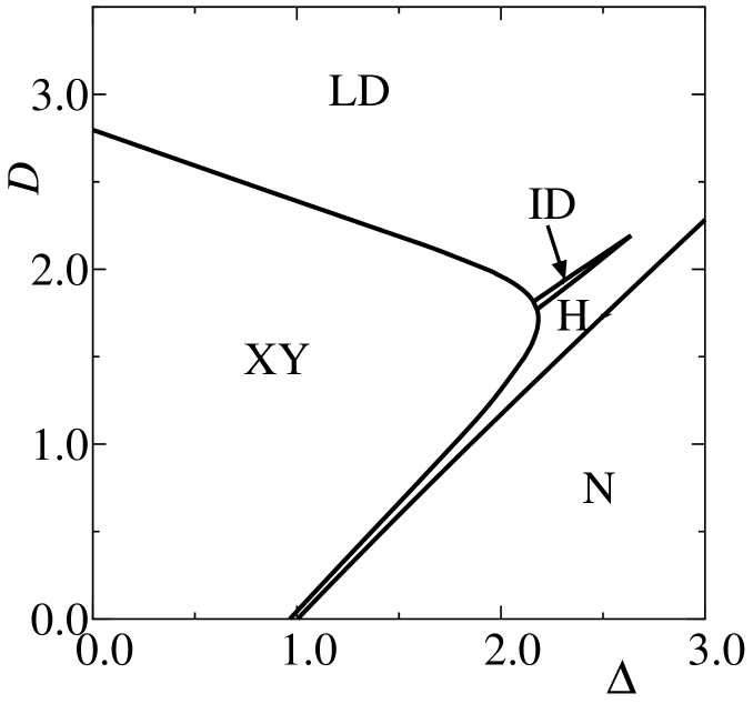
Figure 10: Phase diagram of an $S=2$ chain. H and N are the abbreviations of Haldane and Néel, respectively.

Figure 11: Enlarged phase diagram near the ID phase.

Our final phase diagram is shown in Figs. 11 and 11. The remarkable natures of the phase diagram are: (1) there exists the ID phase which was predicted by Oshikawa in 1992 and has been believed to be absent for a long time; (2) the Haldane state and the LD state belong to the same phase.

We would like to express our appreciation to Professor Masaki Oshikawa and Dr. Frank Pollmann for their invaluable discussions and comments. We also thank the Supercomputer Center, Institute for Solid State Physics, University of Tokyo, the Computer Room, Yukawa Institute for Theoretical Physics, Kyoto University and the Cyberscience Center, Tohoku University for computational facilities. The present work has been supported in part by a Grant-in-Aid for Scientific Research (B) (No. 20340096), and a Grant-in-Aid for Scientific Researches on Priority Areas “Novel states of matter induced by frustration” from the Ministry of Education, Culture, Sports, Science and Technology.

References

References

- [1] Tonegawa T, Okamoto K, Nakano H, Sakai T, Nomura K and Kaburagi M 2011 J. Phys. Soc. Jpn 80 No.4
- [2] Schulz H J 1986 Phys. Rev. B 34 6372
- [3] Oshikawa M 1992 J. Phys.: Cond. Matter 4 7469
- [4] Schollwöck U and Jolicœur Th 1995 Europhys. Lett. 30 493
- [5] Schollwöck U, Golinelli O and Jolicœur Th 1996 Phys. Rev. B 54 4038
- [6] Aschauer H and Schollwöck U 1998 Phys. Rev. B 58 359
- [7] Nomura K and Kitazawa A 1998 J. Phys. A: Math. Gen. 31 7341
- [8] Kitazawa A 1997 J. Phys. A: Math. Gen. 30 L285
- [9] Pollmann F, Berg E, Turner A M and Oshikawa M 2009 arXiv:0909.4059