A new renormalization group approach for systems with strong electron correlation

Abstract

The anomalous low energy behaviour observed in metals with strong electron correlation, such as in the heavy fermion materials, is believed to arise from the scattering of the itinerant electrons with low energy spin fluctuations. In systems with magnetic impurities this scattering leads to the Kondo effect and a low energy renormalized energy scale, the Kondo temperature $T_{\rm K}$. It has been generally assumed that these low energy scales can only be accessed by a non-perturbative approach due to the strength of the local inter-electron interactions. Here we show that it is possible to circumvent this difficulty by first suppressing the spin fluctuations with a large magnetic field. As a first step field-dependent renormalized parameters are calculated using standard perturbation theory. A renormalized perturbation theory is then used to calculate the renormalized parameters for a reduced magnetic field strength. The process can be repeated and the flow of the renormalized parameters continued to zero magnetic field. We illustrate the viability of this approach for the single impurity Anderson model. The results for the renormalized parameters, which flow as a function of magnetic field, can be checked with those from numerical renormalization group and Bethe ansatz calculations.

I Introduction

Materials which have been classified as having strong electron correlation are those which have itinerant electrons in narrow bands arising from atomic d and f states. The effective on-site inter-electron interaction for electrons in these shells is of the order, or greater than, the band widths so that the direct application of perturbation theory to models of these systems, such as the Hubbard model or periodic Anderson model, is not valid in most parameter regimes — particularly in the regimes where anomalous behaviour is expected. The same applies for impurity models, such as the Anderson impurity model, where the anomalous low energy scale, the Kondo temperature $T_{\rm K}$, occurs only when the impurity electron is almost localised and experiences a strong on-site interaction. For this reason the search has been for non-perturbative techniques that can handle the strong on-site interactions. Such non-perturbative techniques as the numerical renormalization group (NRG) Wil75 ; KWW80a and Bethe ansatz (BA) AFL83 ; TW83 have had considerable success in tackling most impurity problems, and some significant progress has been made in understanding the behaviour of lattice models, such as the Mott-Hubbard metal-insulator transition, using dynamical mean field theory (DMFT) GKKR96 in conjunction with a non-perturbative impurity solver. Many other aspects of strong correlation behaviour, such as quantum criticality and the competition between various low temperature broken symmetry states, both magnetic and superconducting, are still very much open problems where there is a need for new ideas and techniques. A feature of strongly correlated systems is that there are low lying electronic collective excitations, which scatter strongly the itinerant electrons. In systems with a strong on-site interaction $U(>0)$, these are usually spin excitations, arising from the effective ferromagnetic or antiferromagnetic exchange interactions, which appear explicitly in models such as the t-J models, which can be derived from a Hubbard model when $U$ is large, where the antiferromagnetic exchange term $J\sim t^{2}/U$ and $t$ is the hopping matrix element.

Here we put to the test a new approach for accessing the low energy scales by applying it to an impurity Anderson model in the strong correlation regime. We have accurate results for this model from the Bethe ansatz (BA) and the numerical renormalisation group (NRG) which we can use to check our results. The motivation is to develop a technique which we can apply to a wider class of models. The Bethe ansatz, though powerful, is restricted to integrable models, which cover a wide class of impurity models, and some one dimensional models such as the Hubbard model, but there is no generalisation to models of higher dimension. The NRG can only be applied to impurity models which have a low degeneracy of impurity states so that the matrix sizes do not become too large for practical iterative diagonalisation. In conjunction with the DMFT the NRG can also be applied to infinite dimensional models which can be mapped into effective impurity models. The density matrix renormalisation group (DMRG) PWKH98 is an alternative form which has been applied successfully to one dimensional systems. There are also functional forms of the renormalisation group (fRG) KBS10 and non-perturbative RG approaches which are at present being developed and applied with some success, but the problem of dealing with the strong correlation of models for systems in two and three dimensions is still an open challenge.

The approach we consider here is based on a renormalised perturbation theory (RPT). The RPT has been developed and tested in detail for the Anderson impurity model Hew93 ; Hew01 . We begin by giving a brief description of this application and then consider the problems in applying the method more generally, and how they might be overcome.

The Hamiltonian for the Anderson model And61 is

$$H_{\rm AM}=\sum_{\sigma}\epsilon_{\mathrm{d},\sigma}d^{\dagger}_{\sigma}d_{\sigma}+Un_{\mathrm{d},\uparrow}n_{\mathrm{d},\downarrow}$$ (1)

$$+\sum_{{k},\sigma}(V_{k,\sigma}d^{\dagger}_{\sigma}c_{{k},\sigma}+V_{k,\sigma}^{*}c^{\dagger}_{{k},\sigma}d_{\sigma})+\sum_{{k},\sigma}\epsilon_{{k},\sigma}c^{\dagger}_{{k},\sigma}c_{{k},\sigma},$$

where $\epsilon_{\mathrm{d},\sigma}=\epsilon_{\rm d}-\sigma g\mu_{\rm B}H/2$ is the energy of the localised level at an impurity site in a magnetic field $H$, $U$ the interaction at this local site, and $V_{k,\sigma}$ the hybridization matrix element to a band of conduction electrons of spin $\sigma$ with energy $\epsilon_{k,\sigma}=\epsilon_{k}-\sigma g_{c}\mu_{\rm B}H/2$, where $g_{c}$ is the g-factor for the conduction electrons. When $U=0$ the local level broadens into a resonance, corresponding to a localised quasi-bound state, whose width depends on the quantity $\Delta_{\sigma}(\omega)=\pi\sum_{k}|V_{k,\sigma}|^{2}\delta(\omega-\epsilon_{k,\sigma})$. For the impurity model, where we are interested in universal features, it is usual to take a wide conduction band with a flat density of states so that $\Delta_{\sigma}(\omega)$ becomes independent of $\omega$, and can be taken as a constant $\Delta_{\sigma}$. In this wide band limit $\Delta_{\sigma}(\omega)$ will be independent of the magnetic field on the conduction electrons, so we can effectively put $g_{c}=0$. When this is the case $\Delta_{\sigma}$ is usually taken to be a constant $\Delta$ independent of $\sigma$. We also introduce the notation $h=g\mu_{\rm B}H/2$.

In the renormalized perturbation theory approachHew93 ; Hew01 we cast the corresponding Lagrangian for this model ${\cal L}_{\rm AM}(\epsilon_{\mathrm{d},\sigma},\Delta,U)$ into the form,

$${\cal L}_{\rm AM}(\epsilon_{\mathrm{d},\sigma},\Delta,U)={\cal L}_{\rm AM}(\tilde{\epsilon}_{\mathrm{d},\sigma},\tilde{\Delta}_{\sigma},\tilde{U})+{\cal L}_{\rm ct}(\lambda_{1,\sigma},\lambda_{2,\sigma},\lambda_{3}),$$ (2)

where the renormalized parameters, $\tilde{\epsilon}_{\mathrm{d},\sigma}$ and $\tilde{\Delta}_{\sigma}$, are defined in terms of the self-energy $\Sigma_{\sigma}(\omega,h)$ of the one-electron Green’s function for the impurity state,

$$G_{\sigma}(\omega,h)={1\over\omega-\epsilon_{\mathrm{d}\sigma}+i\Delta-\Sigma_{\sigma}(\omega,h)},$$ (3)

and are given by

$$\tilde{\epsilon}_{\mathrm{d},{\sigma}}=z_{\sigma}(\epsilon_{\mathrm{d},{\sigma}}+\Sigma_{\sigma}(0,h)),\quad\tilde{\Delta}_{\sigma}=z_{\sigma}\Delta,$$ (4)

where $z_{\sigma}$ is given by $z_{\sigma}={1/{(1-\Sigma_{\sigma}^{\prime}(0,h))}}$. The renormalized or quasiparticle interaction $\tilde{U}(h)$, is defined in terms of the local total 4-vertex $\Gamma^{(4)}_{\uparrow\downarrow}(\omega_{1},\omega_{2},\omega_{3},\omega_{4};h)$ at zero frequency,

$$\tilde{U}(h)=z_{\uparrow}z_{\downarrow}\Gamma^{(4)}_{\uparrow\downarrow}(0,0,0,0;h).$$ (5)

It will be convenient to rewrite the spin dependent quasiparticle energies in the form, $\tilde{\epsilon}_{{\rm d},\sigma}=\tilde{\epsilon}_{\rm d}(h)-\sigma h\tilde{\eta}(h)$, where

$$\tilde{\epsilon}_{\mathrm{d}}(h)={1\over 2}\sum_{\sigma}\tilde{\epsilon}_{\mathrm{d},{\sigma}},\quad\tilde{\eta}(h)={1\over 2h}\sum_{\sigma}\sigma\tilde{\epsilon}_{\mathrm{d},{\sigma}},$$ (6)

where $\tilde{\epsilon}_{\rm d}(h)$ and $\tilde{\eta}(h)$ are both even functions of the magnetic field $h$.

In terms of the renormalised parameters, the Green’s function takes the form,

$$G_{\sigma}(\omega,h)={z_{\sigma}(h)\over\omega-\tilde{\epsilon}_{\mathrm{d}}(h)+\sigma\tilde{h}+i\tilde{\Delta}_{\sigma}(h)-\tilde{\Sigma}_{\sigma}(\omega,h)},$$ (7)

where $\tilde{h}=\tilde{\eta}(h)h$, and $\tilde{\Sigma}_{\sigma}(\omega,h)$ is the renormalised self-energy given by

$$\tilde{\Sigma}_{\sigma}(\omega,h)=z_{\sigma}(\Sigma_{\sigma}(\omega,h)-\Sigma_{\sigma}(0,h)-\omega\Sigma^{\prime}_{\sigma}(0,h)).$$ (8)

The propagator in the RPT is the free quasiparticle Green’s function,

$$\tilde{G}_{\sigma}(\omega,h)={1\over\omega-\tilde{\epsilon}_{\mathrm{d}}(h)+\sigma\tilde{h}+i\tilde{\Delta}_{\sigma}(h)}.$$ (9)

The expansion is carried out in powers of the interaction $\tilde{U}(h)$ for the complete Lagrangian defined in equation (2). The counter term part of the Lagrangian ${\cal L}_{\rm ct}(\lambda_{1,\sigma},\lambda_{2,\sigma},\lambda_{3})$, given by

$${\cal L}_{\rm ct}(\lambda_{1,\sigma},\lambda_{2,\sigma},\lambda_{3})=$$ (10)

$$\sum_{\sigma}\bar{d}_{\sigma}(\tau)(\lambda_{2,\sigma}\omega+\lambda_{1,\sigma})d_{\sigma}(\tau)+\lambda_{3}n_{d,\uparrow}(\tau)n_{d,\downarrow}(\tau),$$

where $\bar{d}_{\sigma}(\tau)d_{\sigma}(\tau)=n_{d,\sigma}(\tau)$, and $\bar{d}_{\sigma}(\tau)$ and $d_{\sigma}(\tau)$ are the Grassmann fields corresponding to the impurity creation and annihilation operators, which are integrated over in the calculation of the partition function. This part of the Lagrangian essentially takes care of any overcounting. The parameters, $\tilde{\epsilon}_{\mathrm{d},{\sigma}}$, $\tilde{\Delta}_{\sigma}$ and $\tilde{U}$, have been taken to be the fully renormalized ones, and the counter term parameters, $\lambda_{1,\sigma}$, $\lambda_{2,\sigma}$ and $\lambda_{3}$, are required to cancel any further renormalisation. This leads to the renormalisation or over-counting conditions,

$$\tilde{\Sigma}_{\sigma}(0,h)=0,\quad{\partial\tilde{\Sigma}_{\sigma}(\omega,h)\over\partial\omega}\Big{|}_{\omega=0}=0,$$ (11)

and

$$\tilde{\Gamma}_{\uparrow,\downarrow}(0,0,0,0;h)=\tilde{U}(h).$$ (12)

The counter terms are completely determined by these conditions.

Exact results for the Fermi liquid regime, which were first derived in a phenomenological approach by Nozières Noz74 , can be derived from the RPT, working only to second order in $\tilde{U}$. We give some of these results for the particle-hole symmetric model. In this case, $\tilde{\epsilon}_{d}(h)=0$ and $\tilde{\Delta}_{\sigma}$ is independent of $\sigma$, so we drop the $\sigma$ index for this quantity. The free quasiparticle density of states $\tilde{\rho}_{\sigma}(\omega,h)$, given by the spectral density of the free quasiparticle Green’s function in equation (9), takes the form,

$$\tilde{\rho}_{\sigma}(\omega,h)=\rho^{(0)}_{\sigma}(\omega,\tilde{h},\tilde{\Delta}(h)),$$ (13)

where $\rho^{(0)}_{\sigma}(\omega,h,\Delta)$ is the local density of states for the non-interacting system,

$$\rho^{(0)}_{\sigma}(\omega,h,\Delta)={1\over\pi}{\Delta\over(\omega+\sigma h)^{2}+\Delta^{2}}.$$ (14)

As $\rho^{(0)}_{\sigma}(\omega,h,\Delta)$ becomes independent of $\sigma$ for $\omega=0$, we can drop the $\sigma$ index when $\omega=0$.

The impurity contribution to the coefficient of the electronic specific heat $\gamma(h)$ is directly proportional to the quasiparticle density of states,

$$\gamma(h)={2\pi^{2}k^{2}_{\rm B}\over 3}\tilde{\rho}(0,h),$$ (15)

where $k_{\rm B}$ is the Boltzmann constant. The induced magnetisation $M(h)$ is given by $M(h)=g\mu_{\rm B}m(h)$, where

$$m(h)={1\over 2}(\langle n_{{\rm d}\uparrow}\rangle-\langle n_{{\rm d}\downarrow}\rangle)=m_{0}(\tilde{h},\tilde{\Delta}(h)),$$ (16)

where $\langle n_{{\rm d}\sigma}\rangle$ is the expectation value of the occupation number of the impurity site, $n_{{\rm d}\sigma}$, and $m_{0}(h,\Delta)$ is the magnetisation for the non-interacting model given by

$$m_{0}(h,\Delta)={1\over\pi}\,{\rm tan}^{-1}\left({h\over\Delta}\right).$$ (17)

The longitudinal susceptibility $\chi_{l}(h)$ (in units of $(g\mu_{\rm B})^{2}$) is given by

$$\chi_{l}(h)={\tilde{\rho}(0,h)(1+\tilde{U}(h)\tilde{\rho}(0,h))/2},$$ (18)

and the local charge susceptibility $\chi_{c}(h)$ is given by

$$\chi_{c}(h)=2{\tilde{\rho}(0,h)(1-\tilde{U}(h)\tilde{\rho}(0,h))}.$$ (19)

The perpendicular susceptibility $\chi_{\perp}(h)$ is given by

$$\chi_{\perp}(h)=\frac{m(h)}{2h},$$ (20)

in the limit of zero transverse field Hew06 .

Asymptotically exact results can also be derived for low energy dynamic spin and charge susceptibilities by taking into account repeated quasiparticle scattering Hew06 . The longitudinal dynamic spin susceptibility is given by

$$\chi_{l}(\omega,h)={\Pi_{l}(\omega,\tilde{h},\tilde{\Delta}(h))\over 2(1-\tilde{U}_{s}(h)\Pi_{l}(\omega,\tilde{h},\tilde{\Delta}(h)))},$$ (21)

for the symmetric model, where

$$\Pi_{l}(\omega,h,\Delta)={\Delta\over{\pi(h^{2}+\Delta^{2})}}\quad{\rm for}\quad\omega=0,$$

$$={-\Delta\over{\pi\omega(\omega+2i\Delta)}}\left\{{\rm ln}\left({{\omega+i\Delta-h}\over{i\Delta-h}}\right)+{\rm ln}\left({{\omega+i\Delta+h}\over{i\Delta+h}}\right)\right\},$$ (22)

for $\omega\neq 0$, where $\tilde{U}_{s}(h)$ is the effective quasiparticle interaction in the longitudinal channel given by $\tilde{U}_{s}(h)=\tilde{U}(h)/(1+\tilde{U}(h)\tilde{\rho}(0,h))$.

The corresponding expression for the transverse susceptibility $\chi^{+-}(\omega,h)$ which we denote by $\chi_{t}(\omega,h)$ is

$$\chi_{t}(\omega,h)={\Pi_{t}(\omega,\tilde{h},\tilde{\Delta}(h))\over 1-\tilde{U}_{t}(h)\Pi_{t}(\omega,\tilde{h},\tilde{\Delta}(h))}.$$ (23)

where

$$\Pi_{t}(\omega,h,\Delta)={i\over{\pi(i\Delta-h)}}-{1\over 2\pi\Delta}{\rm ln}\left({{i\Delta-h}\over{i\Delta+h}}\right)\quad\omega=-2h,$$

$$={-i\over\pi}\left\{{1\over\omega+2h+2i\Delta}{\rm ln}\left({\omega+i\Delta+h\over i\Delta+h}\right)\right.-$$

$$\quad\quad{1\over\omega+2h}\left.{\rm ln}\left({\omega+i\Delta+h\over i\Delta-h}\right)\right\}\quad\omega\neq-2h.$$ (24)

The effective quasiparticle interaction in this channel $\tilde{U}_{t}(h)$ is determined by the condition that the dynamic transverse susceptibility at $\omega=0$ it is equal to twice the static perpendicular susceptibility given in equation (20), $\chi_{t}(0,h)=2\chi_{\perp}(h)$. This gives

$$\chi_{t}(0,h)={{m_{0}(\tilde{h},\tilde{\Delta})\over\tilde{h}}\over 1-{\tilde{U}_{t}(h)m_{0}(\tilde{h},\tilde{\Delta})\over\tilde{h}}}={m_{0}(\tilde{h},\tilde{\Delta})\over h},$$ (25)

on using the result $\Pi_{t}(0,h,\Delta)=m_{0}(h,\Delta)/h$ for $\omega=0$. We then find $\tilde{U}_{t}(h)$ must be such that

$$\tilde{h}=h+\tilde{U}_{t}(h)m(h).$$ (26)

With $\tilde{U}_{t}(h)$ defined as in equation (25), the exact expression for the magnetisation takes the form of a mean field equation,

$$m(h)={1\over\pi}{\rm tan}^{-1}\left({h+\tilde{U}_{t}(h)m(h)\over\tilde{\Delta}(h)}\right).$$ (27)

The only equations that we have quoted that are not exact are the equations for the dynamic susceptibilities $\chi_{l}(\omega,h)$ and $\chi_{t}(\omega,h)$ for finite frequency $\omega\neq 0$. They have nevertheless been shown to provide a very good approximation to the NRG results for these quantities over the whole low frequency range and satisfy the Korringa-Shiba relation exactly (for more details see reference Hew06 ).

To evaluate these formulae we need to know the renormalised parameters. In the Kondo regime, in the absence of a magnetic field, these can be reduced to a single parameter Hew93 , the Kondo temperature $T_{\rm K}$ ($\chi_{l}(0)=1/4T_{\rm K}$) such that

$$\tilde{U}(0)=\pi\tilde{\Delta}(0)=4T_{\rm K},$$ (28)

but this parameter is still undetermined. The most accurate way of calculating the parameters in terms of the ’bare’ parameters of the model, $\epsilon_{d}$, $\Delta$ and $U$, is an indirect one, from an analysis of the low energy fixed point in an NRG calculation. The procedure for doing this is described elsewhere HOM04 . This approach works very well but restricts the method to models where we can apply the NRG, which means one where we already have a solution. It is, nevertheless, a useful adjunct to the NRG, enabling one to calculate many quantities more easily and more accurately. However, we want to develop a way of calculating the renormalised parameters which is independent of the NRG and can be applied more widely. The obvious method would be to calculate them directly from their definitions in equations (4) and (5), but this would again seem to require having a solution, at least for the low energy behaviour of the self-energy. A direct perturbation approach to calculate the self-energy would not seem to offer the possibility of accessing the strong correlation regime, as we know for the symmetric model, low order perturbation theory is unreliable for $U/\pi\Delta>1$, and no-one has so far succeeded in summing a subclass of terms to give the correct low energy behaviour.

We do know, however, that for this model the large renormalisation effects arise for large positive $U$ from the scattering of local low energy spin fluctuations. If we apply a strong local magnetic field these spin fluctuations are suppressed, so the renormalisation effects are much weaker, and perturbation theory can be applied in this case, even in the regime $U/\pi\Delta\gg 1$ HZ84 . This implies that in the limit of a very large magnetic field, we can evaluate the renormalised parameters directly from equations (4) and (5), using perturbation results for the self-energy. This assumption can be checked, as we have results for the Anderson model of the renormalised parameters for any value of the magnetic field, deduced using the NRG Hew05 ; HBK06 ; BH07a . An example is shown in figure 1 for the symmetric Anderson model, with a value of $U/\pi\Delta=3$, $\pi\Delta=0.1$, such that in very low magnetic fields we are in the strong correlation regime with a Kondo temperature $T_{\rm K}=0.002$. The degree of renormalisation in zero field can be estimated from $1/z=\Delta/\tilde{\Delta}$, corresponding to a mass enhancement factor, which in this case gives $1/z\sim 12.7$.

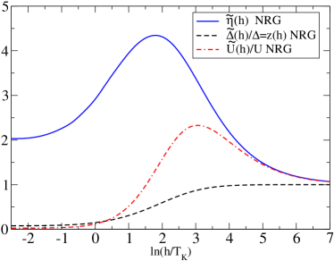
Figure 1: Plots of the renormalised parameters, $\tilde{\Delta}(h)/\Delta$, $\tilde{U}(h)/U$ and $\tilde{\eta}(h)$, for the symmetric Anderson model, calculated using the NRG for the case $\pi\Delta=0.1$, $U/\pi\Delta=3$ as a function of the logarithm of the magnetic field $h/T_{\rm K}$, where $T_{\rm K}=\pi\tilde{\Delta}(0)/4=0.002$.

We can see from figure 1 that $z$ increases monotonically with increase in the value of the magnetic field. It does, however, need extremely large field values, such that $h\sim U$, before the renormalisation effects are completely suppressed. The other two parameters, $\tilde{\eta}(h)$ and $\tilde{U}(h)$, do not simply increase monotonically as the magnetic field is increased. Initially they increase rather slowly, and then rise much more rapidly to a peak value, and then in the extreme large field limit approach their bare values. The initial increase is not surprising because the spin fluctuations are being suppressed and the quasiparticles are becoming less renormalised, the first stage of their undressing. We see that the peak value of $\tilde{U}(h)$ is greater than the bare value $U$. This is because at this point we are approaching the regime where mean field theory and RPA are applicable. In this regime, RPA corresponds to substituting $\tilde{U}_{s}(h)\to U$ and $\tilde{U}_{t}(h)\to U$, with $\tilde{\Delta}(h)\to\Delta$ into equations (21) and (23), giving $\tilde{h}\to\bar{h}=h+Um(h)$ and from equation (18), $\tilde{U}(h)\to U/(1-U\rho^{(0)}(0,\bar{h},\Delta))$. This can explain why $\tilde{U}(h)$ can be enhanced over the bare value $U$. As $\rho^{(0)}(0,\bar{h},\Delta)\to 0$ as $h\to\infty$, the enhancement disappears for very large field values. The other term contributing to $\tilde{U}(h)$ from the $z$-factor in (5) has the opposite effect. In the mean field regime for very large fields, where $z(h)=1$, it has no effect but plays a dominant role in reducing $\tilde{U}(h)$ in the weak field regime where $z(h)$ is small.

The peak in $\tilde{\eta}(h)$ can be explained in a similar way. For large fields we have the mean field result for $\tilde{\eta}(h)=1+Um(h)/h$, so that $\tilde{\eta}(h)\to 1$ as $h\to\infty$ because $m(h)\to 1/2$. It follows from equations (16) and (18) that in the limit $h\to 0$ the value of $\tilde{\eta}(0)$ is equal to the Wilson $\chi/\gamma$ ratio, which in the strongly correlated (Kondo) regime takes the value 2. The fact the $z(h)$ increases as $h^{2}$ for small $h$ explains the initial increase of $\tilde{\eta}(h)$ with $h$. That a peak should occur at an intermediate field value follows as the likely behaviour from the extrapolated trends at low and large field values.

We have conjectured that we should be able to explain the NRG results for the renormalised parameters in the large magnetic field limit using the leading perturbational corrections arising from mean field theory and RPA. The question then arises: Can we find a way to continue the process to lower magnetic fields, as the renormalised parameters in large fields are continuously connected to the strongly renormalised values in the weak field regime? We know that if we start at the other limit, with the zero field renormalised parameters known, we can use the RPT to calculate the renormalised self-energy in a weak field $h$ Hew01 . From this result, we could then calculate the change in the renormalised parameters due to the introduction of the weak magnetic field. We could generalise this idea by considering that we know the parameters for an arbitrary magnetic field value $h$, and use these to calculate the self-energy for a system with a slightly smaller or larger magnetic field $h\pm\delta h$, and hence deduce the renormalised parameters for these neighbouring magnetic field values. This would give a set of scaling equations for the renormalised parameters as a function of the magnetic field. If we can obtain good starting values from perturbation theory in the large field limit, we should be able to reduce iteratively the magnetic field, and scale into the strongly correlated weak field regime. The aim of this paper is to test the feasibility of this scheme, and we use the results from the NRG and Bethe ansatz to test any approximation. We begin first of all looking at the behaviour in the limit of large magnetic field.

II Large magnetic field limit

A formally exact expression can be written down for the self-energy $\Sigma_{\sigma}(\omega)$ in terms of skeleton diagrams, where the propagators correspond to the full many-body Green’s function $G_{d,\sigma}(\omega)$, as given in equation (3), and the full vertex $\Gamma^{(4)}_{\sigma,-\sigma}(\omega_{1},\omega_{2},\omega_{3},\omega_{4})$,

$$\Sigma_{\sigma}(\omega)=U\langle n_{d,-\sigma}\rangle+U\int\int G_{d,\sigma}(\omega+\omega^{\prime})G_{d,-\sigma}(\omega^{\prime\prime})$$

$$G_{d,-\sigma}(\omega^{\prime\prime}-\omega^{\prime})\Gamma^{(4)}_{\sigma,-\sigma}(\omega+\omega^{\prime},\omega^{\prime\prime}-\omega^{\prime},\omega^{\prime\prime},\omega){d\omega^{\prime}\over 2\pi i}{d\omega^{\prime\prime}\over 2\pi i}$$ (29)

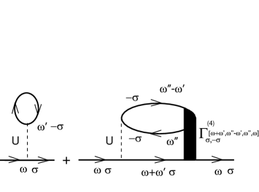
Figure 2: The skeleton diagrams for the self-energy $\Sigma_{\sigma}(\omega)$ in terms of the 4-vertex $\Gamma_{\sigma,-\sigma}^{(4)}$

A diagrammatic representation of this equation is given in figure 2. The skeleton diagrammatic formulation of the perturbation theory is particularly useful when self-consistent approximations are used. The simplest self-consistent approach is the mean field theory where only the tadpole diagram, corresponding to the first term in equation (29), is taken into account. For the particle-hole symmetric model this gives $\Sigma_{\sigma}(\omega)=-\sigma Um(h)$, where $m(h)$ is determined self-consistently from the equation,

$$m(h)={1\over\pi}\,{\rm tan}^{-1}\left({\bar{h}\over\Delta}\right),$$ (30)

where $\bar{h}=h+Um(h)$. Note that we have not included the constant term $U/2$ in the self-energy because for the symmetric model it can always be absorbed into the energy level $\epsilon_{d}$ ($=-U/2$) to give $\epsilon_{d}=0$. From equation (26) this implies that in the mean field regime $\tilde{U}_{t}(h)\to U$. For this approximation we deduce the renormalised parameters, $\tilde{\eta}(h)$ and $\tilde{\Delta}(h)$. As the self-energy is independent of $\omega$, it follows that $z(h)=1$, so

$$\tilde{\eta}(h)=1+{U\over\pi h}\,{\rm tan}^{-1}\left({\bar{h}\over\Delta}\right),\quad\tilde{\Delta}(h)=\Delta,$$ (31)

where $m(h)$ is determined self-consistently from (30). We can deduce the static longitudinal susceptibility by differentiating $m(h)$ with respect to $h$, and from equation (18) deduce $\tilde{U}$. The result is $\tilde{U}_{s}(h)=U$, or equivalently,

$$\tilde{U}(h)={U\over 1-U\rho^{(0)}(0,\bar{h},\Delta)}.$$ (32)

We anticipated this result in the previous section, based on the RPA approximation for the longitudinal dynamical susceptibility.

We now have a 1-1 correspondence between the RPT results and the mean field/RPA equations in the transverse spin scattering channel, and we conjecture that asymptotically for very large magnetic field values,

$$\tilde{h}\to\bar{h}=h+Um(h),\quad\tilde{\Delta}(h)\to\Delta,\quad\tilde{U}_{t}(h)\to U.$$ (33)

In figure 3 we compare the mean field results for $z(h)=\tilde{\Delta}(h)/\Delta$, $\tilde{U}_{t}(h)/U$ and $\tilde{\eta}(h)$, with the corresponding results calculated using the NRG as a function of ${\rm ln}(h/T_{\rm K})$, for the model for $\pi\Delta=0.1$ and $U/\pi\Delta=3$. As expected the mean field results are in agreement with the NRG results for asymptotically large magnetic fields. The mean field results give a good approximation for these parameters for values of $h>90T_{\rm K}$ (${\rm ln}(h/T_{\rm K})>4.5)$. Though the mean field results are only valid for very large magnetic field values, we can build upon them by expanding about the mean field solution. The propagators in the perturbation expansion now take into account the mean field self-energy so that the tadpole diagrams, or mean field insertions, no longer appear explicitly.

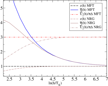
Figure 3: A comparison of the renormalised parameters, $\tilde{\eta}(h)$ $z(h)=\tilde{\Delta}(h)/\Delta$ and $\tilde{U}_{t}(h)/U$, from mean field theory with those calculated using the NRG, for the symmetric Anderson model, with $\pi\Delta=0.1$, $U/\pi\Delta=3$ as a function of the logarithm of the magnetic field $h/T_{\rm K}$, where $T_{\rm K}=\pi\tilde{\Delta}(0)/4$.

For $U>\pi\Delta$ in the absence of a magnetic field, the mean field solution predicts a state with a local magnetic moment, such that it costs no energy to flip the local moment. This is reflected in the dynamic transverse spin susceptibility, calculated with mean field propagators, which develops a singularity at $\omega=0$. Hence, the most important corrections to the self-energy are likely to arise from these spin flip scattering processes. In evaluating the self-energy using equation (29) we need to include the dominant spin flip scattering terms contributing to the 4-vertex $\Gamma^{(4)}_{\sigma,-\sigma}(\omega+\omega^{\prime},\omega^{\prime\prime}-\omega^{\prime},\omega^{\prime\prime},\omega)$, which are illustrated in figure 4. These diagrams are the same as those which are taken into account in the RPA expression for the transverse dynamic susceptibility $\chi_{t}(\omega)$. Summing this class of diagrams gives as an approximation for the 4-vertex, $\Gamma^{(4)}_{\uparrow,\downarrow}(\omega+\omega^{\prime},\omega^{\prime\prime}-\omega^{\prime},\omega^{\prime\prime},\omega)$,

$${U\over 1-U\Pi_{t}(\omega^{\prime},\bar{h},\Delta)}$$ (34)

Substituting this result into equation (29) gives the result,

$$\Sigma_{\uparrow}(\omega,h)=U^{2}\int G^{\rm mf}_{\downarrow}(\omega+\omega^{\prime},\bar{h})\chi_{t}(\omega^{\prime},h){d\omega^{\prime}\over 2\pi i},$$ (35)

where the Green’s function $G^{\rm mf}_{\downarrow}(\omega,\bar{h})$ is the mean field propagator and the transverse dynamic susceptibility $\chi_{t}(\omega,h)$ is calculated in the RPA. There is a similar expression for the spin down self-energy, but with particle-hole symmetry they can be reduced to a single equation as $G_{\downarrow}(\omega,h)=-G_{\uparrow}(-\omega,h)$.

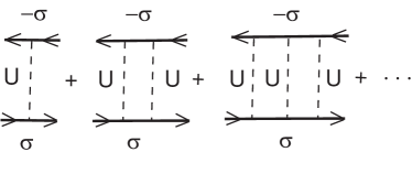
Figure 4: The RPA diagrams that contribute to the 4-vertex $\Gamma^{(4)}_{\sigma,-\sigma}(\omega+\omega^{\prime},\omega^{\prime\prime}-\omega^{\prime},\omega^{\prime\prime},\omega)$

As the self-energy acquires a dependence on the frequency $\omega$ in this approximation, in the calculation of the renormalised parameters, there will be a change of the quasiparticle weight factor $z(h)$ from the mean field value 1. We can see from the results for the renormalised parameters calculated using this result, shown in figure 5, that this leads to a significant improvement in comparing the results with those calculated using the NRG. The renormalised parameters are plotted as a function of ${\rm ln}(h/T_{\rm K})$ for the same parameter set as in figure 3, $\pi\Delta=0.1$, $U/\pi\Delta=3$. The values for both $z(h)$ and $\tilde{U}_{t}(h)$ are now seen to decrease with a decrease in $h$ in a rather similar way to the NRG results. The value of $\tilde{\eta}(h)$ also develops a peak as the magnetic field value is reduced in a similar way to the NRG results, but the calculations for this quantity break down for ${\rm ln}(h/T_{\rm K})<-0.5$. The results now constitute a good approximation to the NRG results down to a magnetic value $h\sim 27T_{\rm K}$ corresponding to ${\rm ln}(h/T_{\rm K})\sim 3.4$.

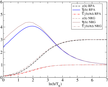
Figure 5: A comparison of the renormalised parameters, $\tilde{\eta}(h)$ $z(h)=\tilde{\Delta}(h)/\Delta$ and $\tilde{U}_{t}(h)/U$, using the RPA propagator in calculating the self-energy with those calculated using the NRG, for the symmetric Anderson model, with $\pi\Delta=0.1$, $U/\pi\Delta=3$ as a function of the logarithm of the magnetic field $h/T_{\rm K}$, where $T_{\rm K}=\pi\tilde{\Delta}(0)/4$.

We have derived, using perturbation theory, asymptotically exact expressions for the renormalised parameters for very large magnetic field values. However, the magnetic field regime where these results are valid is completely outside the range that can be realised experimentally, except possibly for some quantum dot systems. We need a way of extending the calculations to much lower magnetic field values. It should be possible, in principle at least, to improve on these results by systematically taking corrections to the RPA into account. However, this gets more and more difficult, involving multiple frequency integrations and more complex self-consistent equations to solve. Our aim here is a limited one, the calculation of the renormalised parameters which depend only on the form of the self-energy in the low frequency regime, and as a result we can adopt a different strategy for carrying out higher order calculations. We return to the idea discussed at the end of the Introduction, that we might be able to use the RPT, with renormalised parameters for a magnetic field $h$, to calculate the renormalised self-energy at a reduced fields value $h-\delta h$, and hence derive the renormalised parameters for the lower magnetic field value $h-\delta h$.

III Calculations using the RPT

The RPT approach differs from standard perturbation theory as it includes counter terms. We should consider how to handle these terms, and test various approximations for calculating the renormalised self-energy $\tilde{\Sigma}_{\sigma}(\omega,h)$ in a given magnetic field $h$, using the renormalised parameters, $\tilde{\eta}(h)$, $\tilde{\Delta}(h)$ and $\tilde{U}(h)$, for the same magnetic field value $h$, before considering how to use them for a system with a reduced magnetic field.

When RPT calculations are carried out to a specific order $n$ in powers of $\tilde{U}$, we can handle the counter terms by also expanding them formally in powers of $\tilde{U}$, and taking into account all diagrams generated to order $n$, including those involving the counter terms. Counter term contributions of order greater then $n$ will not contribute and the terms up to order $n$ can be determined, order by order, by requiring them to satisfy the renormalisation conditions given in equations (11) and (12) (see reference Hew01 for a specific example). We need a more general procedure, however, for calculations based on summing subclasses of diagrams taken to infinite order.

There are five counter terms to deal with, four of them, $\lambda_{1,\sigma}$ and $\lambda_{2,\sigma}$ involve one-body terms, and the fifth is an interaction term $\lambda_{3}$. The contributions arising from the diagrams for the counter terms, $\lambda_{1,\sigma}$ and $\lambda_{2,\sigma}$, alone, can be taken into account fully as they do not involve the interaction term. The interaction counter term $\lambda_{3}$ can be added to the interaction $\tilde{U}$, and the expansion carried out in powers of the total interaction term $\tilde{U}+\lambda_{3}$. The value of $\lambda_{3}$ is then required to satisfy the renormalisation condition in equation (12). The local Green’s function subject to a magnetic field $h$, using the renormalised parameters for the field $h$, takes the form,

$$G_{\sigma}(\omega,h)=$$ (36)

$${z(h)\over\omega+\sigma\tilde{h}+i\tilde{\Delta}(h)+\lambda_{1,\sigma}+\omega\lambda_{2,\sigma}-\tilde{\Sigma}^{S}_{\sigma}(\omega,h)}.$$

where $\tilde{\Sigma}^{S}_{\sigma}(\omega,h)$ is the self-energy calculated using the quasiparticle propagator, $\tilde{G}_{\sigma}(\omega,h)=G_{\sigma}(\omega,h)/z(h)$, which includes the two counter terms, $\lambda_{1,\sigma}$ and $\lambda_{2,\sigma}$. This means that the self-energy $\tilde{\Sigma}^{S}_{\sigma}(\omega,h)$ will be a function of $\lambda_{1,\sigma}$ and $\lambda_{2\sigma}$, as well as $\lambda_{3}$, so that the renormalisation conditions in equations (11) take the form,

$$\tilde{\Sigma}^{S}_{\sigma}(0,h,\lambda_{1,\sigma^{\prime}},\lambda_{2,\sigma^{\prime}},\lambda_{3})=\lambda_{1,\sigma},$$ (37)

and

$${\partial\tilde{\Sigma}^{S}_{\sigma}(\omega,h,\lambda_{1,\sigma^{\prime}},\lambda_{2,\sigma^{\prime}},\lambda_{3})\over\partial\omega}\Big{|}_{\omega=0}=\lambda_{2,\sigma}.$$ (38)

Given a result for $\tilde{\Sigma}^{S}_{\sigma}(0,h)$, calculated from a particular subset of diagrams, the conditions in equations (37) and (38) generate self-consistent equations which must be solved to determine the counter terms, $\lambda_{1,\sigma}$ and $\lambda_{2,\sigma}$.

We can now perform calculations equivalent to mean field and the RPA but in the RPT framework. At the first mean field stage we only take the tadpole diagrams into account giving $\Sigma^{S}_{\sigma}(\omega,h)=-\sigma(\tilde{U}+\lambda_{3})m(h)$. In this approximation from equations (37) and (38) we get $\lambda_{1,\sigma}=\sigma(\tilde{U}+\lambda_{3})m(h)$ and $\lambda_{2,\sigma}=0$, so

$$G^{\rm mf}_{\sigma}(\omega,h)={1\over\omega+\sigma\tilde{h}+i\tilde{\Delta}(h)}.$$ (39)

The next stage is to calculate the transverse susceptibility $\chi_{t}(\omega,h)$, using propagators which include the mean field insertions. The $\lambda_{1,\sigma}$ in the propagator given in equation (57) cancels the mean field term, the propagator now becomes the free propagator given in equation (9). The result for $\chi_{t}(\omega,h)$ is

$$\chi_{t}(\omega,h)={\Pi_{t}(\omega,\tilde{h},\tilde{\Delta}(h))\over 1-(\tilde{U}+\lambda_{3})\Pi_{t}(\omega,\tilde{h},\tilde{\Delta}(h))}.$$ (40)

The counter term $\lambda_{3}$ has yet to be determined. We have the exact result, $\chi_{t}(0,h)=m(h)/h$, which from (40) implies $\tilde{h}+(\tilde{U}+\lambda_{3})m(h)$, so we can identify $\tilde{U}+\lambda_{3}$ as $\tilde{U}_{t}(h)$ in equation (26) and the expression for $\chi_{t}(\omega,h)$ with that given in equation (23). The interaction term $\tilde{U}_{t}(h)$ expressed in terms of the two other renormalised parameters, $\tilde{\Delta}(h)$ and $\tilde{\eta}(h)$, is

$$\tilde{U}_{t}(h)={h(\tilde{\eta}(h)-1)\over m(h)}={\pi h(\tilde{\eta}(h)-1)\over{\rm tan}^{-1}(h(\tilde{\eta}(h)/\tilde{\Delta}(h))}.$$ (41)

Detailed comparison of the RPT results for the transverse susceptibility based equations (40) (or equivalently (23)) and (41) with a direct NRG calculations have been given earlier Hew06 . They are in remarkably good agreement with the NRG results for all values of the magnetic field over a magnetic field range $-10T_{\rm K}<h<10T_{\rm K}$, asymptotically exact as $\omega\to 0$, and satisfy the Korringa-Shiba relation.

We can derive an approximation for the self-energy $\tilde{\Sigma}^{S}_{\uparrow}(\omega,h)$ analogous to that given in equation (35),

$$\tilde{\Sigma}^{S}_{\uparrow}(\omega,h)=\tilde{U}_{t}^{2}(h)\int\tilde{G}^{\rm mf}_{\downarrow}(\omega+\omega^{\prime},h)\chi_{t}(\omega^{\prime},h){d\omega^{\prime}\over 2\pi i}.$$ (42)

Some RPT results based on equations (42) and (40) for the self-energy and one-electron spectral density have also been given earlier Bau07 ; BHO07 and compared with the corresponding results from direct NRG calculation. Again the agreement between the two sets of results was very good over a low frequency range $-0.5T_{\rm K}<\omega<0.5T_{\rm K}$ for $h=0$ and over a larger range for higher values of $h$. These results demonstrate that it is possible to find an approximation using the RPT which will accurately reproduce the form of the self-energy in the low frequency regime for any value of the magnetic field.

IV RPT calculations in the low field limit

We need to extend the RPT calculations described in the previous section to see if, given with renormalised parameters for one field value, we can calculate the self-energy for another field value, and hence deduce how the renormalised parameters change as we vary the magnetic field. Before we consider this problem in detail we consider the simpler case of using the renormalised parameters for $h=0$ to calculate the renormalised self-energy in the presence of a weak magnetic field $h$. As we want to keep the magnetic field term explicitly in the Hamiltonian, and as the self-energy has the form $\Sigma_{\sigma}(\omega+\sigma h,h)$, we modify our procedure and use a slightly different form for the remainder term $\Sigma^{\rm rem}_{\sigma}(\omega+\sigma h,h)$ via

$$\Sigma_{\sigma}(\omega+\sigma h,h)=\Sigma_{\sigma}(0,0)+$$ (43)

$$(\omega+\sigma h){\partial\Sigma_{\sigma}(\omega+\sigma h,h)\over\partial\omega}\Big{|}_{\omega=h=0}+\Sigma^{\rm rem}_{\sigma}(\omega+\sigma h,h).$$

As the renormalised parameters are those defined for $h=0$, the renormalised self-energy and 4-vertex satisfies the equations in (11) and (12) with $h$ set equal to zero. Substituting this form into the equation (3) for the impurity Green’s functions gives

$$G_{\sigma}(\omega,h)={z\over\omega-\tilde{\epsilon}_{\mathrm{d}}+\sigma h+i\tilde{\Delta}-\tilde{\Sigma}^{r}_{\sigma}(\omega,h)},$$ (44)

so the renormalised parameters now correspond to $h=0$, and the renormalised self-energy is defined by

$$\tilde{\Sigma}^{r}(\omega,h) =z\Big{\{}\Sigma_{\sigma}(\omega+\sigma h,h)-\Sigma_{\sigma}(0,0)-$$ (45)

$$(\omega+\sigma h){\partial\Sigma_{\sigma}(\omega+\sigma h,h)\over\partial\omega}\Big{|}_{\omega=h=0}\Big{\}}.$$

Note that this self-energy for $h\neq 0$ is different from the self-energy $\tilde{\Sigma}(\omega,h)$ defined earlier in equation (8), due to the different remainder term, so we use a slightly different notation to distinguish them. The renormalised self-energy $\tilde{\Sigma}^{r}(\omega,h)$ is required to satisfy the equation in (11) for $h=0$.

We now show that exact result for $\tilde{\Sigma}^{r}(0,h)$ to first order in $h$ is given by the self-consistent evaluation of the tadpole diagram as in mean field theory. The counter term $\lambda_{1}$ only cancels off the tadpole diagram for $h=0$, so taking this into account, we get for the renormalised self-energy, $\tilde{\Sigma}^{r}_{\uparrow}(\omega,h)=-(\tilde{U}+\lambda_{3})m(h)$, with

$$m(h)={1\over\pi}{\rm tan}^{-1}\left({h-\tilde{\Sigma}^{r}_{\uparrow}(0,h)\over\tilde{\Delta}}\right).$$ (46)

This equation for $m(h)$ corresponds to the exact form given by the Friedel sum rule. Solving these mean field equations to first order in $h$, we find for the zero field susceptibility,

$$\chi_{l}={\pi\tilde{\Delta}\over 2(1-(\tilde{U}+\lambda_{3})/\pi\tilde{\Delta})}.$$ (47)

This result for $\chi_{l}$ corresponds to the exact result given in equation (18) if $\tilde{U}+\lambda_{3}=\tilde{U}_{s}$. For $h=0$ we also have $\tilde{U}_{t}=\tilde{U}_{s}$ so this mean field equation corresponds to the exact one given earlier in equation (27), but with the renormalised parameters $\tilde{\Delta}(h)$ and $\tilde{U}_{t}(h)$ taken at zero field. As the corrections to the zero field values for $\tilde{\Delta}(h)$ and $\tilde{U}_{t}(h)$ are of order $h^{2}$, it follows that equation (27) with the zero field renormalised parameters is exact to first order in $h$.

We can extend the calculations to include an $\omega$-dependence in $\tilde{\Sigma}^{r}_{\sigma}(\omega,h)$ by using the RPT equation (42) with the zero field parameters in the transverse dynamic susceptibility calculated from the NRG. From the change in the linear $\omega$-dependence of the renormalised self-energy with the magnetic field $h$, we can calculate the change $\Delta z(h)=z(h)-z(0)$. We can then compare the results with the corresponding value of $\Delta z(h)$ deduced from a direct NRG calculation of the self-energy. A comparison of the two sets of results is shown in figure 6 for the case $U/\pi\Delta=3$, $\pi\Delta=0.1$. It can be seen that the two sets of results are in complete agreement in the very low field regime. This implies that, given the renormalised parameters at $h=0$, we should be able to calculate accurately both the change in $z(h)$ and the shift in the real part of the self-energy with $h$, provided we use a sufficiently small value of $h$. This is all the information we require to calculate the renormalised parameters for small $h$ from the given values at $h=0$.

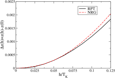
Figure 6: A plot of the change in $z(h)$, $\Delta z(h)=z(h)-z(0)$, as a function of $h/T_{\rm K}$ calculated using the RPT for $U/\pi\Delta=3$, $\pi\Delta=0.1$, with renormalised prameters at $h=0$ deduced from the NRG, compared with $\Delta z(h)$ deduced from a direct NRG calculation of the self-energy.

V Scaling equations

We now consider how to set up a scaling equation to deduce the renormalised parameters for a magnetic field $h-\delta h$, given a renormalised self-energy that has been calculated using the renormalised parameters, $\tilde{\eta}(h)$, $\tilde{\Delta}(h)$ and $\tilde{U}(h)$ for a magnetic field value $h$. We first of all introduce a renormalised self-energy $\tilde{\Sigma}^{r}_{\sigma}(\omega,h,\delta h)$ following the steps from equation (43) to (45) but retain only the $\delta h$ term explicitly in the Green’s function and the remaining part is absorbed to give the renormalised parameters $\tilde{\eta}(h)$ and $\tilde{\Delta}(h)$ as defined earlier,

$$\tilde{\Sigma}^{r}(\omega,h,\delta h) =z(h)\Big{\{}\Sigma_{\sigma}(\omega,h-\delta h)-\Sigma_{\sigma}(0,h)-$$ (48)

$$(\omega-\sigma\delta h){\partial\Sigma_{\sigma}(\omega,h)\over\partial\omega}\Big{|}_{\omega=\delta h=0}\Big{\}}.$$

The self-energy $\tilde{\Sigma}^{r}(\omega,h,\delta h)$ satisfies the renormalisation conditions in (11) for $\delta h=0$. The local Green’s function for the system with a magnetic field $h-\delta h$, using the parameters for the system in a field $h$, takes the form,

$$G_{\sigma}(\omega,h-\delta h)=$$ (49)

$${z(h)\over\omega-\sigma\delta h+\sigma\tilde{h}(h)+i\tilde{\Delta}(h)-\tilde{\Sigma}^{r}_{\sigma}(\omega,h,\delta h)},$$

where $\tilde{h}(h)=h\tilde{\eta}(h)$. However, in terms of the renormalised parameters for the field value $h-\delta h$, this Green’s function is

$$G_{\sigma}(\omega,h-\delta h)=$$ (50)

$${z(h-\delta h)\over\omega+\sigma\tilde{h}(h-\delta h)+i\tilde{\Delta}(h-\delta h)-\tilde{\Sigma}_{\sigma}(\omega,h-\delta h)}.$$

We can find an expression for the renormalised parameters $\tilde{h}(h-\delta h)$ and $z(h-\delta h)$ in terms of the parameters for $\delta h=0$ and the self-energy $\tilde{\Sigma}^{r}_{\sigma}(\omega,h,\delta h)$ by equating the inverses of the Green’s functions in equations (49) and (50). Differentiating these with respect to $\omega$, and putting $\omega=0$, gives

$$z(h-\delta h)=\bar{z}(h,\delta h)z(h),$$ (51)

where $\bar{z}(h,\delta h)=1/(1-\tilde{\Sigma}^{r^{\prime}}_{\sigma}(0,h,\delta h))$. Hence we get a relation between $\tilde{\Delta}(h-\delta h)$ and $\tilde{\Delta}(h)$,

$$\tilde{\Delta}(h-\delta h)=\bar{z}(h,\delta h)\tilde{\Delta}(h).$$ (52)

Equating the inverses of (49) and (50) and putting $\omega=0$, we find a relation between $\tilde{h}(h-\delta h)$ and $\tilde{h}(h)$,

$$\tilde{h}(h-\delta h)=\bar{z}(h,\delta h)(\tilde{h}(h)-\delta h-\tilde{\Sigma}^{r}_{\uparrow}(0,h,\delta h)).$$ (53)

We can find a alternative form of this equation by expanding $\tilde{\Sigma}^{r}_{\uparrow}(0,h,\delta h)$ to first order in $\delta h$ and then using the relation,

$${\partial\tilde{\Sigma}^{r}_{\uparrow}(0,h,\delta h))\over\partial\delta h}\Big{|}_{\delta h=0}=-\tilde{\rho}(0,h)\tilde{U}(h),$$ (54)

which follows from the Ward identity Yam75a ; Yam75b ; Hew01 . We then get an equation for $\tilde{h}(h-\delta h)$ in the form,

$$\tilde{h}(h-\delta h)=\bar{z}(h,\delta h)(\tilde{h}(h)-\delta h(1+R(h)))+{\rm O}[(\delta h)^{2}],$$ (55)

where $R(h)$ is the Wilson ratio given by $R(h)=1+\tilde{\rho}(0,h)\tilde{U}(h)$.

We also need to be able to calculate the new interaction term $\tilde{U}_{t}(h-\delta h)$. It can be seen from equation (41) that a knowledge of $\tilde{\eta}(h)=\tilde{h}(h)/h$ and $\tilde{\Delta}(h)$ is sufficient to determine $\tilde{U}_{t}(h)$. Hence from the results for $\tilde{\Delta}(h-\delta h)$ and $(\tilde{h}-\delta h)$ we can deduce $\tilde{U}_{t}(h-\delta h)$.

Finally, the full renormalised vertex $\tilde{U}(h-\delta h)$ can be calculated from the results for $\tilde{\Delta}(h-\delta h)$ and $\tilde{\eta}(h-\delta h)$, by differentiating the magnetisation, as given in equation (16), to determine the static longitudinal susceptibility, and then equating it to the expression given in equation (18).

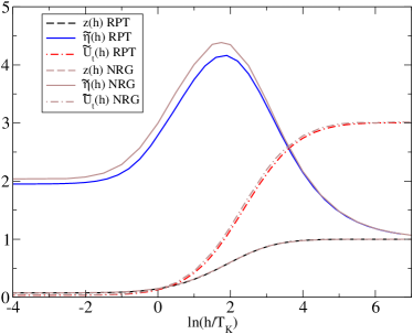
Figure 7: A comparison the renormalised parameters, $z(h)=\tilde{\Delta}(h)/\Delta$, $\tilde{U}_{t}(h)/U$ and $\tilde{\eta}(h)$ as calculated from the RPT and NRG for the symmetric Anderson model, with $\pi\Delta=0.1$, $U/\pi\Delta=3$ as a function of the logarithm of the magnetic field $h/T_{\rm K}$, where $T_{\rm K}=\pi\tilde{\Delta}(0)/4$.

We now have to amend the procedure outlined in the previous section to calculate the self-energy in the reduced field $\tilde{\Sigma}^{r}_{\uparrow}(\omega,h,\delta h)$ so that we can exploit equations (52) and (53) or (55) to extend the calculation of the renormalised parameters to smaller values of the field.

VI Extension to lower magnetic field values

The Green’s function for a system with a magnetic field $h-\delta h$, in terms of renormalised parameters for a field value $h$, takes a form similar to that given in equation (36) when we include the counter terms $\lambda_{1,\sigma}(h)$ and $\lambda_{2,\sigma}(h)$,

$$G_{\sigma}(\omega,h-\delta h)=$$ (56)

$${z(h)\over\omega+\sigma(\tilde{h}-\delta h)+i\tilde{\Delta}(h)+\lambda_{1,\sigma}+\omega\lambda_{2,\sigma}-\bar{\Sigma}^{r}_{\sigma}(\omega,h,\delta h)}.$$

The self-energy $\bar{\Sigma}^{r}_{\sigma}(\omega,h,\delta h)$ is now calculated with the quasiparticle propagator,

$$G_{\sigma}(\omega,h-\delta h)=$$ (57)

$${1\over\omega+\sigma(\tilde{h}-\delta h)+i\tilde{\Delta}(h)+\lambda_{1,\sigma}+\omega\lambda_{2,\sigma}-\bar{\Sigma}^{r}_{\sigma}(\omega,h,\delta h)}.$$

The counter terms $\lambda_{1,\sigma}$ and $\lambda_{2,\sigma}$, however, are still determined by the conditions given in equations (37) and (38) but with $\delta h=0$.

We consider first of all the tadpole diagram, which now gives a finite contribution because it is not cancelled completely by the counter term for $\delta h\neq 0$. This diagram, when the cancellation due to the counter term $\lambda_{1,\sigma}$ has been taken into account gives $\tilde{\Sigma}^{r}_{\sigma}(\omega,h,\delta h)=-\sigma\tilde{U}_{t}(h)m(h,\delta h)$ where

$$m(h,\delta h)={1\over\pi}{\rm tan}^{-1}\left({-\delta h-\tilde{\Sigma}^{r}_{\uparrow}(0,h,\delta h)\over\tilde{\Delta}}\right).$$ (58)

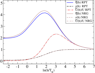
Figure 8: A comparison of the renormalised parameters, $\tilde{\Delta}(h)/\Delta$, $\tilde{U}(h)/U$ and $\tilde{\eta}(h)$ calculated using the RPT as a function of the logarithm of the magnetic field $h/T_{\rm K}$, compared with the corresponding results from the NRG given in figure 1.

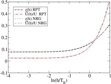
Figure 9: The NRG and RPT results for $\tilde{\Delta}(h)/\Delta$ and $\tilde{U}(h)/U$ as in figure 7 over the the low field regime.

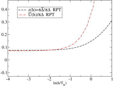
Figure 10: The renormalised parameters, $z(h)=\tilde{\Delta}(h)/\Delta$, $\tilde{U}(h)/\pi\Delta$ as calculated from the RPT for the same parameter set as in figure 1, showing to a good approximation the approach to the zero field strong coupling result $\tilde{U}=\pi\tilde{\Delta}$.

The mean field self-consistent equation for $m(h,\delta h)$ is then solved, and this term absorbed into the propagator in equation (57) so the perturbation expansion is now about this mean field solution. The next step is to take the repeated quasiparticle scattering term into account in the calculation of the self-energy $\tilde{\Sigma}^{r}_{\sigma}(\omega,h,\delta h)$ as in equation (42). This constitutes our approximation for calculating $\tilde{\Sigma}^{r}_{\sigma}(\omega,h,\delta h)$. The renormalised parameters as a function of magnetic field can now be calculated for a field $h-\delta h$ using this approximation for $\tilde{\Sigma}^{r}_{\sigma}(\omega,h,\delta h)$ together with the scaling equations (52) and (53) or (55).

In figure 7 we compare the results for $\tilde{\eta}(h)$, $\tilde{U}_{t}(h)$ and $z(h)=\tilde{\Delta}(h)/\Delta$ obtained in the RPT, using the scaling equation to extend to the low field regime, with the NRG results. The results are for the symmetric model with $U/\pi\Delta=3$, $\pi\Delta=0.1$. It can be seen that the agreement with the NRG results is very good over the whole magnetic field range, especially the results for $\tilde{U}_{t}(h)$ and $z(h)=\tilde{\Delta}(h)/\Delta$. The results for $\tilde{\eta}(h)$ are smaller than the NRG results at lower field values but the difference is relatively small. In the very low field regime $h\to 0$, the NRG results approach the value 2 corresponding to the Wilson ratio in the Kondo limit. The RPT results in this regime are smaller by approximately 3%.

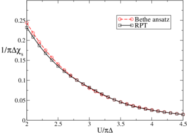
Figure 11: A comparison of $1/\pi\Delta\chi_{s}$ for $h=0$ as deduced from the RPT (full curve) with the Bethe ansatz results (dashed curve) for a range of values of $U/\pi\Delta$. In the strong correlation regime $1/\pi\Delta\chi_{s}\to 4T_{\rm K}/\pi\Delta$.

Within the approximation we have used we can calculate $\tilde{U}(h)$, given $\tilde{U}_{t}(h)$ and $\tilde{\eta}(h)$, rather more simply than the method described earlier, by summing the renormalised equivalent of the diagrams in figure 4 to give

$$\tilde{U}(h)={\tilde{U}_{t}(h)\over 1-\tilde{U}_{t}(h)\Pi_{t}(0,\tilde{h},\tilde{\Delta}(h))}.$$ (59)

Using the fact that $\Pi_{t}(0,\tilde{h},\tilde{\Delta}(h))=m_{0}(\tilde{h},\tilde{\Delta}(h))/\tilde{h}$, we find $\tilde{U}(h)=\tilde{h}\tilde{U}_{t}(h)/h=\tilde{\eta}(h)\tilde{U}_{t}(h)$.

In figure 8 we compare the results for $\tilde{\eta}(h)$, $\tilde{U}(h)$ and $z(h)=\tilde{\Delta}(h)/\Delta$ obtained in the RPT using the scaling with the NRG results as given in figure 1 for the same parameter set. There is excellent agreement between the $\tilde{U}(h)$ from the RPT with the NRG result. As the values of $z(h)=\tilde{\Delta}(h)/\Delta$ and $\tilde{U}(h)$ are rather small in the strong coupling regime $h\to 0$, we give an enlarged picture of the comparison of the results in the weak field regime in figure 9. The agreement of the RPT with the NRG results can be seen to be maintained down to values of the magnetic field several orders of magnitude less than the Kondo temperature $T_{\rm K}$. Finally in figure 10 we give a plot of the RPT values of $\tilde{U}(h)/\pi\Delta$ and $\tilde{\Delta}(h)/\Delta$. The fact that the two curves merge as $h\to 0$ shows that the RPT results asymptotically satisfy the relation $\tilde{U}(0)=\pi\tilde{\Delta}(0)$, as given in equation (28) corresponding to a single renormalised energy scale.

In figure 11 we compare the results for $1/\pi\Delta\chi_{s}$ from the RPT calculation in the zero field limit for a range of values of $U/\pi\Delta$ with the corresponding Bethe ansatz results HZ85 given by

$${1\over\pi\Delta\chi_{s}}={4T_{\rm K}\over(1+I)\pi\Delta},$$ (60)

where

$${T_{\rm K}}=\left({U\Delta\over 2}\right)^{1/2}e^{-\pi U/8\Delta+\pi\Delta/2U},$$ (61)

and

$$I={1\over\sqrt{\pi}}\int_{0}^{\pi\Delta/2U}{e^{x-\pi^{2}/16x}\over\sqrt{x}}\,dx.$$ (62)

For $U/\pi\Delta>2$, the integral term $I$ is very small compared to unity so that in this regime ${1/\pi\Delta\chi_{s}}$ corresponds to ${4T_{\rm K}/\pi\Delta}$.

It can be seen from this comparison there is very good agreement with the Bethe ansatz results in the strong correlation regime $U/\pi\Delta>2.5$. It shows clearly that the RPT results give the correct form for $T_{\rm K}$ in the Kondo regime, not only in the exponential dependence on $U$ but also in the prefactor. There is a progressive improvement in the agreement with the exact Bethe ansatz results with increase of $U/\pi\Delta$ over the range $2\leq U/\pi\Delta\leq 4.5$.

It might seem surprising to be able to get such precise agreement by taking what would appear to be only a subclass of diagrams into account. The explanation is that we are considering the low energy regime and, for strong correlation, the dominant low energy scattering is with the spin fluctuations. The low energy charge fluctuations are suppressed in this regime and their effects can be taken into account by suitably renormalised vertices. For smaller values of $U/\pi\Delta$ the charge fluctuations begin to play a role and have to be considered explicitly. In this regime they cannot be taken into account simply by the use of an effective frequency independent vertices.

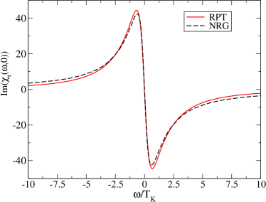
Figure 12: A plot of ${\rm Im}\chi_{t}(\omega,0)$ versus $\omega/T_{\rm K}$ for $U/\pi\Delta=3$, $\pi\Delta=0.1$ and $h=0$, as calculated directly from the NRG (dashed curve) and from the RPT with renormalised parameters also calculated using the RPT.

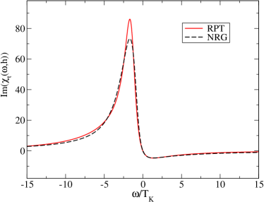
Figure 13: A plot of ${\rm Im}\chi_{t}(\omega,h)$ versus $\omega/T_{\rm K}$ for $U/\pi\Delta=3$, $\pi\Delta=0.1$ and $h=T_{\rm K}=0.002$, as calculated directly from the NRG (dashed curve) and from the RPT with renormalised parameters also calculated using the RPT.

We are now in a position to calculate the low energy dynamic susceptibility and self-energy at $h=0$ and low fields entirely from the RPT. In figures 12 and 13 we compare the RPT results for the imaginary part of the dynamic transverse susceptibility (full curve) with the corresponding results calculated directly from the NRG (dashed curve) for the case $U/\pi\Delta=3$ and $\pi\Delta=0.1$ and $h=0$ and $h=T_{\rm K}$ respectively. These have been calculated using equation (23) for $\chi_{t}(\omega,h)$ with the renormalised parameters. It can be seen that they are in good agreement over the whole low frequency regime. The discrepancy in the peak height in figure 13 is almost certainly due to the logarithmic broadening used in the NRG calculations which has the effect of reducing the height of any peak displaced from the origin. The higher the magnetic field value the larger the effect becomes as the peak gets shifted further from the origin Hew06 .

In figures 14 and 15 we make a similar comparison of the RPT results for the imaginary part of the self-energy calculated to second order in $\tilde{U}$ for the same set of parameters, $U/\pi\Delta=3$ and $\pi\Delta=0.1$ and $h=0$ and $h=T_{\rm K}$. The imaginary part of the self-energy $\Sigma_{\sigma}(\omega,h)$ is related to the imaginary part of the renormalised self-energy $\tilde{\Sigma}_{\sigma}(\omega,h)$ from equation (8) via

$${\rm Im}\Sigma_{\sigma}(\omega,h)={1\over z(h)}\,{\rm Im}\tilde{\Sigma}_{\sigma}(\omega,h).$$ (63)

There is very good agreement between the two sets of curves over the range $|\omega|\leq 0.5T_{\rm K}$. The small discrepancy in the low frequency regime in figure 15 could be due to the imaginary part of the self-energy in the NRG results does not precisely equal zero at $\omega=0$. Surprisingly, using the RPT only to second order in $\tilde{U}$ for $h=0$ extends the range of the agreement to $|\omega|\leq T_{\rm K}$.

The low order RPT calculations give the asymptotically exact results corresponding to Fermi liquid theory in the low frequency regime. However, once the renormalised parameters have been calculated the renormalised perturbation theory is completely defined, and can be extended to higher frequency and higher energy scales by taking higher order diagrams into account. The extension to the higher frequency range is currently being studied, and some preliminary results have been published Hew01 ; BHO07 .

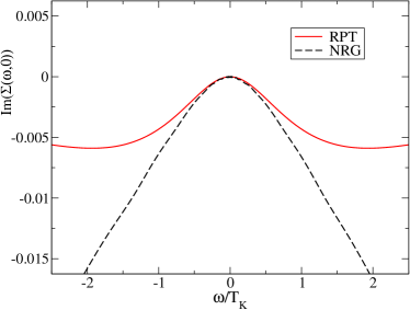
Figure 14: A plot of the imaginary part of the self-energy $\Sigma_{\uparrow}(\omega,0)$ versus $\omega/T_{\rm K}$ for $U/\pi\Delta=3$, $\pi\Delta=0.1$ and $h=0$, as calculated directly from the NRG (dashed curve) and from the RPT with renormalised parameters also calculated using the RPT.

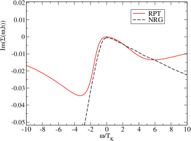
Figure 15: A plot of the imaginary part of the self-energy $\Sigma_{\uparrow}(\omega,h)$ versus $\omega/T_{\rm K}$ for $U/\pi\Delta=3$, $\pi\Delta=0.1$ and $h=T_{\rm K}$, as calculated directly from the NRG (dashed curve) and from the RPT with renormalised parameters also calculated using the RPT.

VII Conclusions

We have set out to see whether we can access the low energy behaviour of a strongly correlated system using a renormalised form of perturbation theory which would be applicable to a general class of models. We have taken as a test case the particle-hole symmetric single impurity Anderson model with parameters in the strongly correlated Kondo regime, where we have exact results which can be used to test any approximation used. The approach has been based on the renormalised perturbation theory, which has previously been shown to give asymptotically exact results for this model in the low energy regime in terms of renormalised parameters. Hitherto these renormalised parameters have been calculated in terms of the bare parameters that specify the model from an analysis of the low energy fixed point of an NRG calculation. The renormalised parameters can be determined very accurately using this indirect approach, but this makes the method dependent on the NRG. Our goal has been to find an alternative and more general way to calculate these parameters, and to test the approximations used by comparing the results with those derived using the NRG. To do this we have exploited the fact that the low energy spin fluctuations, which cause the strong renormalisation effects, can be suppressed by the application of a very strong magnetic field, allowing standard perturbation theory to be applied and the renormalised parameters to be calculated in the large field regime. The renormalised perturbation theory is then used to calculate the renormalised parameters on reducing the field $h$ by a small amount to $h-\delta h$, so setting up a scaling relation. The solution of this scaling equation allows the field value to be extended down to $h=0$. The approximation used has been based on a mean field-like theory at each stage with a self-energy that includes the RPA-like fluctuations about the mean field. The results for the renormalised parameters have been compared with those calculated in previous work using the NRG for the complete magnetic field range. This relatively simple approximation scheme gives remarkably good results for magnetic field values down to $h=0$, as demonstrated in the comparison with the Bethe ansatz results for the zero temperature susceptibility. This calculation demonstrates that it is possible to access the strong correlation regime using a perturbational analysis.

There are some similarities with the approach used here for the Anderson model with two other perturbational approaches. In the local moment approach LET98 ; LD01b RPA diagrams are included in a two self-energy formalism, where the self-energies are constructed from a mean field broken symmetry state for $h=0$. The symmetry, which should be restored by the low energy dynamics, is then imposed by the requirement that the imaginary part of self-energy is zero at $\omega=0$, which determines the mean field magnetisation. This approach has an advantage in giving an interpolation such that the high energy features, corresponding to the atomic states, are included, and does give a low energy scale $T_{\rm K}$ which depends exponentially on $U/\pi\Delta$ with an exponent in agreement with the Bethe ansatz result TW83 . The fact that the symmetry has to be imposed, however, rather than develop naturally as the field is reduced in the RPT approach, is a limitation.

The other related approaches have been based on the functional renormalisation group. A recent example is the work of Bartosch et al. BFRK09 who use a Hubbard-Stratonovich transformation and include both longitudinal and transverse spin fluctuations in calculating the self-energy. A cut off $\Lambda$ was imposed to suppress the low energy spin fluctuations, which plays a role similar to the large applied field used in the RPT. Flow equations for the renormalised vertices as a function of $\Lambda$ were then derived based using various approximations based on the truncation of the higher order vertices. The results, however, for the quasiparticle weight factor $z$, which should behave as $z\sim T_{\rm K}/\Delta$ in the Kondo regime, did not have the exponential dependence on $U/\pi\Delta$.

The demonstration of the feasibility of this RPT approach has been for a specific model, for a particular parameter set. The method, however, is a rather general one, and should be applicable to more general impurity models. A good test case would be the general $n$-channel Anderson model with a Hund’s rule exchange term. The renormalised parameters have been calculated for this model using the NRG for $n=2$ NCH10 , but for $n>2$ the NRG calculations become prohibitively difficult due to the sizes of the matrices to be diagonalised. It should also be possible to apply the approach to lattice models of strongly correlated systems, where in an appropriate applied field the low energy behaviour of the system evolves continuously on reducing an appropriate applied field to zero. The next step is to test the approach for these more general types of models.

Acknowledgment

We thank Johannes Bauer, Akira Oguri, Yunori Nishikawa and Daniel Crow for helpful discussions, and EH acknowledges the support of an EPSRC grant.

References

- (1) K. Wilson, Rev. Mod. Phys. 47, 773 (1975).
- (2) H. R. Krishna-murthy, J. W. Wilkins, and K. G. Wilson, Phys. Rev. B 21, 1003 (1980).
- (3) N. Andrei, K. Furuya, and J. H. Lowenstein, Rev. Mod. Phys. 55, 331 (1983).
- (4) A. M. Tsvelik and P. B. Wiegmann, Adv. Phys. 32, 453 (1983).
- (5) A. Georges, G. Kotliar, W. Krauth, and M. J. Rozenberg, Rev. Mod. Phys. 68, 13 (1996).
- (6) I. Peschel, X. Wang, M. Kaulke, and K. Hallberg, Density Matrix Renormalization (Springer, Berlin, 1998).
- (7) P. Kopietz, L. Bartosch, and F. Schütz, Introduction to the Functional Renormalization Group (Springer, Berlin, 2010).
- (8) A. C. Hewson, Phys. Rev. Lett. 70, 4007 (1993).
- (9) A. C. Hewson, J. Phys.: Cond. Mat. 13, 10011 (2001).
- (10) P. W. Anderson, Phys. Rev. 124, 41 (1961).
- (11) P. Nozières, J. Low. Temp. Phys. 17, 31 (1974).
- (12) A. C. Hewson, J. Phys.: Cond. Mat. 18, 1815 (2006).
- (13) A. C. Hewson, A. Oguri, and D. Meyer, Eur. Phys. J. B 40, 177 (2004).
- (14) B. Horvatić and V. Zlatić, Phys. Rev. B 30, 6717 (1984).
- (15) A. C. Hewson, J. Phys. Soc. Japan 74, 8 (2005).
- (16) A. C. Hewson, J. Bauer, and W. Koller, Phys. Rev. B 73, 045117 (2006).
- (17) J. Bauer and A. C. Hewson, Phys. Rev. B 76, 035119 (2007).
- (18) J. Bauer, Renormalisation group study of broken symmetry states in strongly correlated electron systems, PhD thesis, Imperial College London, 2007.
- (19) J. Bauer, A. C. Hewson, and A. Oguri, J. Magn. Magn. Mat. 310, 1133 (2007).
- (20) K. Yamada, Prog. Theo. Phys. 53, 970 (1975).
- (21) K. Yamada, Prog. Theo. Phys. 54, 316 (1975).
- (22) B. Horvatić and V. Zlatić, J. Physique 46, 1459 (1985).
- (23) D. Logan, M. Eastwood, and M. Tusch, J. Phys.: Cond. Mat. 10, 2673 (1998).
- (24) D. Logan and N. Dickens, Europhys. Lett. 54, 227 (2001).
- (25) L. Bartosch, H. Freire, J. R. Cardenas, and P. Kopietz, J. Phys.: Cond. Mat. 21, 305602 (2009).
- (26) Y. Nishikawa, D. J. G. Crow, and A. C. Hewson, Phys. Rev. B 82, 115123 (2010).