Fluctuations and asymmetric jet events
in Pb Pb collisions at the LHC

Abstract

Recent LHC results concerning full jet-quenching in Pb Pb collisions have been presented in terms of a jet asymmetry parameter, measuring the imbalance between the transverse momenta of leading and subleading jets. We examine the potential sensitivity of this distribution to fluctuations from the heavy-ion background. Our results suggest that a detailed estimate of the true fluctuations would be of benefit in extracting quantitative information about jet quenching. We also find that the apparent impact of fluctuations on the jet asymmetry distribution can depend significantly on the choice of low-$p_{t}$ threshold used for the simulation of the hard $pp$ events.

In the quest to understand the properties of the medium generated in high-energy heavy-ion collisions, the past decade has seen extensive study of medium-induced modifications to the production of high transverse momentum objects [1]. It has been conclusively established at RHIC that the spectra of high-momentum hadrons are significantly suppressed, by a factor of $R_{AA}\simeq 0.2$ relative to the appropriate rescaling of the $pp$ spectra. This effect is generally attributed to their (or their originating parton’s) interaction with the medium.

Recently, significant attention has been directed to jets. Compared to hadrons, jets are interesting because, at least in $pp$ collisions, there is a closer, and perturbatively quantifiable, connection between a jet’s momentum and that of its originating parton. STAR [2] and PHENIX [3] have presented first (preliminary) measurements of full jets produced in AuAu collisions with transverse momenta in the $20-40\,\text{GeV}$ range and found that jet spectra are also suppressed, though by a potentially more modest factor than for hadrons. Recently, ATLAS [4] has published studies of the correlations between the momenta of the two leading jets, with the striking observation that a significant fraction of events show a strong imbalance between the $p_{t}$’s of the leading jet and the first subleading jet on the opposite side of the event. CMS has shown similar preliminary results in Ref. [5] and first phenomenological interpretations have been given in Ref. [7].

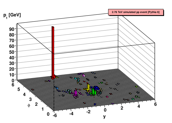
Figure 1: A simulated $pp$ event from Pythia 6.423 (centre-of-mass energy $\sqrt{s}=2.76\,\text{TeV}$; the missing transverse energy was zero). We find that for 1 in every 300 events with a jet with $p_{t1}>100\,\text{GeV}$, the second hardest jet has $p_{t2}<p_{t1}/3$. A more accurate estimation of this number would benefit from the combination of 2-jet, 3-jet, 4-jet, … samples, using for example one of the multijet matching methods reviewed in [8].

Dijet imbalances can occur also in normal $pp$ events, due to emission of multiple gluons (cf. the simulated Pythia event shown in fig. 1), but they are quite rare. To quantify how much more often they arise in Pb Pb collisions, ATLAS and CMS have shown distributions of the jet asymmetry $A_{J}$

$$A_{J}=\frac{E_{T1}-E_{T2}}{E_{T1}+E_{T2}}\,,$$ (1)

expressed in terms of the transverse energies of the leading and subleading jets, respectively $E_{T1}$ and $E_{T2}$. The main quantitative evidence for jet quenching comes in the form of a significant enhancement of the asymmetry in the region around $A_{J}\simeq 0.4$ (fig. 3 of [4] and p. 26 of [5]).

In extracting the distribution of $A_{J}$, the experiments must contend with the fact that each jet may be contaminated with ${\cal O}\left(100-150\,\text{GeV}\right)$ of transverse momentum from the medium particles, usually referred to as the background. To calculate the $A_{J}$ for a given dijet event, each jet’s momentum is corrected for the expected level of background activity in the jet, usually estimated from the activity elsewhere in the event, preferably at similar rapidities (see e.g. [9, 10, 4]). Such a correction cannot, however, account for the fact that the background fluctuates from point to point within the event (even at the same rapidity), so that the momentum subtracted from the jet will inevitably differ from the background actually present in the jet; nor does it account for fluctuations in the detector’s response to the background and jet particles.

Fluctuations are of course a common issue for jet measurements even in $pp$ collisions, notably due to randomness in the response of calorimeters. However two novelties may be relevant concerning fluctuations for heavy-ion collisions. Firstly the LHC heavy-ion medium has only just been produced and it is probably fair to assume that its fluctuations are less well understood than those of the detectors, which have been the object of study for many years. Secondly, the absolute size (i.e. in GeV) of detector fluctuations scales roughly as the square-root of the jet energy, meaning that they are less important for low-$p_{t}$ jets than for high-$p_{t}$ jets, whereas background fluctuations are probably largely independent of the jet’s $p_{t}$.

This last point is relevant because of the way in which fluctuations can affect the $A_{J}$ distribution. The experimental analyses of the $A_{J}$ distribution select events in which the leading jet passes some high-$p_{t}$ cut, say $p_{t}>100\,\text{GeV}$. Events with a genuine high-$p_{t}$ jet are rare. There are many more low-$p_{t}$ dijet events and in some small fraction of cases the background under one of the jets may fluctuate upwards causing the jet to pass the high-$p_{t}$ cut. Such events will naturally have a large jet asymmetry, since there is no reason for the balancing jet to also have a positive background fluctuation. The relative contributions of different classes of events depends on the interplay between the rareness of large background fluctuations and the rareness of high-$p_{t}$ jet production as compared to low-$p_{t}$ jet production. While one can in principle estimate the potential severity of this problem from Monte Carlo simulations, it is debatable whether reliable enough descriptions of the PbPb medium produced at high energy exist. Guidance from experimental measurements is therefore paramount.

One parameter that is indicative of the size of the fluctuations in the reconstructed jet $p_{t}$ is their standard deviation, which we call $\sigma_{\text{jet}}$. ATLAS [11] has presented preliminary results for the fluctuations from one calorimeter tower to the next. If scaled up by the square-root of the number of towers in a jet (about 50 for an $R=0.4$ jet with towers of size $0.1\times 0.1$ in rapidity and azimuth), it would suggest a value $\sigma_{\text{jet}}\simeq 8.5\,\text{GeV}$ for the most central set of events. On the other hand, the scaling of the tower fluctuations by the square-root of the number of towers may not be a safe way of extrapolating tower fluctuations to $\sigma_{\text{jet}}$, insofar as the background could well have local correlations (there is no clear reason for the correlation length of such fluctuations to necessarily be smaller than the calorimeter tower size). Furthermore there can be other factors that contribute to a degradation of resolution, such as back reaction [12] and fluctuations in the event-by-event (or calorimeter-strip) estimation of the background level (as discussed in sections 3.5 and A.1 of [10]).

Another way in which one may attempt to deduce the level of the fluctuations is from a preliminary inclusive jet spectrum for $0-100\%$ centrality (p. 41 of [11]), which displays a region of near Gaussian $p_{t}$-dependence for $p_{t}\lesssim 50$ that is strongly suggestive of an origin due to fluctuations, and compatible with $\sigma_{\text{jet}}\simeq 14\,\text{GeV}$. One would then expect the corresponding $\sigma_{\text{jet}}$ for $0-10\%$ central events to be somewhat larger.

Neither of the above estimates, made in the original version of this article, is ideal. One criticism that has been made is that the tower fluctuations do not include full calibration. As for the inclusive jet spectrum, it mixes a genuine jet spectrum in with the fluctuations. However, subsequently, support for $\sigma_{\text{jet}}$ values $\gtrsim 15\,\text{GeV}$ has appeared in the form of a preliminary measurement of the background fluctuations for charged-track jets from ALICE [13]. It is discussed in detail in Appendix A.2.

To provide simple insight into the impact on the dijet asymmetry from various values of $\sigma_{\text{jet}}$, we have carried out the following “toy” analysis. We generate jet events with Pythia [14] (version 6.423, DW underlying-event tune [15]). To mimic the effect of residual fluctuations following background subtraction, we then add to the $p_{t}$ of each jet a random fluctuation, generated according to a Gaussian distribution with mean $0$ and standard deviation $\sigma_{\text{jet}}$, independently of the jet $p_{t}$ (details are given in appendix A.1). These choices correspond to a perfect estimate of the average background that needs subtracting in each event, with $\sigma_{\text{jet}}$ encoding the combination of all sources of fluctuations, whether intrinsic fluctuations of the background, or fluctuations in the detector’s response to it. We select events in which the leading jet has $p_{t}>100\,\text{GeV}$, the subleading jet has $p_{t}>25\,\text{GeV}$, both have rapidities $|y|<2.8$ and are separated in azimuth by $|\Delta\phi|>\pi/2$ and for these events plot the corresponding distribution of $A_{J}$, similarly to the ATLAS analysis [4].

The filled black points in fig. 2 show our results for four different values of $\sigma_{\text{jet}}$. One sees a clear distortion of the $A_{J}$ distribution as $\sigma_{\text{jet}}$ is increased, reminiscent of the pattern seen by ATLAS and CMS with increasing centrality. One key element of our simulation is that in generating the filled black points we chose a fairly low minimum $p_{t}$ cut, $p_{t}^{\min}=30\,\text{GeV}$, for the underlying Pythia $2\to 2$ scattering, and also verified that further lowering this cut made no difference for our values of $\sigma_{\text{jet}}$. With a larger choice, $p_{t}^{\min}=70\,\text{GeV}$ (shaded region), which would be perfectly adequate for low $\sigma_{\text{jet}}$, one notices that a significant part of the effect of the background fluctuations can be missed for larger $\sigma_{\text{jet}}$. This leads to the obvious implication that the choice of $p_{t}^{\min}$ can play an important role, especially if $\sigma_{\text{jet}}$ happens to be large (or, as we have also found, if there are significant non-Gaussianities in the fluctuations).

Pythia with Gaussian smearing

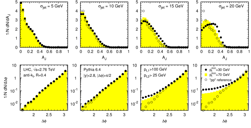
Figure 2: Simulated distribution of $A_{J}$ and $\Delta\phi$, as obtained when smearing the $p_{t}$ of jets from Pythia 6.4 (DW tune [15]) by an amount $\sigma_{\text{jet}}$. None of the results in this figure involved jet quenching. Four different $\sigma_{\text{jet}}$ values are shown, and for each plot there are results from Pythia simulations with two different generation cutoffs on the $2\to 2$ scattering, $p_{t}^{\min}=30\,\text{GeV}$ and $p_{t}^{\min}=70\,\text{GeV}$, so as to illustrate its impact. The results labelled “pp” reference always correspond to $p_{t}^{\min}=30\,\text{GeV}$ with no smearing. Jet clustering has been performed with the anti-$k_{t}$ algorithm [17] with $R=0.4$, as implemented in FastJet [18].

A complementary investigation into the impact of fluctuations can be obtained by embedding Pythia events into a simulated PbPb background. A similar investigation was carried out by ATLAS, embedding events into PbPb events as simulated by an ATLAS-specific version of HIJING [19]. Our analysis will differ in that we study HYDJET [20] rather than HIJING and use also a lower $p_{t}$ cutoff for the Pythia events. The tune we use for HYDJET gives an average background level of $210\,\text{GeV}$ per unit area for $0-10\%$ centrality and $|\eta|<2.8$, compatible with the average jet contamination found by ATLAS, and an average charged-particle multiplicity for $0-10\%$ centrality of 1400 for $|\eta|<0.5$, which is reasonably consistent with that measured by ALICE [21] (further comparisons are discussed in appendix A.2). HYDJET’s simulation of quenching has been turned off, to avoid the potential confusion that might arise from the quenching of hard jets associated with the PbPb simulation rather than with the embedded Pythia event (quenching has only a modest $5-10\%$ effect on the HYDJET fluctuations). Since detectors can have an impact on fluctuations, we have also processed the events through a simplified calorimeter simulation. To subtract the background from jets we have taken the area/median method of [12, 22], using, for the estimation of the background density, a (rapidity) StripRange of half-width 0.8 centred on the jet to be subtracted, as described in more detail in [10]. This method should perform similarly to the ATLAS method of background subtraction. With this setup, for collisions in the 0-10% centrality range, we find fluctuations per unit area of about $23\,\text{GeV}$ corresponding, for anti-$k_{t}$ jets of radius $R=0.4$, to an expected $\sigma_{\rm jet}$ of $16\,\text{GeV}$ and a measured $\sigma_{\rm jet}$ of $17\,\text{GeV}$.

Pythia embedded in HYDJET

Figure 3: Simulated distribution of $A_{J}$ and $\Delta\phi$, as obtained when embedding Pythia events in a PbPb background described by HYDJET 1.6. None of the results in this figure involved jet quenching and the results obtained with HYDJET include a simple calorimeter simulation. Four different centrality regions are shown as indicated in the plots on the top row. For each plot there are results from Pythia simulations with two different generation cutoffs on the $2\to 2$ scattering, $p_{t}^{\min}=10\,\text{GeV}$ and $p_{t}^{\min}=70\,\text{GeV}$, so as to illustrate its impact. The results labelled “pp” reference always correspond to those of Fig. 2. Jet clustering has been performed with the anti-$k_{t}$ algorithm [17] with $R=0.4$, as implemented in FastJet [18] and the heavy-ion background subtraction has been performed as described in [10] with the background density estimated using a StripRange of half-width 0.8 centred on the jet being subtracted.

The results we obtain from the HYDJET+Pythia simulations are presented in Fig. 3 for four centrality ranges. The empty circles labelled “pp” reference correspond to plain Pythia results as for Fig. 2. The filled black points and shaded histogram correspond to our embedding in HYDJET events and differ only by the $p_{t}^{\min}$ of the underlying Pythia $2\to 2$ scattering: $10\,\text{GeV}$ has been used for the former and $70\,\text{GeV}$ for the latter.

The evolution of the $A_{J}$ distribution with increasing centrality in HYDJET displays a pattern similar to that observed for the Gaussian smearing with increasing $\sigma_{\text{jet}}$. If anything, the distortion of the $A_{J}$ distribution for $0-10\%$ central HYDJET collisions is slightly more pronounced at large $A_{J}$ than with the highest Gaussian smearing we used, despite the smaller $\sigma_{\text{jet}}$ value from HYDJET. This could perhaps be a consequence of non-Gaussianities in its fluctuations. The HYDJET results also confirm the importance of the choice of $p_{t}^{\min}$ cut on the $2\to 2$ scatters.

While the above results suggest that fluctuations could be of relevance in interpreting the $A_{J}$ distributions, one should not forget that the experiments have studied observables intended to signal the possible presence of important effects from fluctuations. One such observable is the fraction of energy inside a core of $R=0.2$ within the jet. A fluctuation that enhances the leading jet’s $p_{t}$ would not necessarily be close to the centre of the jet and so should on average reduce the core energy fraction. Preliminary data from ATLAS (p. 34 of [11]) show a stronger reduction in core energy fraction with increasing centrality than in the ATLAS HIJING simulations. In our HYDJET simulations, the core energy fraction decreases yet more rapidly, which at first sight suggests that its fluctuations could be excessive. On the other hand, we find that the agreement in absolute value is better for central collisions than for peripheral collisions, complicating the interpretation. Another cross-check on fluctuations comes from the $A_{J}$ distribution for jets with $R=0.6$ (e.g. p. 48 of [11]). Since fluctuations should increase for a larger $R$, one would expect them to lead to an enhancement of the high $A_{J}$ part of the $R=0.6$ distribution. Vacuum QCD (and jet quenching) are expected to act in the opposite direction. The (unquenched) HYDJET simulation shows a fairly complicated behaviour however: the large $A_{J}$ ($\gtrsim 0.4$) part of the distribution barely changes in going from $R=0.4$ to $R=0.6$, while the distribution increases for $A_{J}=0.2$ (and decreases for $A_{J}$ near zero). In contrast, the preliminary data decrease at large $A_{J}$ and, within the (large) errors, barely change for moderate and small $A_{J}$, suggesting, possibly, some non-trivial interplay between an effect such as quenching and fluctuations.

If fluctuations are relevant, as they seem to be, then it is probably advantageous to attempt to unfold their effect, and/or to reduce their impact by raising the jet $p_{t}$ thresholds. Additionally it may be of interest to investigate methods to suppress fluctuations (the method of [9] as used by CMS [6], or filtering/trimming/pruning [23, 24, 25]). Nevertheless one should be aware that such methods introduce potential biases of their own, as has been found in earlier studies [2, 10], and it then becomes important to quantify the interplay between any quenching and the noise reduction method.

To conclude, we have found that fluctuations can significantly affect the dijet asymmetry $A_{J}$ measured in [4]. A precise estimate of the contribution of fluctuations is therefore important to be able to quantify the degree of quenching that is present in the data. A first direct estimate of these fluctuations has appeared in preliminary form [13] since the original version of our article. It shows fluctuations that are well reproduced by our HYDJET simulations and consistent also, therefore, with the upper end of the range that we explored in the toy model. Quantitative use of the $A_{J}$ data to constrain quenching therefore probably requires that the potential bias due to fluctuations (or from any techniques used to suppress them) be accounted for.

Appendix A Appendix

Since the appearance of the first version of this article, a number of questions have been raised concerning our analysis. Moreover new experimental results have become available. We address these questions here, also in light of the new data.

A.1 Details of our Gaussian smearing procedure

In the discussions that followed the appearance of our article, one question that arose concerned the details of our Gaussian smearing procedure, which we had originally omitted for brevity. The procedure is the following: we generate Pythia events (pp, $\sqrt{s}=2.76\,\text{TeV}$, DW tune); to these we add a low density of “ghost” particles ($10$ per unit area), which have infinitesimal momentum and serve to ensure that there are no substantial empty regions in the event; we then run the anti-$k_{t}$ algorithm with $R=0.4$ on the combination of Pythia and ghost particles. For each jet that is found (however small its momentum, and independently of whether it involves Pythia particles or just ghost-particles) we add to it a random $p_{t}$, chosen according to a Gaussian distribution of zero mean and dispersion $\sigma_{\text{jet}}$. We then consider only the two hardest jets, requiring that they both be above the $25\,\text{GeV}$ threshold.

A criticism was made [26] that only “hard” jets should be fluctuated and that if this choice was made then the deformation of the $A_{J}$ distribution would differ substantially from that seen in fig. 2. The criticism may have its origins in the fact that one of the LHC experiments, CMS, uses a seeded jet algorithm. Depending on the seed threshold, then it might indeed be the case that a hard core is a prerequisite for a jet to be found. For a non-seeded algorithm such as anti-$k_{t}$, fluctuations anywhere in the event may cause a jet to be found, even if there was no corresponding genuine underlying hard jet. This has to be accounted for in the choice of original jets that receive fluctuations. We note that had we not fluctuated zero- and low-$p_{t}$ jets we would not have reproduced the broadening of the low $\Delta\phi$ tail in fig. 2 (which for $\sigma_{\text{jet}}=20\,\text{GeV}$ is comparable to ATLAS’s results for $0-10\%$ centrality).

One criticism that would be legitimate is that some fraction of the anti-$k_{t}$ jets have a very small area and should therefore be subject to smaller fluctuations, whereas we assigned identical fluctuations to all jets. We have examined the impact of a modified version of our procedure, in which the fluctuations scale in proportion to the square-root of the jet area. The results show slightly larger fluctuation-induced asymmetries, perhaps because a modest fraction of anti-$k_{t}$ jets have areas larger than $\pi R^{2}$.

A.2 Fluctuations in ALICE data and HYDJET simulations

To date, the most direct experimental constraint on $\sigma_{\text{jet}}$ comes from an ALICE result presented in a talk [13] a few weeks after the appearance of our note. This involves a measurement of the resolution in the reconstruction of jets from charged tracks only, tested via the embedding of single-track jets. The background subtraction method used there is the area/median method of FastJet. We can directly compare to it by applying our analysis procedure on the charged tracks from HYDJET, with a single additional embedded hard track.

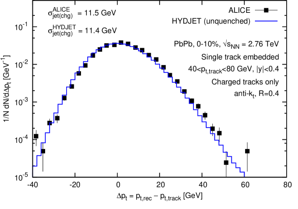
Figure 4: Comparison of our HYDJET simulation to ALICE data [13], showing the distribution of $\Delta p_{t}=p_{t,\text{rec}}-p_{t,\text{track}}$ i.e. the difference in transverse momentum between a reconstructed charged-track jet (anti-$k_{t}$, $R=0.4$) and the single embedded charged track contained within it. $\Delta p_{t}$ is calculated after background subtraction with the Fastjet median/area method. The jets have been reconstructed using charged particles with $|\eta|<0.8$ and $p_{t}>150\,\text{MeV}$, whose masses have been set to zero by rescaling their energy. The background estimation in the HYDJET case used the $k_{t}$ algorithm [27] with $R=0.4$, with particles and ghosts (of area $0.01$) up to $|y|=0.8$ and a global range up to $|y|=0.4$ (excluding the two hardest jets within $|y|<0.8$). We understand that these choices coincide with those made by ALICE.

That comparison is given in fig. 4, which shows the difference between the reconstructed $p_{t}$ of the jet that contains the track and the $p_{t}$ of the track itself. The agreement between the ALICE and HYDJET results is striking, especially considering that our HYDJET simulation had not been directly tuned to LHC data. Quantitatively this can seen by comparing the $\sigma_{\text{jet}(\text{chg})}$ values as obtained from the ALICE data with those from the simulation. We find $\sigma_{\text{jet}\text{(chg)}}\simeq 11.5\,\text{GeV}$ from the ALICE data and $11.4\,\text{GeV}$ in the HYDJET simulation.

Several factors intervene in comparing these results to the $\sigma_{\text{jet}}$ value of $17\,\text{GeV}$ discussed in the main text for full jets embedded in HYDJET. Firstly, in going from the embedding of a single track to that of a full jet, an extra increase of a few percent may arise (e.g. due to back-reaction [10]). More importantly, assuming that a fraction $f_{\text{chg}}\simeq 0.6$ of the energy flow is carried by charged particles, one may expect an additional factor that is somewhere between $\sim 1/\sqrt{f_{\text{chg}}}\simeq 1.3$ (taking charged and neutral components to be uncorrelated) and $\sim 1/f_{\text{chg}}\simeq 1.7$ (for $100\%$ correlated charged and neutral components). Finally there will be additional fluctuations from the calorimetric nature of jet measurements. Combining all these factors gives a result that is consistent with the $\sigma_{\text{jet}}\simeq 17\,\text{GeV}$ quoted in the main text.

Ultimately therefore, the ALICE results support the choices that we made in estimating the possible order of magnitude of fluctuation-induced contributions to the jet-asymmetry measurement. Note however that other issues also need to be taken in to account at the $1-2\,\text{GeV}$ level (for example detector effects). An analysis at this level of accuracy can therefore probably only be performed in conjunction with a fu ll detector simulation.

A.3 Suitability of calorimeter simulation

One objection that has been raised concerning our HYDJET results is that our toy calorimeter simulation suffered from an overly pessimistic resolution. To obtain a detailed description of jet response, ideally many effects need to be taken into account, including tower thresholds, different kinds of noise term that are independence of energy, scale as $1/\sqrt{E}$ and as $1/E$, different responses to photons and charged hadrons, the effect of magnetic fields, and the degradations of resolution due to detector elements that lie between the interaction point and the calorimeter. A full simulation of all these effects goes beyond the scope of this article, therefore we made a simple approximation involving towers of size $0.1\times 0.1$ with a resolution of $0.8/\sqrt{E}$, together with the removal of charged tracks with $p_{t}<0.5\,\text{GeV}$ (on the grounds that they would be bent away from the calorimeter by the magnetic field). The $0.8/\sqrt{E}$ term is larger than the corresponding term for the ATLAS hadronic calorimeter ($\sim 0.5/\sqrt{E}$), however this difference is justified by the fact that we neglect many other sources of detector fluctuation. The validation of this statement is given through fig. 5, which compares the jet resolution that we have observed with our calorimeter (matching calorimeter jets within $\Delta R<0.25$ of the two hardest particle-level jets in an event) to that found by ATLAS. One sees that rather than overestimating calorimeter fluctuations, we actually underestimate them by $5-10\%$ over the full range of $p_{t}$ in which jet resolution measurements exist. Note also that ATLAS has shown that its calorimeter response is similar for jets and heavy-ion backgrounds (p. 37 of [11]).

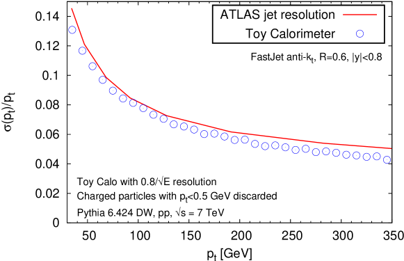
Figure 5: Comparison of jet resolution obtained with our toy calorimeter to the measured ATLAS jet resolution [28].

A further potential issue comes from the fact that an experiment’s magnetic field, by bending particles differently according their $p_{t}$, may smear any angular correlations that are present in the background fluctuations. Our calorimeter simulation did not by default consider the impact of a magnetic field (other than by removing charged particles with $p_{t}<0.5\,\text{GeV}$). We have, however, verified that if one accounts for the effect of a magnetic field on the charged-particles’ azimuth when they reach the calorimeter, the FastJet median/area estimate of fluctuations is reduced by an amount of order $1\%$. This value was obtained with a configuration similar to that used by ATLAS, i.e. a longitudinal magnetic field of strength $B=2$ T, with a calorimeter at a radius of $1.5$ m from the beam. This result gives us confidence that our original approximation was not unreasonable.

If is to be noted that magnetic fields could also have an impact on measurements of quenched jets (independently of background-related issues), insofar as quenching may alter the relative fractions of different momentum components within a jet and therefore also give an appearance of additional jet broadening.

A.4 The CMS jet-reconstruction procedure

It was not the purpose of this article to discuss the CMS results [6], insofar as they appeared subsequent to the first version of this article. However, certain criticisms of our work have been made based on results presented by CMS, and so deserve comment.

An objection that has been raised is that CMS explicitly show jet resolution results that are incompatible with the values we have investigated. For example, fig. 4f of [6] indicates that $40\,\text{GeV}$ jets ($0-10\%$ centrality) have about $20\%$ resolution, i.e. a $\sigma_{\text{jet}}\simeq 8\,\text{GeV}$, well below the largest values that we have discussed here. In this context, however, it is important to be aware that CMS’s jet reconstruction procedure differs substantially from ATLAS’s. One of the differences is that the method used to subtract the heavy-ion background involves a noise reduction technique [9] that estimates the mean $\mu$ and standard deviation $\sigma_{\text{tower}}$ of the calorimeter towers’ $p_{t}$ deposits (after excluding hard jets) and then subtracts $\mu+\sigma_{\text{tower}}$ from each tower’s $p_{t}$. Only towers that are positive are then retained.

To understand the potential benefits and biases of this method, let us make the assumption that $\mu$ and $\sigma_{\text{tower}}$ are well determined (there are a number of complications in their practical determination, e.g. with respect to the exclusion of hard jets, which may degrade the performance of the method with respect to the analysis that follows). Let us also assume purely Gaussian noise (again, this is probably optimistic). Then the fraction of towers retained is

$$\int_{\sigma_{\text{tower}}}^{\infty}dx\frac{1}{\sqrt{2\pi}\sigma_{\text{tower}}}e^{-\frac{x^{2}}{2\sigma_{\text{tower}}^{2}}}\simeq 0.1587\,,$$ (2)

where $x=p_{t,\text{tower}}-\mu$. Since all of these towers are positive, they induce a systematic offset in the overall reconstructed jet momentum

$$\langle\delta p_{t,\text{jet}}^{\text{noise}}\rangle=N_{\text{tower}}\langle\delta p_{t,\text{tower}}^{\text{noise}}\rangle=N_{\text{tower}}\int_{\sigma_{\text{tower}}}^{\infty}dx\frac{(x-\sigma_{\text{tower}})}{\sqrt{2\pi}\sigma_{\text{tower}}}e^{-\frac{x^{2}}{2\sigma_{\text{tower}}^{2}}}\simeq 0.0833\,\sigma_{\text{tower}}\,N_{\text{tower}}\,,$$ (3)

where $N_{\text{tower}}$ is the total number of towers that are contained in a jet ($\pi R^{2}$ divided by the tower area, which is $0.087\times 0.087$, i.e. $N_{\text{tower}}\simeq 104$ with $R=0.5$ as used by CMS). For $\sigma_{\text{tower}}\simeq 1-2\,\text{GeV}$, this would correspond to an $8-16\,\text{GeV}$ bias.

The residual fluctuations after the noise suppression can be estimated as

$$(\sigma_{\text{jet}}^{\text{noise-suppressed}})^{2} =N_{\text{tower}}\left[\langle(\delta p_{t,\text{tower}}^{\text{noise}})^{2}\rangle-\langle\delta p_{t,\text{tower}}^{\text{noise}}\rangle^{2}\right]$$ (4a)

$$=N_{\text{tower}}\left[\int_{\sigma_{\text{tower}}}^{\infty}dx\frac{(x-\sigma_{\text{tower}})^{2}}{\sqrt{2\pi}\sigma_{\text{tower}}}e^{-\frac{x^{2}}{2\sigma_{\text{tower}}^{2}}}-\langle\delta p_{t,\text{tower}}^{\text{noise}}\rangle^{2}\right]$$ (4b)

$$\simeq(0.262\,\sigma_{\text{tower}})^{2}\,N_{\text{tower}}\,,$$ (4c)

i.e. a $74\%$ reduction in the noise as compared to subtraction procedures without noise suppression, which just give $\sigma_{\text{jet}}^{2}\simeq\sigma_{\text{tower}}^{2}\,N_{\text{tower}}$. This is a potential strength of the CMS noise-reduction technique, but it comes at the price of introducing a significant $p_{t}$ offset, eq. (3). Since noise-reduction has such a large impact on the fluctuations it is not possible to draw any conclusion about ATLAS results based on the quoted CMS jet resolution after noise-suppression.

In practice, in simulations that embed hard $pp$ jets in a heavy-background, the offset of eq. (3) will not be directly seen. This is because embedded hard jets are not just pure noise, but involve some number of towers that are far above the $\mu+\sigma_{\text{tower}}$ threshold. These towers will all be retained. However, relative to the original $pp$ towers, there will now be an offset of $-\sigma_{\text{tower}}$ for each of these towers. Defining the the calorimeter “occupancy” of a normal $pp$ jet to be $f$ (i.e. a $pp$ jet contains on average $fN_{\text{tower}}$ active towers), then the total offset from this effect will be

$$\langle\delta p_{t,\text{jet}}^{\text{hard}}\rangle\simeq-fN_{\text{tower}}\sigma_{\text{tower}}\,.$$ (5)

In the the limit in which $f$ is small its impact can be neglected in eqs. (3,4). For hard QCD vacuum jets we find that it has a value $f\simeq 0.1$.

Taking into account this effect and the offset of eq. (3), gives us an overall offset of

$$\langle\delta p_{t,\text{jet}}^{\text{overall}}\rangle=\langle\delta p_{t,\text{jet}}^{\text{noise}}\rangle+\langle\delta p_{t,\text{jet}}^{\text{hard}}\rangle\simeq(0.0833-f)N_{\text{tower}}\sigma_{\text{tower}}\,.$$ (6)

Thus the net bias is small, but only due to a fortuitous cancellation between two effects with very different physical origins. Both of these effects are at the same $10\%$ level as the overall impact of quenching (e.g. fig. 12 of [6]). Furthermore, it is not immediately clear that $f$ for quenched jets is the same as for pp jets and one may even expect it to be larger, especially for the away-side jet, leading to an additional negative offset for that jet, thereby artificially enhancing the asymmetry. Therefore any quantitative analysis of quenching in heavy-ion collisions that relies on noise reduction should also perform an analysis of systematic errors due to any biases associated with potential medium-induced modifications of $f$.

The discussion also implies that it is difficult to relate the large number of supporting plots by CMS (e.g. track-properties of calorimeter jets) directly to the ATLAS case.

References

- [1] U. A. Wiedemann, [arXiv:0908.2306 [hep-ph]]; D. d’Enterria, [arXiv:0902.2011 [nucl-ex]]; J. Casalderrey-Solana, C. A. Salgado, Acta Phys. Polon. B38 (2007) 3731-3794. [arXiv:0712.3443 [hep-ph]]; A. Majumder, M. Van Leeuwen, [arXiv:1002.2206 [hep-ph]]; P. Jacobs, X. -N. Wang, Prog. Part. Nucl. Phys. 54 (2005) 443-534. [hep-ph/0405125]; M. Gyulassy, I. Vitev, X. -N. Wang et al., In “Hwa, R.C. (ed.) et al.: Quark gluon plasma” 123-191. [nucl-th/0302077].
- [2] S. Salur [STAR Collaboration], Eur. Phys. J. C 61 (2009) 761 [arXiv:0809.1609 [nucl-ex]]. S. Salur [STAR Collaboration], Nucl. Phys. A 830 (2009) 139C [arXiv:0907.4536 [nucl-ex]]; M. Ploskon [STAR Collaboration], Nucl. Phys. A 830 (2009) 255C [arXiv:0908.1799 [nucl-ex]]. E. Bruna [STAR Collaboration], arXiv:1010.3184 [nucl-ex].
- [3] Y. S. Lai for the PHENIX collaboration, arXiv:0911.3399 [nucl-ex].
- [4] The ATLAS Collaboration, arXiv:1011.6182 [hep-ex].
- [5] B. Wyslouch for the CMS collaboration, presentation at CERN, 2 December 2010, http://indico.cern.ch/getFile.py/access?contribId=1&resId=1&materialId=slides&confId=114939
- [6] The CMS Collaboration, arXiv:1102.1957 [nucl-ex].
- [7] J. Casalderrey-Solana, J. G. Milhano, U. A. Wiedemann, arXiv:1012.0745 [hep-ph].
- [8] J. Alwall et al., Eur. Phys. J. C 53 (2008) 473 [arXiv:0706.2569 [hep-ph]].
- [9] O. Kodolova, I. Vardanian, A. Nikitenko et al., Eur. Phys. J. C50 (2007) 117-123.
- [10] M. Cacciari, J. Rojo, G. P. Salam and G. Soyez, Eur. Phys. J. C71 (2011) 1539 [arXiv:1010.1759 [hep-ph]].
- [11] B. Cole for the ATLAS collaboration, presentation at CERN, 2 December 2010, http://indico.cern.ch/getFile.py/access?contribId=0&resId=5&materialId=slides&confId=114939
- [12] M. Cacciari, G. P. Salam and G. Soyez, JHEP 0804 (2008) 005 [arXiv:0802.1188].
- [13] p. 23 of the talk by C. Klein-Bösing, presented on behalf of the ALICE collaboration at “HI at the LHC: a first assessment”, CERN March 4th 2011, http://indico.cern.ch/getFile.py/access?contribId=1&resId=0&materialId=slides&confId=118273
- [14] T. Sjostrand, S. Mrenna and P. Skands, JHEP05 (2006) 026 [hep-ph/0603175].
- [15] M. G. Albrow et al. [TeV4LHC QCD Working Group], arXiv:hep-ph/0610012.
- [16] P. Jacobs, arXiv:1012.2406 [nucl-ex].
- [17] M. Cacciari, G. P. Salam and G. Soyez, JHEP 0804 (2008) 063 arXiv:0802.1189 [hep-ph].
- [18] M. Cacciari and G. P. Salam, Phys. Lett. B 641 (2006) 57 [hep-ph/0512210]; M. Cacciari, G. P. Salam and G. Soyez, http://www.fastjet.fr.
- [19] X. -N. Wang, M. Gyulassy, Phys. Rev. D44 (1991) 3501-3516.
- [20] I. P. Lokhtin and A. M. Snigirev, hep-ph/0312204; I. P. Lokhtin and A. M. Snigirev, Eur. Phys. J. C 45 (2006) 211 [arXiv:hep-ph/0506189].
- [21] K. Aamodt et al. [The ALICE Collaboration], arXiv:1012.1657 [nucl-ex]; K. Aamodt et al. [The ALICE Collaboration], arXiv:1011.3916 [nucl-ex].
- [22] M. Cacciari and G. P. Salam, Phys. Lett. B 659 (2008) 119 [arXiv:0707.1378].
- [23] J. M. Butterworth, A. R. Davison, M. Rubin and G. P. Salam, Phys. Rev. Lett. 100 (2008) 242001 [arXiv:0802.2470].
- [24] D. Krohn, J. Thaler and L. T. Wang, JHEP 1002 (2010) 084 [arXiv:0912.1342].
- [25] S. D. Ellis, C. K. Vermilion and J. R. Walsh, Phys. Rev. D 81 (2010) 094023 [arXiv:0912.0033].
- [26] Talk by C. Roland, presented on behalf of the CMS collaboration at “HI at the LHC: a first assessment”, CERN March 4th 2011, http://indico.cern.ch/getFile.py/access?contribId=3&resId=0&materialId=slides&confId=118273
- [27] S. Catani, Y. L. Dokshitzer, M. H. Seymour and B. R. Webber, Nucl. Phys. B 406, 187 (1993); S. D. Ellis and D. E. Soper, Phys. Rev. D 48, 3160 (1993) [hep-ph/9305266].
- [28] The jet resolution has been extracted from the “Global Sequential” (GS) curve of the first plot from http://twiki.cern.ch/twiki/pub/AtlasPublic/JetResolutionPreliminaryResults, as extracted on 13 April 2011.