Extremely metal-poor stars in SDSS fields,

Abstract

Some insight on the first generation of stars can be obtained from the chemical composition of their direct descendants, extremely metal-poor stars (EMP), with metallicity less than or equal to 1/1000 of the solar metalllicity. Such stars are exceedingly rare, the most successful surveys, for this purpose, have so far provided only about 100 stars with 1/1 000 the solar metallicity and 4 stars with about 1/10 000 of the solar metallicity. The Sloan Digital Sky Survey has the potential to provide a large number of candidates of extremely low metallicity. X-Shooter has the unique capability of performing the necessary follow-up spectroscopy providing accurate metallicities and abundance ratios for several elements (Mg, Al, Ca, Ti, Cr, Sr,… ) for EMP candidates. We here report on the results for the first two stars observed in the course of our franco-italian X-Shooter GTO. The two stars were targeted to be of metallicity around –3.0, the analysis of the X-Shooter spectra showed them to be of metallicity around –2.0, but with a low $\alpha$ to iron ratio, which explains the underestimate of the metallicity from the SDSS spectra. The efficiency of X-Shooter allows an in situ study of the outer Halo, for the two stars studied here we estimate distances of 3.9 and 9.1 Kpc, these are likely the most distant dwarf stars studied in detail to date.

.

1 Introduction

Starting from the very simple chemical composition of the Universe emerged from the Big Bang nucleosythesis (hydrogen, helium and a trace of lithium, which we shall call the primordial chemical composition), the more complex elements have built up as products of several generations of stars. Our Galaxy holds the fossil record of this build-up: the chemical composition of the oldest stars. The very first generation of stars necessarily had the primordial chemical composition. If in this first generation, stars of low mass had been formed, they would still be shining on the Main Sequence today. The search for stars of extremely low metallicity could allow us to find such stars, if they ever existed. If not, we can then conclude that the first generation stars were all massive and are thus extinct. The lowest metallicity stars that can be found will tell us when the star-formation switched from producing only massive stars to producing stars of all masses, like observed today. Finally the chemical composition of the most metal-poor stars, that are the direct descendants of the first generation, provides us indirect information on the first generation and the chemical elements that they produced.

The data of the Sloan Digital Sky Survey (SDSS, York et al. 2000; Adelman-McCarthy et al. 2008) provides an excellent opportunity for searching for primordial stars. Thanks to its high efficiency, along with intermediate resolution and broad spectral coverage, X-Shooter (D’Odorico et al. 2006) offers the unique possibility of follow-up spectroscopy of the EMP candidates in the magnitude range $18\leq g\leq 20$. The surface density of EMP stars in this magnitude range is so low (less than one per square degree) that it is not worth to use multi-object spectrographs.

2 Target selection

Our targets were selected among the stars which have spectra in the Sloan Digital Sky Survey. The two stars here described were extracted from the analysis of SDSS Data Release 6 (SDSS-DR6 Adelman-McCarthy et al. 2008), and have colours compatible with the Halo Turn-Off. Temperatures are derived from $g-z$ colour by using the colour-temperature calibration presented in Ludwig et al. (2008). For the X-Shooter sample we concentrated on the stars fainter than $g=18$ with colours $-0.3\leq g-z\leq 0.7$ and $u-g>0.7$. The metallicities were estimated using a version of the automatic abundance determination code of Bonifacio & Caffau (2003), tailored to the resolution and coverage of the SDSS spectra. All the stars with estimated metallicities below –2.0 where then visually inspected.

Table 1: Coordinates and SDSS photometry of the target stars

Name	$\alpha(2000)$	$\delta(2000)$	$g$	$(g-z)_{0}$	$(i-z)_{0}$	$\rm E(B-V)$	$V_{r}$
							$\mathrm{km\,s^{-1}}$
SDSS J135046.74+134651.1	13:50:46.740	13:46:51.00	18.29	0.320	$0.048$	0.027	$-331\pm 1$
SDSS J135516.29+001319.1	13:55:16.290	00:13:19.00	18.97	0.131	$-0.004$	0.040	$-9\pm 1$

The two stars selected are SDSS J135046.74+134651.1 and SDSS J135516.29+001319.1, whose basic data are summarized in Table 1. From the analysis of the SDSS spectra SDSS J135046.74+134651.1 was expected to have a metallicity [M/H]$\sim-3$ . As a first try we did not select particularly extreme objects, the goal being to demonstrate the possibility of using X-Shooter spectra for abundance analysis. For SDSS J135516.29+001319.1 there are two SDSS spectra, one provided a metallicity around –3, the other around –2. In Fig. 1 the SDSS spectra in the region around the Caii K line are shown and compared to the X-Shooter spectra, to emphasize the increase in resolution and S/N ratio.

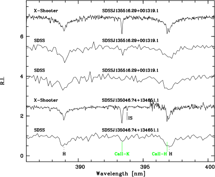
Figure 1: The SDSS spectra of the program stars in the region around the Ca ii K line compared to the X-Shooter spectra. The fact that this line is weaker than the neighbouring H lines is a diagnostic for extremely low metallicity. In the X-Shooter spectrum of SDSS J135046.74+134651.1 we labelled “IS” the weak interstellar Ca ii K line.

3 Observations and data reduction

Both stars were observed in visitor mode with the IFU in stare mode. In our case the use of the IFU was not aimed at obtaining any spatial information (the stars are point sources), but to collect as many photons as possible with resolution corresponding to that of a slit of 06, i.e. R=7900 in the UVB arm and R=12600 in the VIS arm. SDSS J135046.74+134651.1 was observed on April 7th 2010, with a single integration of 5400 s, in the IR arm the integration time was divided into 6 DITs of 900 s each. SDSS J135516.29+001319.1 was observed on May 17th 2010, with two integrations of 3150 s each, in the IR arm each integration was split into 4 DITs of 787 s. The different integrations were co-added. The spectra were reduced using the X-Shooter pipeline (Goldoni et al. 2006). The IR arm did not contain any useful information, the present paper is based on the analysis of the UVB and VIS arms. The UVB arm covers the range 300-559.5 nm and the VIS arm 559.5-1024 nm.

The signal to noise ratios achieved were S/N=37 at 415 nm and 38 at 660 nm for SDSS J135046.74+134651.1 and S/N=18 at 415 nm and 20 at 660 nm for SDSS J135516.29+001319.1.

3.1 Analysis

Our abundance analysis is based on 1D ATLAS model atmospheres. We began with atmospheres computed with version 9 of the ATLAS code (Kurucz 1993, 2005) on Linux (Sbordone et al. 2004; Sbordone 2005). In this version of ATLAS the line opacity is treated through Opacity Distribution Functions (ODFs) and we used the ones computed by Castelli & Kurucz (2003), for a microturbulent velocity of 1 $\mathrm{km\,s^{-1}}$. For SDSS J135516.29+001319.1, given that its abundance pattern is significantly different from that assumed in the computation of the ODFs, we also computed a specific model atmosphere with version 12 of the ATLAS code, which uses opacity sampling (Kurucz 2005; Castelli 2005a), and our final analysis is based on this model. Convection was treated in the mixing-length approximation with a mixing-length parameter $\alpha_{\mathrm{MLT}}$= 1.25.

We also used a 3D hydrodynamical model atmosphere (3D model here after) computed with the CO⁵BOLD code, (for details see Freytag et al. 2011) to compute 3D corrections. This CO⁵BOLD model has parameters T_eff/ log g/[M/H]=6320K/4.5/–2.0, and the series of 20 selected snapshots covers 2.5 h. As a reference 1D models we used two 1D model atmospheres, $\left\langle\mathrm{3D}\right\rangle$ and $\mathrm{1D}_{\mathrm{LHD}}$: $\left\langle\mathrm{3D}\right\rangle$ is obtained from the 3D model by averaging all snapshots horizontally at surfaces of equal Rosseland optical depth; $\mathrm{1D}_{\mathrm{LHD}}$ is computed with the code LHD, that employs the same microphysics and radiative transfer scheme as the CO⁵BOLD code. For both these models, in the spectral synthesis we used a microturbulence of 1.5$\mathrm{km\,s^{-1}}$, and the mixing-length parameter of the LHD model was fixed at 0.5.

The 3D corrections are defined as in Caffau et al. (2010), the difference of the abundance derived from the 3D model and the one derived from the 1D reference models: $\Delta_{\rm gran}={\rm A(X)_{\rm 3D}-A(X)_{\rm\left\langle\mathrm{3D}\right\rangle}}$ to isolate the granulation effects, due to horizontal fluctuations; $\Delta_{\rm LHD}={\rm A(X)_{\rm 3D}-A(X)_{\rm\mathrm{1D}_{\mathrm{LHD}}}}$ to measure the effects that both the horizontal fluctuation and the temperature structure have on the abundance determination.

In the spectrum synthesis we used the atomic parameters used in the “First Stars” survey (Cayrel et al. 2004; François et al. 2007; Bonifacio et al. 2009). The reference solar iron abundance 7.52 is from Caffau et al. (2010). For the other elements the solar reference is from Lodders et al. (2009).

We measured the equivalent widths (EW) of the lines in the observed spectra using the IRAF task splot and derived the abundance with the code WIDTH (Kurucz 2005; Castelli 2005b). We used the line positions of the lines used for the abundance analysis in the UVB spectrum to derive a radial velocity of the stars. The results are given in Table 1 along with the error on the mean of the velocities. We did not observe any radial velocity standards, thus we do not have a good estimate of the external error on these radial velocities. For star SDSS J135046.74+134651.1 the SDSS spectrum provides a radial velocity of $(-299\pm 24)$$\mathrm{km\,s^{-1}}$, compatible with our measurement at less than 2 $\sigma$. For star SDSS J135516.29+001319.1, there are two SDSS spectra, which provide $(-43\pm 34)$$\mathrm{km\,s^{-1}}$and $(-33\pm 30)$$\mathrm{km\,s^{-1}}$, although both measurements are compatible with ours, it is possible that the star is a radial velocity variable. These comparisons suggest that the external error is not larger than a few $\mathrm{km\,s^{-1}}$.

The large negative radial velocity of SDSS J135046.74+134651.1 allows to clearly resolve the interstellar Ca ii K line, as shown in Fig. 1. The line has an EW of 1.6 pm, such a weak line is expected, given the low reddening of this star. For star SDSS J135516.29+001319.1 the low radial velocity implies that the photospheric line is contaminated by the interstellar absorption, however, since this star has an even lower reddening, we expect the interstellar line to be even weaker, thus the contamination should be less than 1%.

4 SDSS J135046.74+134651.1

4.1 Stellar parameters

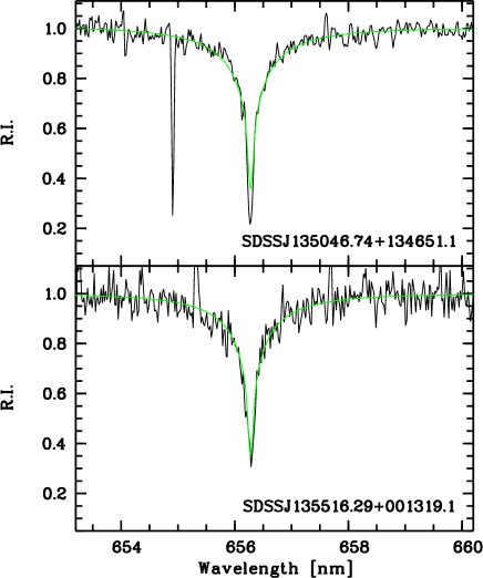
Figure 3: The X-Shooter spectrum of SDSS J135046.74+134651.1 (solid black) with the best fitting CO⁵BOLD profile (T_eff= 6420 K, solid green) in the top panel and the same for SDSS J135516.29+001319.1 (T_eff= 6288K̇, solid green) in the bottom panel.

From the $(g-z)_{0}$ colour we derived an effective temperature of 6284 K. The colour excess provided by the SDSS catalogue for this star is given in Table 1 and is is based on the reddening maps of Schlegel et al. (1998). It is very low and ignoring it would result in an effective temperature lower by 65 K. As a check, we also derived T_eff by fitting the H$\alpha$ wings. The theoretical profiles were computed using the self broadening theory of Barklem et al. (2000) and the Stark broadening of Stehlé & Hutcheon (1999). As done in Sbordone et al. (2010), we used the CIFIST grid of CO⁵BOLD models Ludwig et al. (2009), a grid of $\mathrm{1D}_{\mathrm{LHD}}$ models with a mixing length parameter of 0.5, a gravity of 4.5, and metallicity -2.0 and –3.0, and an analogous grid of ATLAS 9 models. From the CO⁵BOLD models we obtain a temperature of 6420 K (see Fig. 3), from the $\mathrm{1D}_{\mathrm{LHD}}$ models 6240 K, and from the ATLAS models 6400 K. The difference between $\mathrm{1D}_{\mathrm{LHD}}$ and ATLAS models is not surprising, given the different temperature structures of the models. The photometric and H$\alpha$-based temperatures are consistent within $\sim 100$ K, and each of them has an associated error which is again of about 100 K. Moreover, the accuracy of the present analysis is limited mainly by the limited S/N ratio and resolution of the spectra, rather than by the temperature uncertainty. We thus decided to adopt the photometric temperature. The gravity has been fixed at log g= 4.5, based on the Fe i and Fe ii equilibrium. The resolution of X-Shooter, even with the IFU, and the achieved S/N ratio, do not allow to measure weak lines, on the linear part of the curve of growth. Therefore the microturbulence cannot be derived from the observation. This parameter is not a really independent parameter in 1D analysis, and it can be calibrated as a function of effective temperature and, mainly, surface gravity. We decided to apply the relation of Edvardsson et al. (1993) which yields a microturbulence of 1.5 $\mathrm{km\,s^{-1}}$. It must be noted that in this way microtrubulence and surface gravity are strictly correlated. Any change in surface gravity implies a change in microturbulence, which implies a change in the abundances of both Fei and Feii, and thus a change in gravity. Therefore the finally adopted values had to be determined iteratively.

4.2 Abundances

The derived abundances are given in Table 2, while in Table 4 all the lines considered are listed with the atomic parameters, the equivalent width (EW), the abundance derived from the photometric temperature and from the H$\alpha$ 3D best fit, the 3D corrections, and the abundance derived after applying the 3D corrections.

The star is metal-poor, [Fe/H]$=-2.3$, but not around $-3.0$, as expected from the analysis of the SDSS spectrum. The striking thing is that the iron content is similar to the abundance of $\alpha$-elements. This is unusual because the metal-poor Halo stars display generally an enhanced abundance of $\alpha$-elements. This expected overabundance of $\alpha$-elements is in fact folded into our method of analysis of SDSS spectra where metallicity is derived also from lines of $\alpha$-elements. In fact at low metallicity the dominant feature is the Ca ii K line. It is thus not surprising that such a non-$\alpha$ enhanced star is estimated to have a too low iron abundance from the SDSS spectra.

The elements detectable in the observed spectrum are Fe (both Fe i and Fe ii), Mg, Si, and Ca (both neutral and singly ionised).

Table 2: Chemical abundances from the 1D ATLAS abundance analysis of SDSS J135046.74+134651.1.

El.	[X/H]	[X/H]	N†	${\rm A_{\odot}^{\ddagger}}$
	${\rm T_{\rm eff}}=6284$ K	${\rm T_{\rm eff}}=6420$ K
Mg i	$-2.30\pm 0.06$	$-2.15\pm 0.06$	2	7.54
Si i	$-2.54$	$-2.43$	1	7.52
Ca i	$-2.15$	$-1.99$	1	6.33
Ca ii	$-2.21\pm 0.21$	$-2.12\pm 0.19$	4	6.33
Fe i	$-2.33\pm 0.20$	$-2.17\pm 0.20$	12	7.52
Fe ii	$-2.28$	$-2.25$	1	7.52

^† Number of lines
^‡ A(X) = log(X/H) + 12

We apply the 3D corrections, $\Delta_{\rm LHD}$, to the 1D analysis based on the temperature derived from the photometry. $\Delta_{\rm LHD}$ corrections are negative, meaning that the abundance derived from 3D model atmosphere is smaller than the one derived from 1D reference model. This is due to the fact that hydrodynamical models are usually cooler than hydrostatical models in the outer part of the atmosphere. The lines formed in the outermost layers are thus more affected by the cooling effect. Usually lines of neutral elements with low excitation energy, show the largest effects. $\Delta_{\rm gran}$ is close to zero, meaning that for the observed lines the horizontal fluctuations do not play a determinant role, the strongest effect is of almost 0.2 dex for the line of Fe ii.

4.3 Li abundance

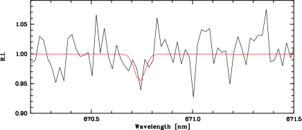
Figure 2: The fit of the Li doublet at 670.7 nm with a grid of ATLAS+SYNTHE profiles. As evident from the feature on the blue side of the Li, the Li line is comparable with the noise of the spectrum.

The Li feature at 670.7 nm is not detected, its EW being at the level of the noise, so that we consider the abundance derived as an upper limit. With a 1D grid of ATLAS+SYNTHE synthetic profiles we fitted the observed profile (see Fig.2). We determined the EW of the best fit and used this EW to derive the 3D-NLTE abundance of Li by using the fitting function of Sbordone et al. (2010), which yields A(Li)=2.38. This value is compatible with the level of the Spite plateau (Spite & Spite 1982; Sbordone et al. 2010).

5 SDSS J135516.29+001319.1

5.1 Stellar parameters

The effective temperature from the $(g-z)_{0}$ colour is extremely high, T_eff=6765 K. Also for this star the reddening (see Table 1) is low, ignoring the reddening correction would provide a temperature which is only 106 K lower, therefore still extremely high. According to published stellar isochrones, such a hot star should be very young, unless it is a Blue Straggler star, or lies on the Horizontal Branch. We note however that the evolutionary tracks of Piau et al. (2006), computed with CNO enhanced chemical composition, predict such a hot Turn-Off for a population of 12 Gyrs. The colours of this star could in fact suggest a CNO-enhanced metal-poor star.

The 3D fit of the H-$\alpha$ profile gives a considerably lower effective temperature of 6300 K. Among the other colours, $(g-r)_{0}$ and $(r-i)_{0}$ support the high T_eff indicated by $(g-z)_{0}$; the $(i-z)_{0}$ colour is considerably sensitive to the surface gravity, it supports the high temperature for log g= 4.5, but for log g=4.0 it implies T_eff=6300 K.

We therefore decided to adopt an effective temperature of 6300 K, which is consistent with the Halo Turn-Off. The iron ionisation equilibrium implies log g= 3.9 and the microturbulence derived from the Edvardsson et al. (1993) calibration is 2.3 $\mathrm{km\,s^{-1}}$. We note that the inconsistency between colour and H$\alpha$, as well as the possible inconsistency of $(g-z)_{0}$ and $(i-z)_{0}$, is a hint of a peculiar spectral energy distribution.

5.2 Abundances

The abundances derived assuming both effective temperatures (photometric and H$\alpha$) are provided in Table 3. Among the $\alpha$ elements Si and Mg appear underabundant with respect to iron, but it should be noted that the measurement is based on a single line for each of the two elements. Given this unusual chemical composition, different from the ones available in the ODFs computed by Castelli & Kurucz (2003), and the importance of Mg as electron donor, we computed models with version 12 of the ATLAS code, using the desired chemical composition. The abundances were then recomputed with this new model. The differences with respect to those obtained from an ATLAS model computed with version 9 and non-$\alpha$-enhanced ODFs are very small. At these low metallicities and high gravities, even consistent variations of Mg abundance have minor effects on the model structure.

The Ca ii abundance in Table 3 is based on two lines of the IR triplet. It must be remarked that the Ca ii K line is not compatible with this abundance and is consistent with a Ca abundance which is lower by 0.7 dex. Since the Ca ii K line is the main abundance indicator at low metallicity for the SDSS spectra, this explains why we had estimated a much lower metallicity than what results from the analysis of the X-Shooter spectrum. Also the Ca i line, implies an abundance which is 0.5 dex higher than the Ca ii IR triplet. It should be noted that according to the NLTE computations of Mashonkina et al. (2007) the corrections for Ca ii triplet lines are always negative, those for Ca i 4226̇  nm are always positive. Thus the cause of this discrepancy should not be due to NLTE effects, which would rather tend to increase the discrepancy.

We could not convincingly detect the Li i 670.7 nm feature. The EW upper limit is 5.4 pm corresponding to A(Li)$<$2.98 at a temperature of 6765 K and 2.63 at 6300 K.

We inspected carefully the spectrum for any sign of carbon enhancement, looking at the G-band and all the C i lines which are observed in carbon-enhanced metal-poor stars (see e.g. Behara et al. 2010), but could not detect any.

Table 3: Chemical abundances from the 1D ATLAS abundance analysis for SDSS J135516.29+001319.1.

El.	[X/H]	[X/H]	N	${\rm A\odot}$
	${\rm T_{\rm eff}=6765}$ K	${\rm T_{\rm eff}=6300}$ K
Mg i	$-1.85$	$-2.08$	1	7.54
Al i	$-1.34$	$-1.66$	1	6.47
Si i	$-1.95$	$-2.19$	1	7.52
Ca ii	$-1.31\pm 0.25$	$-1.59\pm 0.03$	2	6.33
Ti ii	$-0.84\pm 0.53$	$-1.33\pm 0.49$	7	4.90
Cr i	$-0.82$	$-1.39$	1	5.64
Fe i	$-1.29\pm 0.31$	$-1.74\pm 0.39$	12	7.52
Fe ii	$-1.40\pm 0.27$	$-1.78\pm 0.30$	3	7.52
Sr ii	$-1.11\pm 0.20$	$-1.65$	1	2.92
Ba ii	$-1.52$	$-2.10$	1	2.17

6 Discussion

These first observations of metal-poor SDSS candidates with X-Shooter allows us to estimate the strengths and limitations of this instrument for this application. The great strength is the high efficiency of X-Shooter, which has allowed us to obtain a workable spectrum of a star of 19th magnitude in less than two hours. The use of the IFU (Guinouard et al. 2006) as image slicer has been successful. The transmission of the IFU in the UVB arm is lower than at longer wavelengths. The opportunity of using the IFU rather than a slit of 06 depends of course on the seeing. In the case of the observations described here the seeing was always between 10 and 12, the advantage of using the IFU is unquestionable.

The main limitation of X-Shooter for abundance analysis is the resolution, which is too low to allow us to measure lines on the linear part of the curve of growth. Lines on the flat part of the curve of growth are little sensitive to abundance, so that a large error is always associated to abundances derived from such lines. The situation is better for lines which are even stronger and lie in the damping part of the curve of growth, although in this case the damping parameters should be accurately known. For metal-poor dwarf stars, however, even the Ca ii K line has weak wings and is usually on the flat part of the curve of growth. A partial compensation is provided by the very large spectral coverage provided by X-Shooter, which allows to measure many features, improving the abundance accuracy. This, however, for metal poor stars, applies only to iron, since the other species are represented by only one or few lines.

The two stars studied in these first GTO runs did not turn out to be as metal-poor as expected from the analysis of the SDSS spectra, the main reason being, in both cases, the weakness of the Ca ii K line with respect to the iron lines. In fact our analysis of SDSS spectra estimates the metallicity by using all available features assuming that $\alpha$ elements are enhanced by 0.4  dex over iron.

In the case of SDSS J135046.74+134651.1, for the few measurable elements, the abundances appear to be solar-scaled. The existence of metal-poor stars with low, almost solar $\alpha$ to iron ratios was pointed out by Nissen & Schuster (1997), however, the most metal-poor stars of that sample had a metallicity about –1.0. Remarkable known metal-poor $\alpha$-poor stars are BD+ 80^∘ 245, with a metallicity of –1.8 and a logarithmic $\alpha$ to iron ratio of –0.3 (Carney et al. 1997) and CS 22873-139 (Spite et al. 2000) with a metallicity of –3.4, [Mg/Fe]=–0.04, [Ca/Fe]=+0.16 and [Ti/Fe]=+0.55. The latter star is a double spectrum spectroscopic binary. At lower metallicities stars with bizarre compositions are known, such as HE 1424-0241 (Cohen et al. 2007), with a metallicity around –4.0 and Si underabundant by 1 dex, but magnesium “normally” enhanced, or SDSS J234723.64+010833.4 (Lai et al. 2009) which has a small underabundance of Mg ([Mg/Fe]=–0.1) but a strong overabundance of Ca ([Ca/Fe]=+1.1), at a metallicity of –3.2.

SDSS J135046.74+134651.1 appears to have an abundance pattern similar to BD+ 80^∘ 245, and CS 22873-139. The most straight forward interpretation of these $\alpha$–poor metal–poor stars is that they were formed in low-mass galaxies, satellites of the Milky Way, characterized by a low or bursting star-formation rate. The original galaxies have been disrupted due to tidal interaction, and their debris populates the Halo. It is interesting to point out that the surviving satellite galaxies have indeed low $\alpha$ to iron ratios, although only Carina displays essentially solar $\alpha$ to iron ratios at a metallicity around –2.0 (see the review of Tolstoy et al. 2009). However, at even lower metallicity ([Fe/H]=$\sim$3 and below), solar-scaled $\alpha$ element abundances are detected in stars of Sculptor and Sextans dSph (Tafelmeyer et al. 2010). Thus, in a naive interpretation, the majority of surviving satellites had a higher star formation rate than Carina, Sculptor, Sextans or the disrupted satellites, such as the one in which SDSS J135046.74+134651.1 originated. A more extensive survey searching for EMP stars in the halo may allow us to quantify the percentage of these low-$\alpha$ stars.

The case of SDSS J135516.29+001319.1 is less clear. The discrepancy, in terms of T_eff, between several colours and H-$\alpha$ strongly suggests that the spectral energy distribution is anomalous. It would be tempting to suggest the presence of a companion emitting a considerable flux in the UV. The most likely candidate is a hot white dwarf, however it should be about four magnitudes fainter than the Turn-Off star, thus its effect would be negligible. The situation could be different if the white dwarf were surrounded by an accretion disc providing a significant UV continuum. We are entering here in the domain of the wild speculation, and not enough observational data are available to enable us to present a consistent hypothesis. The weakness of the Ca ii K line with respect to the Ca ii IR triplet could in fact be explained by the presence of excess UV flux, however this could not explain the unusual strength of the Ca i resonance line, which is only 29 nm to the red of Ca ii K. It is also possible that we are observing a binary system composed of two stars, of different T_eff  one could immagine the cooler companion to contribute the Ca ii IR triplet and the Ca i lines, while the warmer one contributes the Ca ii K line. In this case however the measurements suggest a T_eff  difference of at least 1000 K, thus the luminosities of the two companions have to be carefully chosen, in order to provide the observed spectrum. The quality of the available data is not sufficient to explore such composite spectrum solutions. We conclude that this star has a peculiar spectrum, possibly composite and its abundances ought to be regarded as highly uncertain. Further radial velocities measurements could allow to decide if the star is a binary.

We want to stress that the unique efficiency of X-Shooter opens up the possibility to measure the chemical abundances of the outer Halo in situ. To estimate the distances we used the SDSS photometry and the Padova isochrone of 13 Gyr and metallicity –2.0 (Marigo et al. 2008). The distances (averaged over all five SDSS bands) are 3.9 Kpc for SDSS J135046.74+134651.1 and 9.1 Kpc for SDSS J135516.29+001319.1, they are likely the most distant dwarf stars for which the detailed chemical composition could be measured. We used the Besançon Galactic model (Robin et al. 2003) to simulate a field of stars with colours and magnitudes similar to our own. In the field around SDSS J135046.74+134651.1, the distribution of radial velocities has mean of 0$\mathrm{km\,s^{-1}}$with a dispersion of 80 $\mathrm{km\,s^{-1}}$, confirming that the star, with radial velocity -331 $\mathrm{km\,s^{-1}}$, has little to do with the Halo, and strengthening the hypothesis of its extra-Galactic origin. Instead in the case of SDSS J135516.29+001319.1 its nearly zero radial velocity is perfectly consistent with the mean radial velocity of Halo stars in this field.

Appendix A Appendix A

Table 4: Abundance from each line, from the 1D ATLAS+WIDTH, and 3D corrections for SDSS J135046.74+134651.1.

Element	$\lambda$	$\xi$	$\log\,gf$	EW†	$\Delta_{\rm gran}$	$\Delta_{\rm LHD}$	[X/H]	[X/H]	[X/H]
		eV		[pm]			${\rm T_{\rm eff}}$ K	${\rm T_{\rm eff}}$ K	${}_{\rm 1D}+\Delta_{\rm gran}$
							=6284	=6420
Fe i	381.5840	1.485	0.237	16.1	–0.03	–0.21	–1.96	–1.78	–2.17
Fe i	382.0425	0.860	0.119	15.0	–0.09	–0.33	–2.47	–2.28	–2.80
Fe i	385.6371	0.052	–1.286	10.6	–0.14	–0.56	–2.30	–2.11	–2.86
Fe i	386.5523	1.011	–0.982	8.6	0.00	–0.34	–2.17	–2.01	–2.51
Fe i	404.5812	1.485	0.280	11.8	0.03	–0.26	–2.48	–2.31	–2.75
Fe i	406.3594	1.557	0.062	9.9	0.04	–0.28	–2.51	–2.35	–2.79
Fe i	413.2058	1.608	–0.675	7.0	–0.05	–0.32	–2.40	–2.26	–2.72
Fe i	414.3868	1.557	–0.511	8.2	–0.01	–0.33	–2.36	–2.22	–2.69
Fe i	426.0474	2.399	0.109	6.8	0.00	–0.18	–2.40	–2.28	–2.59
Fe i	438.3545	1.485	0.200	10.6	0.03	–0.33	–2.65	–2.49	–2.98
Fe i	440.4750	1.557	–0.142	10.5	0.03	–0.34	–2.26	–2.10	–2.61
Fe i	495.7596	2.808	0.233	8.5	0.04	–0.21	–2.03	–1.90	–2.22
Fe ii	516.9033	2.891	–0.870	7.7	0.18	0.16	–2.28	–2.25	–2.12
Mg i	517.2684	2.712	–0.380	15.0	–0.02	–0.21	–2.36	–2.21	–2.57
Mg i	518.3604	2.712	–0.158	20.0	0.00	–0.21	–2.24	–2.08	–2.46
Si i	390.5523	1.909	–1.090	8.9	0.06	–0.16	–2.54	–2.43	–2.70
Ca i	422.6728	0.000	0.240	14.1	–0.10	–0.42	–2.15	–1.98	–2.57
Ca ii	393.3663	0.000	0.134	159.5	–0.05	–0.19	–2.46	–2.31	–2.65
Ca ii	849.8023	1.692	–1.312	22.1	0.09	–0.25	–1.92	–1.85	–2.17
Ca ii	854.2091	1.700	–0.362	36.2	0.01	–0.20	–2.35	–2.27	–2.55
Ca ii	866.2141	1.692	–0.623	35.3	0.02	–0.21	–2.11	–2.05	–2.32

^† The relative errors on EWs are of the order of 25%.

References

- Adelman-McCarthy et al. (2008) Adelman-McCarthy, J. K., et al. 2008, ApJS, 175, 297
- Barklem et al. (2000) Barklem, P. S., Piskunov, N., & O’Mara, B. J. 2000, A&A, 363, 1091
- Behara et al. (2010) Behara, N. T. et al. 2010, A&A, 513, A72
- Bonifacio & Caffau (2003) Bonifacio, P., & Caffau, E. 2003, A&A, 399, 1183
- Bonifacio et al. (2009) Bonifacio, P. et al. 2009, A&A, 501, 519
- Caffau et al. (2010) Caffau, E. et al. 2010, Solar Physics 66
- Carney et al. (1997) Carney, B. W. et al. 1997, AJ, 114, 363
- Castelli (2005a) Castelli, F. 2005, MSAIS 8, 25
- Castelli (2005b) Castelli, F. 2005, MSAIS 8, 44
- Castelli & Kurucz (2003) Castelli, F. & Kurucz, R. L. 2003, in IAU Symposium, ed. N. Piskunov, W. W. Weiss, & D. F. Gray, 20P, arXiv:astro-ph/0405087v1
- Cayrel et al. (2004) Cayrel, R., et al. 2004, A&A, 416, 1117
- Cohen et al. (2007) Cohen, J. G. et al. 2007, ApJ, 659, L161
- D’Odorico et al. (2006) D’Odorico, S., et al. 2006, Proc. SPIE, 6269E, 98
- Edvardsson et al. (1993) Edvardsson, B. et al. 1993: A&A 275, 101
- François et al. (2007) François, P., et al. 2007, A&A, 476, 935
- Freytag et al. (2011) Freytag, B. et al. 2011, “Realistic simulations of stellar convection”, Journal of Computational Physics: special topical issue on computational plasma physics, ed. Barry Koren
- Goldoni et al. (2006) Goldoni, P., Royer, F., François, P., Horrobin, M., Blanc, G., Vernet, J., Modigliani, A., & Larsen, J. 2006, Proc. SPIE, 6269, 80
- Guinouard et al. (2006) Guinouard, I.et al. 2006, Proc. SPIE, 6273E, 116
- Kurucz (1993) Kurucz, R. 1993: ATLAS9 CD-ROM No. 13. Cambridge, Mass.: Smithsonian Astrophysical Observatory, 1993., 13
- Kurucz (2005) Kurucz, R. L. 2005: MSAIS 8, 14
- Lai et al. (2009) Lai et al. 2009, ApJ, 697, L63
- Lodders et al. (2009) Lodders, K., Palme, H., & Gail, H.P.: 2009, “Abundances of the elements in the solar system”, Landolt-Börnstein, New Series, Vol. VI/4B, Chap. 4.4, J.E. Trümper (ed.), Berlin, Heidelberg, New York: Springer Verlag, p. 560-630
- Ludwig et al. (2008) Ludwig, H.-G. et al. 2008, Physica Scripta Volume T, 133, 014037
- Ludwig et al. (2009) Ludwig, H.-G. et al. 2009, Mem. Soc. Astron. Italiana, 80, 711
- Marigo et al. (2008) Marigo, P., et al/ 2008, A&A, 482, 883
- Mashonkina et al. (2007) Mashonkina, L., Korn, A. J., & Przybilla, N. 2007, A&A, 461, 261
- Nissen & Schuster (1997) Nissen, P. E., & Schuster, W. J. 1997, A&A, 326, 751
- Piau et al. (2006) Piau, L. et al. 2006, ApJ, 653, 300
- Robin et al. (2003) Robin, A. C. et al. 2003, A&A, 409, 523
- Sbordone et al. (2004) Sbordone, L., Bonifacio, P., Castelli, F., & Kurucz, R. L. 2004: MSAIS 5, 93
- Sbordone (2005) Sbordone, L. 2005, MSAIS 8, 61
- Sbordone et al. (2010) Sbordone, L., et al. 2010: A&A 522, A26
- Schlegel et al. (1998) Schlegel, D. J., Finkbeiner, D. P., & Davis, M. 1998, ApJ, 500, 525
- Spite & Spite (1982) Spite, M., & Spite, F. 1982, Nature, 297, 483
- Spite et al. (2000) Spite, M., et al. 2000: A&A 360, 1077
- Stehlé & Hutcheon (1999) Stehlé, C., & Hutcheon, R. 1999, A&AS, 140, 93
- Tafelmeyer et al. (2010) Tafelmeyer, M., et al. 2010, A&A, 524, A58
- Tolstoy et al. (2009) Tolstoy, E., Hill, V., & Tosi, M. 2009, ARA&A, 47, 371
- York et al. (2000) York, D. G., et al. 2000, AJ, 120, 1579