Kinematic Evolution of a Slow CME in Corona Viewed by STEREO-B on 8 October 2007

Abstract

We studied the kinematic evolution of the 8 October 2007 CME in the corona based on Sun-Earth Connection Coronal and Heliospheric Investigation (SECCHI) onboard satellite B of Solar TErrestrial RElations Observatory (STEREO). The observational results show that this CME obviously deflected to a lower latitude region for about 30^∘ at the beginning. After this, the CME propagated radially. We also analyze the influence of the background magnetic field on the deflection of this CME. We find that the deflection of this CME at an early stage may be caused by the nonuniform distribution of the background magnetic field energy density and that the CME tended to propagate to the region with lower magnetic energy density. In addition, we found that the velocity profile of this gradual CME shows multiphased evolution during its propagation in COR1-B FOV. The CME velocity first kept at a constant of 23.1km.s^-1. Then, it accelerated continuously with a positive acceleration of $\approx$7.6m.s^-2.

1 Introduction

Some parameters of CMEs may greatly change during their propagation in the corona. The variation of the CME’s propagation parameters during this phase could significantly influence the CME’s geoeffectiveness: (i) the propagation direction variation would determine whether a CME could arrive on Earth; (ii) the evolution of CME’s velocity may change the CME’s arrival time. Thus, the study of the kinematic evolution of the CME in the corona is an important topic in space physics, especially for space weather study.

The CME deflection in the meridian plane during its propagation in the corona has been reported by many authors. MacQueen, Hundhausen, and Conover [1986] found that there was an average 2.2^∘ Equator – ward deflection of the CMEs in the Skylab epoch (1972  –  1974) during solar minimum. Cremades and Bothmer [2004] studied the differences between the central position angle (CPA) and the source region position angle and found that the CME deflected to lower latitude region by about 20^∘ after solar minimum. This type of deflection would make the CME, which originated from a high latitude region, propagate to the ecliptic plane and subsequently encounter Earth. Based on a STEREO observation, Kilpua et al. [2009] showed such an example:2 November 2008 CME. However, the causes for this deflection are still debated. Previous authors suggested that two factors would cause this deflection of the CME: (i) the influence of the background coronal magnetic field [MacQueen, Hundhausen, and Conover, 1986]; (ii) the fast solar wind flow from polar coronal holes that encompassed the CMEs’ expansion at higher latitude [Cremades, Bothmer, and Tripathi, 2006].

Another important factor that would influence the CME’s space weather effect is the velocity evolution of the CME, especially when the CME propagates in the corona where the major acceleration of CMEs take place [Zhang et al., 2004]. Previous results showed that CMEs usually undergo a multiphased kinematic evolution, including (i) the initiation phase, (ii) the impulsive (major) acceleration phase and (iii) the propagation phase [Zhang et al., 2001, 2004]. However, not all CMEs necessarily display a full three – phase evolution. A class of gradual CMEs characterized by a very weak but long duration acceleration has also been reported [Sheeley et al., 1999; Srivastava et al., 1999, 2000]. Based on the different acceleration properties, Zhang et al. [2004] suggested that there were three classes of CMEs: (i) impulsive acceleration CMEs; (ii) intermediate acceleration CMEs; (iii) gradual acceleration CMEs.

Recently, the twin Solar TErrestrial RElations Observatory (STEREO) spacecraft [Kaiser et al., 2007], which was launched on 25 October 2006, provide the observations of CMEs with higher resolution and larger range. The COR1 instrument [Howard et al., 2008] on SECCHI observed the Sun from 1.5 – 4.0 $R_{\odot}$ with a time cadence of five minutes, and the COR2 instruments observed the Sun from 2.0 – 15 $R_{\odot}$ with a time resolution of 15 minutes. The COR1 design is the first space – borne internally occulted refractive coronagraph [Howard et al., 2008] and COR2 imaged the corona with five times the spatial resolution and three times the temporal resolution of LASCO/C3 . Thus, the combination of COR1 and COR2 observations can be used to study the CME’s kinematic evolution in the corona with high spatial and time resolution.

We will study the kinematic evolution including the propagation direction variation and the velocity evolution of the 8 October 2007 CME during its propagation from $\approx$2.0 to $\approx$10$R_{\odot}$ based on the COR1-B and COR2-B observations (B denotes that it is on the STEREO B spacecraft). This was a very slow CME with a speed that varied from $\approx$20km.s^-1 to $\approx$90km.s^-1 during its propagation in the COR1-B and COR2-B FOV. Because the CME was very slow, COR1-B recorded $\approx$100 images. This large number of frames provides us with an opportunity to study the CME’s kinematic evolution during its propagation in the corona. The detailed observations of this CME will be shown in Section 2. In Section 3 the influence of background magnetic field on the deflection of this CME will be studied in detail by an analytical method. In the last section, we will give our conclusion and discussion.

2 Observations

The CME was firstly recorded by COR1-B at 08:46 UT on 8 October 2007. The panels in Figure 1 show the COR1-B and COR2-B observations of this CME.

Seen from STEREO B, this CME first appeared at solar west limb. A burst prominence starting at about 07:00 UT on 8 October, as seen by EUVI-B 304Å, was associated with this CME. Because the CME was launched from the western limb and showed a helical circular – like structure, this suggests that the CME was viewed by the instruments through an axial – view angle [Cremades and Bothmer, 2004; Wang, Zhang, and Shen, 2009]. Therefore, the projection of the CME onto the plane of the sky can be treated as the cross – section of the CME. Wang, Zhang, and Shen [2009] studied the internal state of this CME based on its expansions and propagations from STEREO-B observations. Note that this slow and weak CME became diffused when it propagated in the later stage of COR1B FOV (from $\approx 3R_{\odot}$ to $\approx 5R_{\odot}$) as shown in Figure 1(f). Thus, some of the CME’s parameters can’t be measured correctly during this period. For this reason, these images were excluded from the analysis below. After the CME propagated into COR2B FOV, it represent a clear structure as panels (g) – (i) in Figure 1 shown. Finally, a total of 67 images in COR1 FOV and 14 images in COR2 FOV were used.

2.1 Deflected Propagation in the Meridian Plane

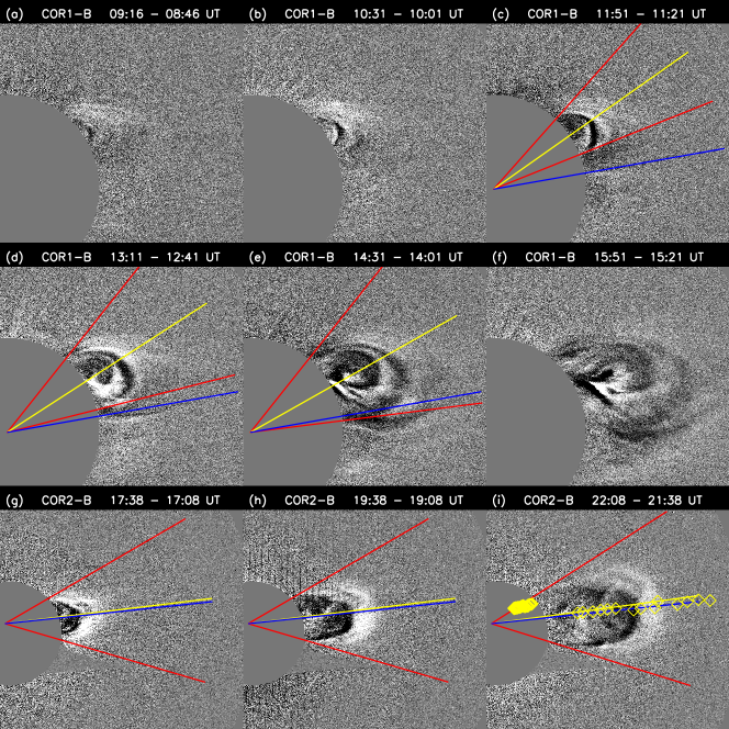
Figure 1: Images of 8 October 2007 CME taken by STEREO/SECCHI COR1-B (a – f) and STEREO/SECCHI COR2-B (g – i). The red lines in panel (c) – (e) and (g) – (i) show the selected maximum and minimum position angle of the CME while the yellow lines show the radial direction of the CME’s CPA. The blue lines in these panels show the line with a position angle of 276^∘. The yellow symbols in panel (i) show the variation of the CPA of the CME.

The COR1-B and COR2-B observations of this CME are shown in Panels (a) – (f) and (g) – (i) in Figure 1, respectively. The red lines in panel (c) – (e) and (g) – (i) show the selected maximum and minimum position angle of the CME while the yellow lines in these panels show the radial direction of the CME’s CPA. The yellow symbols in panel (i) show the variation of the CPA of the CME. The CME is too weak at the beginning as shown in panel (a) and (b) while the CME was diffused at later stage of COR1-B FOV shown as panel (f) shown. So, no position angle was measured during these period. The panels (a) – (f) in Figure 1 show that the CME obviously propagated non-radially during its propagation in the COR1-B FOV. At this stage, this CME deflected to Equator. After the CME propagated into the COR2-B FOV, no obvious deflection could be found from panels (g) – (i) in Figure 1.

Figure 2: CME central angle position (CPA) varied with CME leading edge height. The crosses and diamonds denote the observations of COR1-B and COR2-B respectively. The triangles show the position angles of the heliospheric neutral line at different heights at the same Carrington longitude as the CME propagation on the meridian plane.

Figure 2 shows the central position angles (CPAs) of this CME varied with its leading edge heights (LEHs). The central position angle (CPA) is defined as the middle position angle with respect to the two edges of the CME in the sky plane, and the position angle (PA) is measured counterclockwise from solar North in degrees [Yashiro et al., 2004]. The crosses in Figure 2 show the COR1-B observations, while the diamonds show the observations of COR2-B. Note that there is a data gap. This data gap appeared because this slow and weak CME became diffused when it propagated from $\approx$3.0 to $\approx$5.0 $R_{\odot}$, as we discussed above. The COR1 observations show that this CME continuously deflected to the Equator at the early stage. During this stage, the CPA of this CME varied from $\approx 306^{\circ}$ to $\approx 294^{\circ}$. Then, this CME could continuously deflect to the Equator. After propagating to beyond $\approx$5.5$R_{\odot}$, the CME propagated almost radially along the line with a position angle of $\approx$276^∘ as the blue lines shown in Figure 1. Thus, the observational results show that this CME deflected to the Equator at the early stage and then propagated almost radially.

2.2 Multiple – phase Evolution of Velocity

Figure 3: Kinematic plots of the 8 October 2007 CME. The left panel shows the height – time plot and the right panel show the velocity – time plot. The solid lines show the line – fitting result of the height – time distribution of phase 1. The dotted – dashed lines show the second order fitting result with constant acceleration in phase 2. $V_{1}$ denotes the linear fit velocity of this CME at the first stage. The $V_{2}$ and $a_{2}$ denote the second order fit results of the velocity and acceleration in second phase.

Wang, Zhang, and Shen [2009] showed the velocity evolution of this CME in interplanetary space from its burst to the propagation to the place beyond 70 $R_{\odot}$. This is a gradual CME with a weak but long – duration acceleration. The list of the solar event report generated by NOAA/SEC indicated that no major solar flare was associated with this event. It was consistent with the result suggested by Zhang and Dere [2006] that CMEs without flares usually show gradual properties with a weak but long – duration acceleration.

Based on the COR1-B observations, the height – time and velocity – time evolutions of this CME during its propagation in the COR1 FOV are shown by diamonds in Figure 3(a) and crosses in Figure 3(b) respectively. The velocity measurements in Panel (b) were obtained by using the twelve – points running straight – line fitting method on HT measurements similar as in Sheeley et al. [1997]. At the beginning, the velocity of this CME is kept at a constant before the time of $\approx$11:30 UT (phase 1). The hight – time measurements during this phase can be well fitted by a straight line. The fitting result of the velocity at this phase is $\approx$23.1km.s^-1. After the time of 11:30 UT, the speed of the CME continuously and gradually increased (phase 2). The dotted – dashed lines in Figure 3 show the second order fitting result based on the height – time measurements with a constant acceleration. The fitting result correlates well with the observations. The acceleration of the CME during this phase was 7.6m.s^-2. This velocity profile shows that a CME with this gradual acceleration goes through a multiphased velocity evolution.

3 The Influence of the Background Magnetic Field on the CME’s Deflection

3.1 General Idea

The deflected propagations of CMEs and their driven shocks could be interpreted as the results of the interaction of the CMEs with the background solar wind and the magnetic field [e. g. MacQueen, Hundhausen, and Conover, 1986; Wei and Dryer, 1991; Gopalswamy et al., 2004]). So far, no theoretical analysis has been done to quantitatively study how the direction and magnitude of these deflections are influenced by background magnetic field. Therefore, we propose a simple method to discuss the CME’s deflection. Consider that a CME propagates in the coronal medium, the background magnetic field is perturbed by the CME, and the field lines that originally were in the region occupied by the CME are expelled. Compared with the unperturbed corona, the expelled magnetic field lines go around the CME and become significantly compressed, which means lots of free magnetic energy is built-up. The free energy from the compression provides a restoring force that acts on the CME. Since the background magnetic field is not uniformly distributed, the restoring forces acting on the different areas of the CME should not be the same. Therefore, the deflection may happen through the effect of the resultant force.

Consider a simple case as shown in Figure 4, in which we study the region occupied by the CME as an upper part and a lower part. The free energy corresponding to the upper part can be approximated as the original magnetic energy in it, i.e., $W_{U}\approx\int\omega\mathrm{d}x^{3}\approx\overline{\omega}_{U}\Delta V_{U}$, where $\omega=\frac{B^{2}}{2\mu}$ is the energy density and $\overline{\omega}_{U}$ is the average energy density in the upper part. The associated restoring force acting on the upper part points downward and is roughly given by $f_{U}\approx\frac{W_{U}}{L_{U}}$, where $L_{U}$ is the characteristic length of the part. Similarly, there is a restoring force acting on the lower part, which points in the opposite direction. Comparing the two forces, we can estimate the direction toward which the CME will propagate.

The above scenario can be easily extended to a more general situation. The net force acting on the CME is $f=f_{U}-f_{L}\approx\frac{W_{U}}{L_{U}}-\frac{W_{L}}{L_{L}}$. Obviously, its generalized form is

$$\textbf{f}=-\nabla\omega=-\nabla\left(\frac{B^{2}}{2\mu}\right).$$ (1)

Since we only know the CME’s deflected propagation in the latitudinal direction, it is not necessary to use Equation (1), and we just apply it as in the simple case given in the last paragraph.

Furthermore, we simply assume $\Delta V_{U}=\Delta V_{L}=\Delta V$ and $L_{u}=L_{L}=L$. Accordingly, the net force that acts on the CME can be rewritten as

$$f=\frac{\Delta V}{L}(\omega_{U}-\omega_{L})=\frac{\Delta V}{L}\Delta\omega,$$ (2)

where $\Delta\omega=\omega_{U}-\omega_{L}$ is the difference of the magnetic energy density between the upper and lower part. Based on Equation (2), a positive value of $\Delta\omega$ indicates that the CME – perturbed magnetic field will act an Equator – ward force on the CME, while a negative value of $\Delta\omega$ means an polar – ward force would act on the CME.

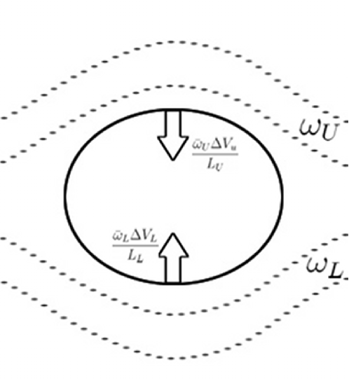
Figure 4: Sketch map of the CME – perturbed background magnetic field.

3.2 Calculated vs. observed Results

Figure 5: Distribution of the magnetic energy density ($\omega$) of the Carrington rotation 2061 at the hight of 3 $R_{\odot}$. The dashed line shows the neutral line at this height. The black cross shows the position of this CME at the hight of 3 $R_{\odot}$. The regions enclosed by the dotted – dashed line and the solid line shows the selected upper and lower part, respectively.

To apply this method, the background magnetic energy density should be given. However, there is no direct measurement of the solar magnetic field except at the photosphere up till now. The three – dimension(3D) magnetic field of the solar corona could only be calculated by different models. In this work, the magnetic energy density will be calculated from the 3D magnetic field extrapolated by the Current Sheet – Source Surface (CSSS) model. The CSSS model was developed by Zhao and his colleagues [Zhao and Hoeksema, 1995; Zhao, Hoeksema, and Rich, 2002]. This model has been used to reproduce the magnetic field strength at 1AU [Zhao, Hoeksema, and Rich, 2002] and calculate the strength of CME – driven shock in the corona [Shen et al., 2007]. We adopt the bottom boundary from the WSO (Wilcox Solar Observatory) synoptic charts, which are assembled from individual magnetograms observed over a Carrington rotation.

Figure 5 shows the magnetic energy density distribution of the Carrington rotation 2061 at the height of 3 $R_{\odot}$. The Carrington rotation 2061 corresponds to the period from 20:21 UT 10 September 2007 to 02:58 UT 8 October 2007. We use the previous synoptic chart instead the one covering the CME onset time, because the time of the CME propagation meridian passing across the central meridian was in Carrington rotation 2061. From Figure 5 an obvious nonuniform distribution of the magnetic energy density can be found. The dashed line in Figure 5 shows the neutral line. The neutral line is defined as the boundary between the negative and positive radial magnetic field and corresponds to the position of the Heliospheric Current Sheet(HCS) at that height. As in previous results, the magnetic field increased gradually above and below the HCS [Wolfson, 1985] and the radial field was generally equal on the two sides [Burton et al., 1996] as shown in Figure 5. From Figure 5 it is obvious that the direction of the magnetic energy density gradient is toward to the HCS, where the magnetic energy density is lowest.

The triangles in Figure 2 show the position angles of the neutral lines at the CME propagation meridian for different heights. It is obvious that this CME deflected to the HCS at the beginning and then propagated almost along it. As the HCS located at near the solar Equator region during this period, this CME showed an obvious Equator – ward deflection.

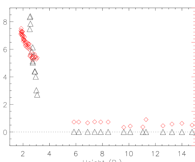
Figure 6: $\Delta\omega$ varied with leading edge height. The black triangles show the calculated result of $\Delta\omega$ at different altitudes. The red symbols show the CPA varied with the LEH of the CME as in Figure 2.

We applied Equation (1) to analyze the variation of $\Delta\omega$ during the 8 October 2007 CME’s propagation in the corona. The regions enclosed by the dotted – dashed line and the solid line in Figure 5 show the selected upper part and lower part in a 15^∘ angle range. The enclosed circle covers a 30^∘ angle range and corresponds to the mean angle width of this CME during its propagation in COR1-B FOV. Figure 6 shows the variation of $\Delta\omega$ and CPA with the CME’s leading edge heights. Shown as black triangles in Figure 6, the $\Delta\omega$ were positive for almost all heights. As we discussed above, this result means that an Equator – ward force was acting on the 8 October 2007 CME. This Equator – ward force could deflect the CME to a lower latitude. It is well consistent with the CPA observations shown as the red diamonds in Figure 6. During the CME’s outward propagation and its Equator – ward deflection, the value of $\Delta\omega$ decreased quickly. When the CME propagated to $\approx 5.5R_{\odot}$, $\Delta\omega$ almost reached the value of $\approx$0 and then stayed at $\approx$0. If $\Delta\omega$ equals zero, this means no obvious resultant force would act on the CME. Accordingly, it is quite natural that the CME propagated radially during this period, as the observations show. These results illustrate that the deflection of the CME was controlled by the background magnetic field and the gradient of magnetic energy density, which made the CME deflect to the region with lower magnetic energy density.

4 Summary and Discussion

We studied the kinematic evolution of the 8 October 2007 CME during its propagation in the corona. From the study of the CME’s propagation direction evolution in the meridian plane, we found that this CME obviously deflected to Equator at an early stage and then propagated almost radially. Combined with the three – dimension coronal magnetic field extrapolated from the CSSS model, we found that the CME deflected to the HCS at the beginning and then propagated almost along the HCS.

The velocity evolution of the CME during its propagation in the COR1-B FOV was also studied. The observations show that this CME underwent a two – phase evolution:

1. At the beginning, the CME propagated outward with a constant speed of $\approx$23. km.s^-1. This constant speed phase caused a velocity plateau in the velocity profile. Such a velocity plateau has also been reported and discussed by other authors [Dere et al., 1999; Srivastava et al., 1999; Zhang and Dere, 2006]. Dere et al. [1999] suggested that it might correspond to the period when the CME was opening the helmet streamer field lines.

2. After the velocity plateau, the speed of the 8 October 2007 CME continuously increased with an acceleration of 7.6$m.s^{-1}$.

These results show that this gradual CME experienced a multiphased acceleration. Srivastava et al. [1999] also found that in some cases of a gradual CME that they studied, a two – step speed profile occurred. They found that the CME accelerated initially until reaching a certain height and then moved with an almost constant speed for some time, before finally drifting away with the slow solar wind.

Furthermore, we performed a theoretical analysis to quantitatively study the CME’s deflection. We found that the deflection of the CME was controlled by the background magnetic field and that the CME tends to deflect to the region with lower magnetic energy density. We recall that we only consider the distribution of the magnetic energy at a given height, while the difference along the radial direction is neglected.

Figure 7: Distribution of the magnetic energy density of the Carrington rotation 1978 at the height of 3 $R_{\odot}$. The dashed line shows the neutral line.

In Section 3 we analyze the influence of the background magnetic field on the CME’s deflection from the point of view of the energy. From a different point of view, the electromagnetic force of the perturbed magnetic field acting on the CME consists of two components: the magnetic pressure force $f_{p}=\frac{\nabla B^{2}}{2\mu}$ and the magnetic tension force $f_{t}=\frac{\nabla\cdot BB}{\mu}$. The direction of the magnetic pressure force is from the higher magnetic field strength region to the lower magnetic field strength region. Besides, when a CME propagats outward, it compresses the background magnetic field lines as shown in Figure 4. In this situation, the magnetic tension force at a given point may be contrary to the compression direction. Because the magnitude of the tension force is related with the value of magnetic field strength, the resulting tension force that acts on the CME may also be directed toward the lower magnetic field strength region. Combined with the effect of magnetic pressure force and magnetic tension force, one can expect that a force directed toward the lower magnetic field strength region would act on the CME when it propagated outward and the CME tends to deflect to the lower magnetic energy density region.

Previous statistical results showed that the CME did deflect to the Equator at solar minimum, but no obvious regularity at solar maximum could be found [MacQueen, Hundhausen, and Conover, 1986; Cremades and Bothmer, 2004; Cremades, Bothmer, and Tripathi, 2006]. In the solar minimum the current sheet that corresponds to the lower magnetic energy density region is usually located near the Equator [e. g. Shodhan et al., 1994] similar to that we shown in Figure 5. Based on the result that the CME would deflected to the lower magnetic energy density region, the previous statistical results that the CME deflected to the Equator at solar minimum can be explained. The CME studied here happened on 8 October 2007, during the deep solar minimum of the 23rd cycle. It is a good example of the CME’s Equator – ward deflection in the solar minimum influenced by the background magnetic field. In the solar maximum, the distribution of the magnetic energy density was not as simple. Figure 7 shows an example of the magnetic energy density distribution at the height of 3 $R_{\odot}$ of the Carrington rotation 1978, which corresponds to the period from 03:13 UT 30 June 2001 to 08:08 UT 27 July 2001, during the solar maximum of the 23rd solar cycle. We found that the magnetic energy density distribution at solar maximum was complex and that no definite low magnetic energy density region where the CME would deflect to could be expected. Therefor, no obvious regularity of the deflection of a CME during solar maximum could be explained as the previous results showed.

The nonuniform distribution of the magnetic energy density may also exist in the longitude direction, as shown in Figure 5 and Figure 7. This nonuniform distribution was more obvious at solar maximum (shown in Figure 7). Thus, it could be expected that the CME would deflect to the east or west of the ecliptic plane because of the gradient of the magnetic energy density especially in solar maximum. This may provide another mechanism that could trigger the CME’s East – wWest deflection besides the interplanetary spiral magnetic field [Wang et al., 2004, 2006] and coronal holes [Gopalswamy et al., 2004, 2005, 2009]. The East – West deflections of the CME in ecliptic plane can influence the CME’s geoeffectiveness [Wang et al., 2006; Lugaz et al., 2010]. It was thought to be the cause of the East – West asymmetry distribution of earth – encountered CME’s source region [Wang, Wang, and Ye, 2002; Zhang et al., 2003].

Previous studies also suggested that the heliospheric magnetic field (HMF) would influence the CME and the shock’s propagation [Wei and Dryer, 1991; Smith, 2001; Yurchyshyn et al., 2007; Yurchyshyn, 2008; Xie et al., 2006]. By analyzing flare – associated shock wave events based on interplanetary scintillation (IPS) observation, Wei and Dryer [1991] found that all flare – associated shock waves tended to propagate toward the low latitude region near the solar Equator and the propagation directions tended toward the HCS. They suggested that this was caused by the dynamic action of near – Sun magnetic force on the ejected coronal plasma. Yurchyshyn [2008] found that the tilt of the coronal neutral line axis corresponded well with the magnetic cloud (MC) axis orientation observed at 1AU, but found no agreement with the EIT arcades. He suggested that the ejecta might be rotated in a way that it locally aligns itself with the heliopsheric current sheet. The HMF may have deflected the CME from its initial direction and, quite possible, rotated the axis of the CME as it moved through interplanetary space [Smith, 2001]. We showed here the whole process of the CME deflection to the HCS influenced by the heliospheric magnetic field and analyzed it for a very slow CME event. These results indicate that the heliospheric magnetic field could significantly influence the CME and its connected events.

We acknowledge the use of the data from STEREO/SECCHI. We thank Jie Zhang for helpful discussions. This work is supported by grants from the National Natural Science Foundation of China (40904046,40874075,40525014), the 973 National Basic Research Program (2011CB811403), Ministry of Education of China (200530), the Program for NewCentury Excellent Talents in University (NCET-08-0524), the Chinese Academy of Sciences (KZCX2-YW-QN511, KJCX2-YW-N28 and the startup fund) and the Fundamental Research Funds for the Central Universities.

References

- Burton et al. [1996] Burton, M.E., Smith, E.J., Balogh, A., Murphy, N.: 1996, In: Winterhalter, D., Gosling, J.T., Habbal, S.R., Kurth, W.S., Neugebauer, M. (eds.) AIP, CS-382, 506. doi:10.1063/1.51439.
- Cremades and Bothmer [2004] Cremades, H., Bothmer, V.: 2004, Astron. Astrophys. 422, 307. doi:10.1051/0004-6361:20035776.
- Cremades, Bothmer, and Tripathi [2006] Cremades, H., Bothmer, V., Tripathi, D.: 2006, Adv. Space Res. 38, 461. doi:10.1016/j.asr.2005.01.095.
- Dere et al. [1999] Dere, K.P., Brueckner, G.E., Howard, R.A., Michels, D.J., Delaboudinière, J.P.: 1999, Astrophys. J. 516, 465. doi:10.1086/307101.
- Gopalswamy et al. [2004] Gopalswamy, N., Yashiro, S., Krucker, S., Stenborg, G., Howard, R.A.: 2004, J. Geophys. Res. 109, A12105.
- Gopalswamy et al. [2005] Gopalswamy, N., Yashiro, S., Michalek, G., Xie, H., Lepping, R.P., Howard, R.A.: 2005, Geophys. Res. Lett. 32, L12S09.
- Gopalswamy et al. [2009] Gopalswamy, N., Mäkelä, P., Xie, H., Akiyama, S., Yashiro, S.: 2009, J. Geophys. Res. 114, A00A22.
- Howard et al. [2008] Howard, R.A., Moses, J.D., Vourlidas, A., Newmark, J.S., Socker, D.G., Plunkett, S.P., Korendyke, C.M., Cook, J.W., Hurley, A., Davila, J.M., Thompson, W.T., St Cyr, O.C., Mentzell, E., Mehalick, K., Lemen, J.R., Wuelser, J.P., Duncan, D.W., Tarbell, T.D., Wolfson, C.J., Moore, A., Harrison, R.A., Waltham, N.R., Lang, J., Davis, C.J., Eyles, C.J., Mapson-Menard, H., Simnett, G.M., Halain, J.P., Defise, J.M., Mazy, E., Rochus, P., Mercier, R., Ravet, M.F., Delmotte, F., Auchère, F., Delaboudinière, J.P., Bothmer, V., Deutsch, W., Wang, D., Rich, N., Cooper, S., Stephens, V., Maahs, G., Baugh, R., McMullin, D., Carter, T.: 2008, Space Sci. Rev. 136, 67. doi:10.1007/s11214-008-9341-4.
- Kaiser et al. [2007] Kaiser, M.L., Kucera, T.A., Davila, J.M., St. Cyr, O.C., Guhathakurta, M., Christian, E.: 2007, Space Sci. Rev., 198. doi:10.1007/s11214-007-9277-0.
- Kilpua et al. [2009] Kilpua, E.K.J., Pomoell, J., Vourlidas, A., Vainio, R., Luhmann, J., Li, Y., Schroeder, P., Galvin, A.B., Simunac, K.: 2009, Annales Geophysicae 27, 4491.
- Lugaz et al. [2010] Lugaz, N., Hernandez-Charpak, J.N., Roussev, I.I., Davis, C.J., Vourlidas, A., Davies, J.A.: 2010, Astophys. J. 715, 493.
- MacQueen, Hundhausen, and Conover [1986] MacQueen, R.M., Hundhausen, A.J., Conover, C.W.: 1986, J. Geophys. Res. 91, 31.
- Sheeley et al. [1997] Sheeley, N.R., Wang, Y.M., Hawler, S.H., Bruechner, G.E., Dere, K.P., Howard, R.A., Koomen, M.J., Korendyke, C.M., Michels, D.J., Paswaters, S.E., Socker, D.G., Cry, O.C.ST., Wang, D., Lamy, P.L., Llebaria, A., Schwenn, R.: 1997, Astrophys. J. 484, 472.
- Sheeley et al. [1999] Sheeley, N.R., Walters, J.H., Wang, Y.M., Howard, R.A.: 1999, J. Geophys. Res. 104, 24739. doi:10.1029/1999JA900308.
- Shen et al. [2007] Shen, C., Wang, Y., Ye, P., Zhao, X.P., Gui, B., Wang, S.: 2007, Astrophys. J. 670, 849. doi:10.1086/521716.
- Shodhan et al. [1994] Shodhan, S., Crooker, N.U., Hughes, W.J., Siscoe, G.L.: 1994, J. Geophys. Res. 99, 2531. doi:10.1029/93JA02909.
- Smith [2001] Smith, E.J.: 2001, J. Geophys. Res. 106, 15819.
- Srivastava et al. [1999] Srivastava, N., Schwenn, R., Inhester, B., Stenborg, G., Podlipnik, B.: 1999, Space Sci. Rev. 87, 303. doi:10.1023/A:1005189610536.
- Srivastava et al. [2000] Srivastava, N., Schwenn, R., Inhester, B., Martin, S.F., Hanaoka, Y.: 2000, Astrophys. J. 534, 468. doi:10.1086/308749.