FRII radio galaxies in the SDSS: Observational facts

Abstract

Starting from the Cambridge Catalogues of radio sources, we have created a sample of 401 FRII radio sources that have counterparts in the main galaxy sample of the 7th Data release of the Sloan Digital Sky Survey and analyse their radio and optical properties.

We find that the luminosity in the H$\alpha$ line – which we argue gives a better measure of the total emission-line flux than the widely used luminosity in [O iii] – is strongly correlated with the radio luminosity $P_{\rm 1.4GHz}$. We show that the absence of emission lines in about one third of our sample is likely due to a detection threshold and not to a lack of optical activity. We also find a very strong correlation between the values of $L_{{\rm H}\alpha}$ and $P_{\rm 1.4GHz}$ when scaled by $``M_{\rm BH}"$, an estimate of the black hole mass.

We find that the properties of FRII galaxies are mainly driven by the Eddington parameter $L_{{\rm H}\alpha}$/$``M_{\rm BH}"$ or, equivalently, $P_{\rm 1.4GHz}$/$``M_{\rm BH}"$. Radio galaxies with hot spots are found among the ones with the highest values of $P_{\rm 1.4GHz}$/$``M_{\rm BH}"$.

Compared to classical AGN hosts in the main galaxy sample of the SDSS, our FRII galaxies show a larger proportion of objects with very hard ionizing radiation field and large ionization parameter. A few objects are, on the contrary, ionized by a softer radiation field. Two of them have double-peaked emission lines and deserve more attention.

We find that the black hole masses and stellar masses in FRII galaxies are very closely related: $``M_{\rm BH}"$ $\propto$ $M_{*}^{1.13}$ with very little scatter. A comparison sample of line-less galaxies in the SDSS follows exactly the same relation, although the masses are, on average, smaller. This suggests that the FRII radio phenomenon occurs in normal elliptical galaxies, preferentially in the most massive ones. Although most FRII galaxies are old, some contain traces of young stellar populations. Such young populations are not seen in normal line-less galaxies, suggesting that the radio (and optical) activity in some FRII galaxies may be triggered by recent star formation. The $``M_{\rm BH}"$ – $M_{*}$ relation in a comparison sample of radio-quiet AGN hosts from the SDSS is very different, suggesting that galaxies which are still forming stars are also still building their central black holes.

Globally, our study indicates that, while radio and optical activity are strongly related in FRII galaxies, the features of the optical activity in FRIIs are distinct from those of the bulk of radio-quiet active galaxies.

An appendix gives the radio maps of our FRII galaxies, superimposed on the SDSS images, and the parameters derived for our analysis that were not publicly available.

1 Introduction

According to the Collins English Dictionary, the term ”radio galaxy” (RG) refers to a galaxy that is a strong emitter of radio waves. However, only sources powered by accretion onto a super massive black hole can produce the extended structures called radio jets and lobes, and we will use the term radio galaxy in reference only to those sources. Accretion unto a massive black hole is what is considered to be the energy source of active galactic nuclei (AGN). It manifests itself in different ways and with different strengths in the entire electromagnetic spectrum. Most active galactic nuclei in the Sloan Digital Sky Survey (SDSS, York et al. 2000) are not radio active. Conversely, not all classical radio galaxies with extended radio lobes have emission lines in their optical spectra (Hine & Longair, 1979), suggesting that optical and radio activity are not necessarily concommittent (Best et al. 2005b).

Radio galaxies can be divided into two classes according to the morphology of their radio structure (Fanaroff & Riley, 1974). FRI radio galaxies are core-dominated sources with radio jets fading and dissipating on a short distance from center, while FRII radio galaxies are edge-brightened sources with highly collimated jets. The sizes of both types of radio galaxies range from a few kiloparsecs for compact steep spectrum sources to a few megaparsecs for giant radio galaxies. FRII radio galaxies tend to be more luminous than FRI ones. Fanaroff & Riley suggested a dividing luminosity of $L_{178MHz}\sim$ 2.5 $\times$ 10²⁶W Hz^-1, but as shown by Ledlow & Owen (1996) the dividing luminosity between FRI and FRII radio sources is a function of the host galaxy optical luminosity.

With the availability of observational data from large radio and optical surveys came the possibility to examine the optical properties of large samples of radio galaxies. Best et al. (2005a) cross-identified radio sources from the NVSS (Condon et al. 1998) and FIRST (Becker et al. 1995) radio surveys with the main galaxy sample of the second data release of the SDSS (Abazajian et al. 2004). The resulting sample, which is not morphology-specific is likely dominated by FRI or compact radio-sources, as can be judged by the low radio luminosities of the vast majority of their sample.

Using this (or a similar) sample Kauffmann, Heckman & Best (2008) have argued that radio emission is likely due to the accretion of hot gas by massive black holes central to galaxies in a dense environment, while the optical AGN phenomenon, strongly favoured by the presence of a young stellar population, is likely due to the accretion of cold gas. However, their sample lacks the brightest radio sources, the FRII ones, both because they are rare in the local Universe and because the very extended angular sizes of these sources does not allow easy cross-identification with optical galaxies.

FRII radio galaxies constitute a much better defined class than FRI radio galaxies in terms of radio morphology (Fanaroff & Riley, 1974). Besides, because of the diversities of their optical properties, they constitute a prime target for understanding the relation between optical and radio activity.

We have assembled a sample of morphologically selected FRII galaxies with optical counterparts available in the SDSS. Here, we present the result of our study comparing the radio and optical properties of FRII radio galaxies, including giant radio galaxies, in order to get more insight into the activity phenomenon in galaxies. Our data sample is, by necessity, much smaller than the sample used by Kauffmann et al. (2008), since FRII galaxies are much less common than FRI galaxies at low redshifts. Due to the selection process (see next section), our sample does not allow us to tackle such issues as luminosity distribution functions, which are examined by Kauffmann & Heckman (2009) using the same sample as Kauffmann et al. (2008). But we can look for the presence of correlations that might improve our understanding of radio loud AGN.

The organization of the paper is as follows: In Section 2 we provide a brief description of the sample selection and data processing. In Section 3 we analyze the relation between the radio power of FRII sources and the strength of their optical activity. In Section 4 we focus on the special class of FRII galaxies that show hot spots. In Section 5 we discuss the emission line properties of FRII galaxies. In Section 6 we put FRII galaxies in the context of other groups of galaxies: line-less galaxies and radio-quiet AGN hosts. The main results of our investigation are summarized in Section 7.

Throughout this paper we assume a $\Lambda$ Cold Dark Matter cosmology with $H_{0}=71$km s^-1Mpc^-1, $\Omega_{\rm m}=0.27$, and $\Omega_{\Lambda}=0.73$ (Spergel et al. 2003).

2 The data

2.1 The sample

The main aim of our selection was to obtain a sample of FRII radio galaxies with a large range of radio powers and sizes in order to study the relation between their radio properties with the optical properties of their associated galaxies. Unfortunately, an automatic cross-correlation of radio and optical catalogues misses radio sources with large angular size, without radio core or with radio flux at the catalogue limit. On the other hand the luminosity profiles of radio structures are quite complex and the algorithms of automatic selection from radio maps are not sophisticated enough to recognize radio structures of different luminosity profiles. Thus the method used here is a combination of automatic and manual selection from catalogues and radio maps and we had to restrict ourselves to a tractable number of radio maps to examine.

For this purpose, we limited our search to radio sources present in the Cambridge Catalogues of Radio Sources: 3C (Edge et al. 1959; Bennett 1962), 4C (Pilkington & Scott 1965; Gower, Scott & Wills 1967), 5C (Pearson 1975; Pearson & Kus 1978; Benn et al. 1982; Benn & Kenderdine 1991; Benn 1995), 6C (Baldwin et al. 1985; Hales, Baldwin & Warner 1988; Hales et al. 1990, 1991, 1993; Hales, Baldwin & Warner 1993), 7C (Hales et al 2007), 8C (Rees 1990; Hales et al. 1995) and 9C (Waldram et al. 2003) and using the SDSS CrossID we crossidentified them with the sample of 926246 galaxies from the SDSS DR7 main galaxy sample (Abazajian 2009), keeping only those radio sources whose optical spectra are available in the SDSS. Taking into account the sometimes large positional uncertainties in the Cambridge Radio Catalogues we adopted 0.2 arcmin maximum distance between radio core and optical galaxy. Next, we excluded all objects classified in the SDSS as quasars. We postpone the study of the quasar sample of the SDSS DR7 (which also contains the Seyfert 1 galaxies) to a next paper. The Cambridge Radio Catalogues were based on radio maps made at different radio frequencies and with different resolution, thus morphological classification based on these maps would give incoherent results not easy to compare. Therefore, in a third step we inspected the NVSS and FIRST (if available) radio maps of all the remaining sources (almost 2000). These maps were made at the same frequency (1.4 GHz), but with different resolutions, what facilitates identification of the most common features in FRII radio galaxies which are extended radio lobes (NVSS), compact cores and hot spots (FIRST). Thereby we were able to remove FRI objects as well as sources with disturbed radio morphology or with angular size too small to determine the morphology (mostly sources with angular diameter $\theta$ $<$ 20 arcsec). In this step we also excluded misidentified sources.

The pre-selected sample contained only few sources with radio structures larger than 700 kpc, known as giant radio galaxies. However, there is a significant number of giant radio galaxies that can be included into our analysis. Therefore, we considered the known ones (using the lists of Janda 2006 and Machalski et al. 2007), and looked for their optical counterparts in the SDSS DR7 spectroscopic catalogue. This allowed us to include all the giant radio galaxies with available spectroscopic data into our final sample.

We thus obtained a sample of 401 FRII radio galaxies, out of which 23 have diameters larger than 700 kpc. Note that our sample is not complete in any sense and is not adequate to study luminosity functions. We used radio catalogues that were based on radio observations at different frequencies and made with different flux limits. But our sample does cover a wide range of radio powers and sizes.

The optical data (magnitudes and spectroscopy) come from the SDSS. The spectra were taken with 3 arcsec diameter fibers and cover a wavelength range of 3800–9200 Å with a mean spectral resolution of 1800. We use the data as given in the seventh data release.

Obviously, inferences derived from a given sample are not necessarily valid for another one. Many studies (e.g. Best. et al. 2005a,b; Kauffmann et al. 2008; Smolčić et al. 2009; Smolčić 2009) include different morphological types of radio galaxies without distinguishing among them. Those samples, however, go to much lower radio luminosities than ours, and are thus complementary in some respect. The Smolčić et al. (2009) sample is extracted from the VLA-COSMOS survey (Schinnerer et al. 2007), and has the advantage of the existence of many ancillary data at all wavelengths. Other samples (e.g. Rawlings et al. 1989, Zirbel & Baum 1995, Owen & Ledlow 1994), while focusing on FRII types or explicitly distinguishing them from FRI ones, have only limited information on the properties that can be derived from optical data, such as black hole masses or accurate emission line fluxes in the case of lines with small equivalent widths. The sample of Buttiglione et al. (2009, 2010) is extracted from the 3CR radio catalogue only, imposing a radio flux limit higher than ours. It distinguishes between FRII, FRI and so-called compact sources. The optical data come mostly from their own observations. But the analysis of the stellar continuum is not as advanced as ours (see Sect. 2.2), and parameters such as galaxy masses or black hole masses were not obtained. Thus our sample, although restricted to the Cambridge Catalogues of Radio Sources, is the only one that allows the exploration of the optical properties of FRII galaxies (including giants), comparing radio properties with galaxy masses or accretion rates on the central black hole. The redshifts in our sample range from 0.045 to 0.6.

2.2 Data processing

The 1.4 GHz radio luminosities, $P_{\rm 1.4GHz}$, of all the sources were calculated from the total flux density at this frequency obtained as a sum of fluxes of all components fitted to the each source and listed in the NVSS catalogue.

The angular sizes of the sources, defined as the distances between the hot spots or between the most distant bright structures in both lobes, as it is in the case of relic or FRI/II radio sources, were estimated manually either from the FIRST maps if available, or from the NVSS maps using the Aladin Sky Atlas. The manual method of deriving the angular size involves an error in this quantity of about 10%. The angular sizes were used to determine the linear (projected) diameters of the sources, $D$. In our sample, these extend from 15 kpc to 2080 kpc.

The optical parameters of the sample galaxies, i.e. their stellar masses and ages as well as the emission line fluxes are taken from the starlight database (Cid Fernandes et al. 2009). starlight (Cid Fernandes et al. 2005, see also Mateus et al. 2006) recovers the stellar population of a galaxy by fitting a pixel-by-pixel model to the spectral continuum (excluding narrow windows where emission lines are expected as well as bad pixels). The model is a linear combination of 150 simple stellar populations templates with ages 1 Myr $\leq t_{\star}\leq$ 18 Gyr, and metallicities $0.005\leq Z/Z_{\odot}\leq 2.5$. In this paper we use parameters that were calculated in the same way as in Cid Fernandes et al. (2010), i.e. using Bruzual & Charlot (2003) evolutionary stellar population models, with the STELIB library (Le Borgne et al. 2003), “Padova 1994” tracks (Bertelli et al. 1994) and Chabrier (2003) initial mass function. Emission lines fluxes are measured by Gaussian fitting in the residual spectra, which reduces the contamination by stellar absorption features. We checked, by visual inspection, all the SDSS spectra and corrected the line intensities in the very rare cases where the automatic procedures led to spurious results.

To correct the emission lines for extinction, one usually forces the observed H$\alpha$/H$\beta$ ratio to the theoretical case B recombination value of 2.9. Unfortunately, in our sample, there are many galaxies which do not have both H$\alpha$ and H$\beta$ fluxes measured with sufficient accuracy. In a preliminary step, we have computed the visual extinction, $A_{\rm V}$, using the Fitzpatrick (1999) extinction law parametrized with $R_{\rm V}$ =3.1 for all the objects in our sample having $S/N>3$ in both H$\alpha$ and H$\beta$. Figure 1 shows $P_{\rm 1.4GHz}$ vs $A_{\rm V}$. Objects for which $A_{\rm V}$ could not be evaluated are represented at an abscissa of 0. We see that there is no relation between the $A_{\rm V}$ and $P_{\rm 1.4GHz}$, in particular no indication of a tendency for $A_{\rm V}$ to increase with decreasing $P_{\rm 1.4GHz}$. It is therefore likely that the extinction is in fact between $\sim$ 0.5 and $\sim$ 1.2 for most of our galaxies for which we could not obtain it. Therefore, correcting the line intensities for extinction in some of the objects and not in others is not better justified than performing no extinction correction at all. In this paper we use only uncorrected line intensities (except in line ratio diagrams where the dereddening could be applied to all the objects in the plot).

Figure 1: The relation between the 1.4 GHz radio luminosity, $P_{\rm 1.4GHz}$, and $A_{\rm V}$ for our sample of FRII radio galaxies.

As mentioned above, the stellar masses used in this paper, $M_{*}$, were taken from the starlight database. They were obtained from the stellar masses corresponding to the light inside the fiber by correcting for aperture affect assuming that the mass-to-light ratio outside the fiber is the same as inside and scaling the fiber masses by the ratio between total (from the photometric data base) and fiber $z$-band luminosities. This correction is smaller than a factor of 2 in a large portion of our sample, but can amount to factors of up to 8. On the other hand, we do not correct the emission line luminosities for aperture effects, since the emission lines are expected to be emitted in the inner regions of the galaxies associated with the radio sources.

In this paper, we will often refer to the black hole masses of the galaxies, estimated from the observed stellar velocity dispersion given by the SDSS, $\sigma_{*}$, using the popular relation by Tremaine et al. (2002):

$${\rm log}M_{\rm BH}=8.13+4.02\,{\rm log}(\sigma_{*}/200\,{\rm km\,s^{-1}}).$$ (1)

The interpretation of such a formula is a challenge, since it seems to indicate a causal relation between the masses of two types of objects (galaxy bulges and black holes) that differ in size by 3–4 orders of magnitude. In particular, its range of validity is not clearly established. In the following, we will use the notation $``M_{\rm BH}"$ to refer to the “black hole mass” as derived from Eq. 1 to remember that it does not necessarily represent the true mass of the central black hole, but is merely an expression derived from the measured velocity dispersion.

We consider $M_{*}$ values only for objects with sufficiently good spectra (in practice we impose a S/N $>10$ in the continuum). The $``M_{\rm BH}"$ values will be considered only for those objects which, in addition, have $\sigma_{*}>60$ km s<sup>-1</sup>. In such a way, the values of $M_{*}$ and $``M_{\rm BH}"$ that we use will not be strongly affected by observational errors.

3 The relation between the radio power and optical activity of FRII sources

Figure 2: $L_{[\rm{O}\,\textsc{iii}]}$ versus $P_{\rm 1.4GHz}$, for FRII galaxies having $S/N>3$ in the [O iii] line. The straight line is the bissector regression line.

Rawlings et al. (1989) were the first to note the existence of an intrinsic correlation between the radio power and $L_{[\rm{O}\,\textsc{iii}]}$ in a sample of 39 FRII galaxies. They take it as evidence for a physical coupling of the processes that supply energy to the emission line region and to the extended radio source. Our sample confirms this trend and shows a very strong correlation, as seen in Fig. 2. The Pearson correlation coefficient is $R$=0.66 for a sample of 160 objects having the [O iii] line measured with a signal-to-noise ratio ($S/N$) larger than 3. Using the regression package of Akritas & Bershady (1996), the bissector regression line, assuming a typical error of 0.2 dex in all the observables, is found to be:

$${\rm log}L_{[\rm{O}\,\textsc{iii}]}=(1.37\pm 0.07)\times{\rm log}P_{\rm 1.4GHz}$$

$$+(-28.0\pm 1.7).$$ (2)

Note that, if $L_{[\rm{O}\,\textsc{iii}]}$ is taken to be a measure of the AGN luminosity in radio galaxies, one should in principle worry about the possible contribution of [H ii] regions. Kauffmann & Heckman (2009) have proposed a rough method to correct for this effect by taking into account the galaxy distance from the star forming branch in the BPT diagram. This, indeed should improve the estimate of the AGN luminosity of radio galaxies that experience star formation. In our sample of FRII galaxies, though, there is no star formation occuring presently, as argued later in this paper, therefore such a correction is not needed.

Figure 3: $L_{{\rm H}\alpha}$ versus $P_{\rm 1.4GHz}$, for FRII galaxies having $S/N>3$ in the H$\alpha$ line. The straight line is the bissector regression line.

The reason for using $L_{[\rm{O}\,\textsc{iii}]}$ as a way to estimate the total energy emitted in the lines is that [O iii] is often the strongest line in optical spectra. As a matter of fact, it is much better to use the luminosity of H$\alpha$, $L_{{\rm H}\alpha}$. Even if H$\alpha$ may be weaker than [O iii], the fact that its intensity is proportional to Ly$\alpha$, which is 8 times stronger, makes of it a far more reliable indicator of the total energy emitted in the lines. Of course, the bolometric correction factor will not be the same for $L_{[\rm{O}\,\textsc{iii}]}$ and $L_{{\rm H}\alpha}$. A further argument for preferring $L_{{\rm H}\alpha}$ to $L_{[\rm{O}\,\textsc{iii}]}$ is that its value is independent of the ionization state, contrary to $L_{[\rm{O}\,\textsc{iii}]}$. Fig. 3, shows $L_{{\rm H}\alpha}$ as a function of $P_{\rm 1.4GHz}$, for the 145 FRII galaxies having $S/N>3$ in the H$\alpha$ line. As expected, the correlation is better: $R$=0.72. The bissector regression line is:

$${\rm log}L_{{\rm H}\alpha}=(1.13\pm 0.07)\times{\rm log}P_{\rm 1.4GHz}+$$

$$(-21.9\pm 1.8).$$ (3)

Thus, both $L_{[\rm{O}\,\textsc{iii}]}$ and $L_{{\rm H}\alpha}$ (when available) indicate a strong correlation between AGN activity and radio power of these extended radio sources. While qualitatively, this result is in agreement with the one found by Zirbel & Baum (1995) who used H$\alpha$+ [N ii], there is a significant difference. Zirbel & Baum (1995) found that, for the FRII radio galaxies they considered, the exponent of the relation between $L_{{\rm H}\alpha+[\rm{N}\,\textsc{ii}]}$ and radio power is $0.75\pm 0.09$, while we find that the exponent of the relation between $L_{{\rm H}\alpha}$ and radio power is as large as $1.13\pm 0.07$. We checked that this difference is not due to the [N ii] line, whose contribution might a priori change systematically with luminosity. As a matter of fact, it seems that the difference is mainly due to the way the regression line is obtained.

Buttiglione et al. (2010) found that high excitation radio galaxies (HEGs) follow a slightly different $L_{[\rm{O}\,\textsc{iii}]}$ vs $P_{\rm 1.4GHz}$ relation than low excitation radio galaxies (LEGs). We believe that this is simply the consequence of the fact that $L_{[\rm{O}\,\textsc{iii}]}$ is strongly dependent of the ionization state and is therefore a biased estimator of the total AGN energy emitted in the lines. Note that $L_{{\rm H}\alpha}$, in addition to being a good estimator of the energy emitted in the lines, is also an exact estimator of the total number of ionizing photons emitted by the AGN (if all of them are absorbed by the gas).

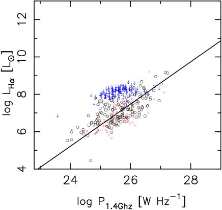
Figure 4: $L_{{\rm H}\alpha}$ versus $P_{\rm 1.4GHz}$ for FRII galaxies of our sample. Black circles correspond to objects having $S/N>3$ in the H$\alpha$ line, small (red in the electronic version) circles to objects where the H$\alpha$ line is detected with a lower S/N. The grey (blue in the electronic version) arrows correspond to objects where H$\alpha$ is not detected although not redshifted out of the SDSS wavelength range, and represents the lower limit in H$\alpha$ flux that could be detected given the S/N of the spectrum in the continuum. The straight line is the same as in Fig. 3.

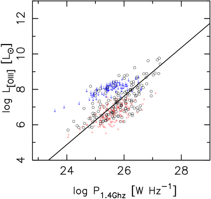
Figure 5: $L_{[\rm{O}\,\textsc{iii}]}$ versus $P_{\rm 1.4GHz}$ for FRII galaxies of our sample. The presentation is analogous to that in Fig. 4. The straight line is the same as in Fig. 2.

Figures 2 and 3 were constructed by using only data for which the relevant emission lines have a S/N $>3$. However, even including data with much worse S/N, as shown in Fig. 4 with small (red in the electronic version) circles points for the case of $L_{{\rm H}\alpha}$, the regression lines remain the same and the dispersion is not increased. This is because the correlation is so strong over a range of several decades in optical and radio luminosities while the measurement of a line intensity cannot be wrong by a factor more than $\sim$ 2 when it is detected, which is negligible with respect to the range of luminosities encountered.

The fact that such a strong correlation exists for the 298 FRII galaxies with the [O iii] line detected and the 205 ones with the H$\alpha$ line detected, in a total sample of 401 radio galaxies (of which 45 have redshifts larger than 0.4, which shifts the H$\alpha$ line out of the SDSS wavelength range) raises the question of whether this is a universal relation for FRII galaxies. Using the S/N ratio in the continuum of the objects where those lines have not been detected and assuming a typical emission-line width of 10Å, we have estimated the minimum detectable flux in these lines for each object. These numbers, converted into luminosities, are plotted as grey (blue in the electronic version) arrows in Fig. 4. One can see that the objects with undetected lines in H$\alpha$ could well follow exactly the same trend as the ones with detected H$\alpha$. A similar figure for [O iii] (Figure 5) gives the same result. Note that this is at variance with the finding by Buttiglione et al. (2010) that, in their sample (which however does not contain only FRII galaxies), for objects with undetected [O iii] the upper limits on [O iii] luminosities are well below the prediction of the correlation between emission line and radio power. Thus, we find no evidence for the existence of line-less FRII radio galaxies.

Figure 6: The relation between $L_{{\rm H}\alpha}$/$``M_{\rm BH}"$ and $P_{\rm 1.4GHz}$/$``M_{\rm BH}"$ for FRII galaxies having $S/N>3$ in the H$\alpha$ line. The straight line is the bissector regression line.

In their sample of radio galaxies (of all types), Kauffmann et al. (2008) did not find a strong correlation between $L_{[\rm{O}\,\textsc{iii}]}$ or$L_{{\rm H}\alpha}$ and $P_{\rm 1.4GHz}$, but when scaling the emission-line and radio luminosities by the black hole mass, they do find some correlation between normalized radio power and accretion rate.

In Fig. 6, we show $L_{{\rm H}\alpha}$/$``M_{\rm BH}"$ vs $P_{\rm 1.4GHz}$./$``M_{\rm BH}"$ for our sample of FRII radio galaxies having $S/N>3$ in the H$\alpha$ line. The correlation coefficient is $R$=0.77. To our knowledge, this is the first time that such a strong correlation is shown to exist between $L_{{\rm H}\alpha}$/$``M_{\rm BH}"$ and $P_{\rm 1.4GHz}$./$``M_{\rm BH}"$ in powerful radio galaxies. The bissector regression line is:

$${\rm log}L_{{\rm H}\alpha}/``M_{\rm BH}"=(1.19\pm 0.07)\times{\rm log}P_{\rm 1.4GHz}/``M_{\rm BH}"+$$

$$(-21.8\pm 1.3).$$ (4)

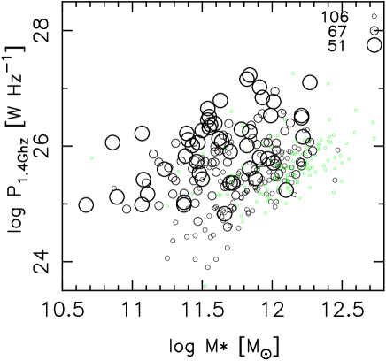
Figure 7: The relation between: $P_{\rm 1.4GHz}$ and the stellar masses $M_{*}$ of the FRII galaxies. The symbol sizes correspond to values of the “Eddington parameter” $L_{{\rm H}\alpha}$/$``M_{\rm BH}"$. Large circles: log $L_{{\rm H}\alpha}$/$``M_{\rm BH}"$ $>-0.8$ ; intermediate size circles: log $L_{{\rm H}\alpha}$/$``M_{\rm BH}"$ between $-1.5$ and $-0.8$; small black circles: log $L_{{\rm H}\alpha}$/$``M_{\rm BH}"$ $<-1.5$; very small grey (green in the electronic version) circles: H$\alpha$ not detected.

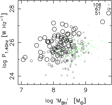
Figure 8: The relation between: $P_{\rm 1.4GHz}$ and $``M_{\rm BH}"$ for the FRII galaxies. Same symbols as in Fig. 7.

In Fig. 7 we investigate how the value of the ratio $L_{{\rm H}\alpha}/``M_{\rm BH}"$ (from now on referred to as the Eddington parameter, by similarity with Kauffmann & Heckman 2009) is distributed in the ($P_{\rm 1.4GHz}$, $M_{*}$) plane. The sizes of the black circles correspond to the value of $L_{{\rm H}\alpha}/``M_{\rm BH}"$, as indicated in the figure caption. The small grey (green in the electronic version) circles represent objects for which H$\alpha$ is not observed. Roughly, the circle sizes decrease perpendicularly to the weak trend between $P_{\rm 1.4GHz}$ and $M_{*}$ (the Pearson correlation coefficient between $P_{\rm 1.4GHz}$ and $M_{*}$ is $R$=0.31). This means that the most powerful radio galaxies are also the ones with the largest Eddington parameter, for a given galaxy mass, and that, for a given radio power, the Eddington parameter increases as the galaxy mass decreases. Note that the lower envelope of the points in this diagram increases with increasing $M_{*}$. This is a transcription, in the ($P_{\rm 1.4GHz}$, $M_{*}$) plane, of the fact that the FRII/FRI transition occurs in a narrow zone of the radio luminosity - optical luminosity diagram as shown by Owen & Ledlow (1994).

In the ($P_{\rm 1.4GHz}$,$``M_{\rm BH}"$) plane, as seen in Fig. 8, the distribution of $L_{{\rm H}\alpha}/``M_{\rm BH}"$ with respect to the axes is similar to that seen in Fig. 7, i.e. perpendicular to the first diagonal (as implied by the strong correlation between $P_{\rm 1.4GHz}$ and $L_{{\rm H}\alpha}$). But the radio power and $``M_{\rm BH}"$ are only loosely correlated ($R$=0.15).

4 Properties of FRII radio sources with hot spots

Fanaroff & Riley (1974) used the ratio of the distance between the brightest regions in lobes placed on opposite sides of a central galaxy to the total source size as a criterion to classify extended radio sources. The regions of the highest brightness at the end of lobes are places where the relativistic jets emanating from active galactic nuclei interact with the environment, and are called hot spots (the detailed definition of hot spots can be found in Hardcastle et al., 1998). Not all radio sources show hot spots. For example, in the case of radio relicts, i.e. sources where the central activity has already stopped, hot spots are not present (Kaiser et al. 2000, Marecki & Swoboda, 2011). One can thus expect that the presence of hot spots is related with some properties of the AGN and its environment.

We have searched our sample of FRII radio sources for the presence of hot spots. We were able to do this only for sources with available FIRST radio maps (whose resolution is much better than that of NVSS maps) and with angular size large enough to separate the bright, compact components from the bright lobes. Of 211 sources with suitable radio maps and large enough angular sizes, 51 were found to have prominent hot spots.

Owen and Laing (1989) proposed an alternative way of classifying radio sources in terms of morphology. They introduced 3 classes of radio sources: Twin Jet, Classical Double and Fat Double sources. Twin Jet galaxies fit into the FRI type, Classical Doubles are galaxies with compact hot spots and elongated lobes and fit into the FRII class. Fat Double galaxies with diffuse lobes and bright outer rims can be included into FRII or FRI/II classes. Our FRII radio galaxies with hot spots are thus genuine Classical Doubles. Owen and Laing showed, in their Fig. 6, that Classical Double sources are more luminous in radio but less luminous in the optical than Twin Jet and Fat Double radio galaxies.

We show, in Fig. 9, how radio galaxies with and without hot spots are located in the $P_{\rm 1.4GHz}$ vs $M_{*}$ diagram. Sources with prominent hot spots are represented by stars. Sources which definitely do not show any hot spot are represented by big dots. Sources for which we could not do the classification are represented by small dots. As can be seen in the figure, for a given $M_{*}$ the radio luminosities of FRII radio galaxies with hot spots are systematically higher than those of most of the remaining galaxies. It can also be seen that the luminosities of sources with hot spots increase with increasing $M_{*}$. This suggests that the presence of hot spots is not simply related to a high $P_{\rm 1.4GHz}$. In Fig. 10 we show the same sources in the $P_{\rm 1.4GHz}$/$``M_{\rm BH}"$ vs $M_{*}$ diagram. Here, the separation between the two groups of FRII galaxies is even more pronounced and one can see that sources with hot spots have larger $P_{\rm 1.4GHz}$/$``M_{\rm BH}"$. In other words, hot spot prominence is connected to higher radio efficiency (and, consequently, a higher Eddington parameter).

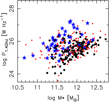
Figure 9: The distribution of the FRII radio sources with hot spots in the ($P_{\rm 1.4GHz}$, $M_{*}$) plane. Stars: sources with hot spots; Big dots: sources without hot spots. Small dots: Sources for which the classification could not be made.

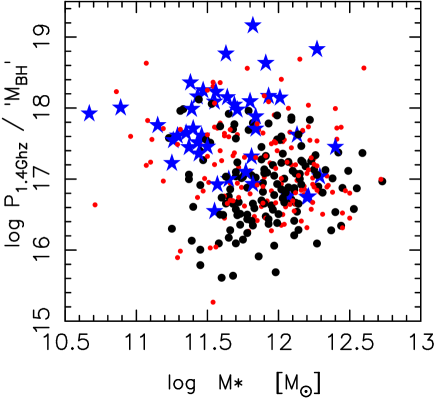
Figure 10: The distribution of the FRII radio sources with hot spots in the ($P_{\rm 1.4GHz}$/$``M_{\rm BH}"$, $M_{*}$) plane. The symbols are the same as in Fig. 9.

5 Emission line analysis

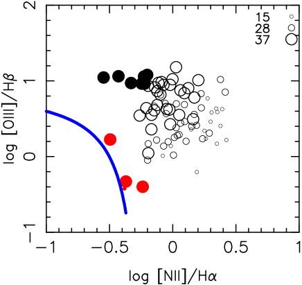
Figure 11: FRII radio galaxies in the BPT diagram for objects having S/N $>3$ in all the relevant lines. The sizes of the symbols correspond to the Eddington parameters $L_{{\rm H}\alpha}$/$``M_{\rm BH}"$ like in Fig. 8. A few objects are represented in filled black or grey (red in the electronic version) circles. They are discussed in the text. The thick grey (blue in the electronic version) curve represents the line above which all the galaxies are believed to host an AGN, according to S06.

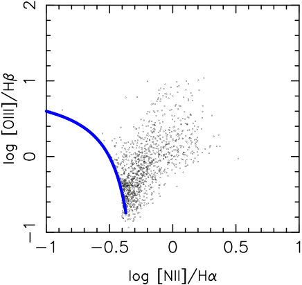
Figure 12: The BPT diagram for a comparison sample of 1000 galaxies. These galaxies are randomly drawn from SDSS DR7 galaxies that lie above the S06 line with S/N $>3$ in all the relevant lines. The thick grey (blue in the electronic version) curve represents the S06 line.

We now investigate in more detail the emission lines in FRII radio galaxies, and in particular the line ratios, in order to get more clues about the characteristics of nuclear activity in these objects.

5.1 Diagnostic diagrams

Figure 11 plots our FRII radio galaxies in the classical Baldwin, Phillips & Terlevich (1981, BPT) diagram, used to characterize the ionizing source of the gas in galaxies. We have plotted only the sources with S/N $>3$ in all the relevant lines, which limits our original sample of FRII galaxies to only 81 objects. The sizes of the circles correspond to the values of $L_{{\rm H}\alpha}$/$``M_{\rm BH}"$ like in Fig. 8. The galaxies represented with the filled black and grey (red in the electronic version) circles will be discussed in more detail later. The thick grey (blue in the electronic version) curve represents the line above which all the galaxies are believed to host an AGN, according to Stasińska et al. (2006, S06). One can see that all our FRII galaxies lie above the S06 line, as expected. Their distribution in the BPT plane is however very different from that of a random comparison sample of 1000 SDSS DR7 galaxies that lie above the S06 line and have S/N $>3$ in all the relevant lines, as seen in Fig. 12. Most of the objects in the comparison sample gather close to the blue line. In those, star formation is believed to compete with the AGN to produce the emission lines, with the contribution of star formation decreasing away from the blue line (S06). In our FRII sample, there are only a few objects (represented in grey (red in the electronic version) in Fig. 11) which lie close to the blue line. Most of the FRII galaxies lie well away from it, indicating that the line emission in them is entirely (or almost entirely) due to their AGN. One can also see that in our FRII sample, there is a much larger proportion of objects having high [O iii]/H$\beta$ and low [N ii]/H$\alpha$ (those represented in black in Fig. 11) than in the comparison sample.

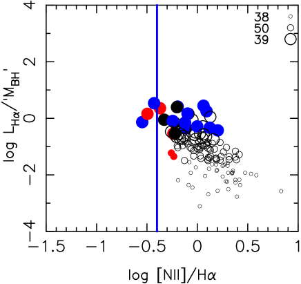
Figure 13: FRII radio galaxies in the $L_{{\rm H}\alpha}$/$``M_{\rm BH}"$ vs [N ii]/H$\alpha$ diagram. Only objects with S/N $>10$ in the continuum and $>3$in [N ii] and H$\alpha$ are shown. Symbols are like in Fig. 8, but some of the large open circles have been replaced by filled blue circles (discussed in the text). The vertical line corresponds to log [N ii]/H$\alpha$ $=-0.4$ (see S06).

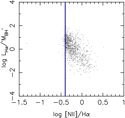
Figure 14: The same comparison sample as in 3 in the $L_{{\rm H}\alpha}$/$``M_{\rm BH}"$ vs [N ii]/H$\alpha$ diagram. Only objects with S/N $>10$ in the continuum are shown. The vertical line corresponds to log [N ii]/H$\alpha$ $=-0.4$.

Figure 13 plots our FRII radio galaxies in the $L_{{\rm H}\alpha}$/$``M_{\rm BH}"$ vs [N ii]/H$\alpha$ diagram, which allows one to accomodate 127 of our objects (they must have S/N $>10$ in the continuum and $>3$ in [N ii] and H$\alpha$), in comparison with the 81 in the BPT diagram. The vertical line has been proposed by Stasińska et al. (2006) to separate galaxies containing an AGN in a more “economical” way than the BPT diagram. Some of the grey (red in the electronic version) and black filled circles actually lie to the left of the vertical line, paradoxically in the region were only “pure star-forming galaxies” should lie. We will come back to this below. Figure 14 plots our comparison sample in the same diagram, still restricting to galaxies with S/N $>10$ in the continuum. Again, the distribution of the comparison sample in this diagram is significantly different from that of our FRII sample. Most of our FRII galaxies, even in this diagram which includes more points th an the BPT diagram, still lie far away from the star-forming region. The bulk of the galaxies from the comparison sample, which lie close to the log [N ii]/H$\alpha$ $=-0.4$ line, have higher values of $L_{{\rm H}\alpha}$/$``M_{\rm BH}"$. This is because, in the latter objects, $L_{{\rm H}\alpha}$ is affected by photoionization by recently born massive stars.

5.2 Special cases

We now turn to discuss the special cases, represented by filled black and grey (red in the electronic version) circles in Figs. 11 and 13.

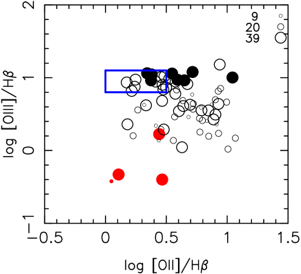
Figure 15: FRII radio galaxies in the [O iii]/H$\beta$ vs [O ii]/H$\beta$  diagram for objects having S/N $>3$ in all the relevant lines. The sizes of the symbols correspond to the “Eddington parameters” $L_{{\rm H}\alpha}$/$``M_{\rm BH}"$ like in Fig. 8. The objects represented in filled black or grey (red in the electronic version) circles are the same as in Figs. 11 and Fig. 13. The box delimits a zone with log [O iii]/H$\beta$ $>0.8$ and log [O ii]/H$\beta$ $>-0.5$, to be compared to Fig. 16.

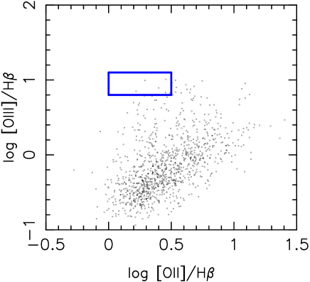
Figure 16: The [O iii]/H$\beta$ vs [O ii]/H$\beta$  diagram for the comparison sample. The zone delimited by the box is the same as in Fig. 15.

In the BPT diagram, the position of galaxies containing an AGN is determined by the hardness of the ionizing radiation field, the ionization parameter (which scales like the surface density of ionizing photons per atom of emitting gas) and the O/H and N/O ratios. The distance to the blue curve in Fig. 11 increases with hardness of the radiation field, while an increase of the ionization parameter moves the points “parallel” to the curve towards higher values of [O iii]/H$\beta$.

The objects represented by black circles in Fig. 11 are thus likely to be characterized by an exceptionally hard radiation field and a large ionization parameter as compared to the bulk of optical AGN. However it is possible that their position to the left of most galaxies could be due to a small N/O ratio rather than to a large ionization parameter. Figure 15 shows our FRII radio galaxies in the [O iii]/H$\beta$ vs [O ii]/H$\beta$  diagram. This diagram is not so efficient as the BPT diagram in distinguishing star forming galaxies from galaxies hosting an AGN, as shown by S06, and therefore is less popular. But if one knows that one is dealing with AGN galaxies, as is the case here, this diagram is very useful, since it does not depend on the N/O ratio which spans a large range of values in massive galaxies. The points represented in black in Fig. 15 are the same as those represented in black in Figs. 11 and 13. One can therefore infer that many of them have actually a small N/O ratio. On the other hand, the objects that, schematically, are found in the box in Fig. 15 certainly have both a very hard ionizing radiation field and a high ionization parameter. There are 13 such objects out of 69 objects appearing in Fig. 15, while there are only 8 objects out of nearly 1000 in the box in Fig. 16 constructed with the comparison sample. Thus, the sample of FRII radio galaxies is characterized by a large proportion of AGNs with the hardest ionizing radiation field and highest ionization parameters. The objects that appear in the blue box in Fig. 15 are represented with filled grey (blue in the electronic version) circles in Fig. 13 (unless they were already black). Fig. 13 thus shows that the objects with the highest ionization parameters also belong to the ones with the largers values of the Eddington parameter, $L_{{\rm H}\alpha}$/$``M_{\rm BH}"$.

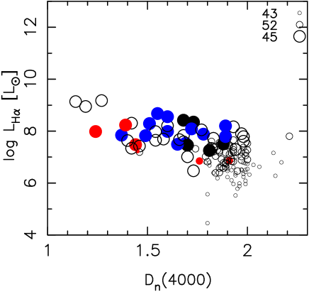
Figure 17: FRII radio galaxies in the $L_{{\rm H}\alpha}$ vs $D_{\rm n}(4000)$ plane. Only objects with S/N $>10$ in the continuum are shown. The symbols are exactly the same as in Fig. 11.

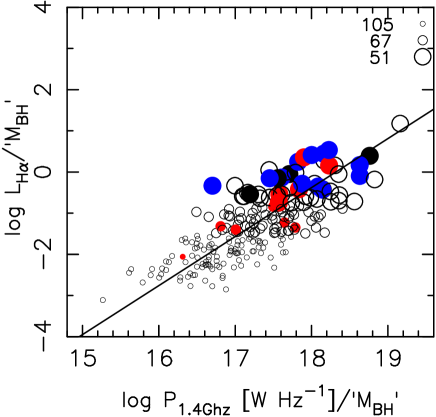
Figure 18: FRII radio galaxies in the $L_{{\rm H}\alpha}$/$``M_{\rm BH}"$ vs $P_{\rm 1.4GHz}/``M_{\rm BH}"$ plane. Only objects with S/N $>10$ in the continuum are shown. The symbols are exactly the same as in Fig. 13.

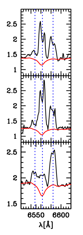
Figure 19: Spectra of the objects with double lines in the H$\alpha$ and [N ii] region. Top: object 0818.52395.570, one of the grey (red in the electronic version) points in Fig. 11. Middle: object 0902.52409.325, one of the grey (red in the electronic version) points in Fig. 11. Bottom: object 0932.52620.071, the third of our FRII galaxies with possible double lines.

The nature of the objects represented by grey (red in the electronic version) circles in Figs. 11, 13 and 15 is more difficult to understand. Those objects are close to the blue curve in the BPT diagram, so one could think they belong to the class of so-called composite galaxies, where the ionization by young massive stars competes with that of the AGN. If this is the case, one would expect the break at 4000Å, $D_{\rm n}(4000)$, to have a low value, of the order of 1–1.5, indicating the presence of young stellar populations (Bruzual 1983; Cid Fernandes et al. 2005). Figure 17 shows the positions of those galaxies with respect to the other ones from our FRII sample in the $L_{{\rm H}\alpha}$ vs $D_{\rm n}(4000)$ plane. Here, we use the definition of Balogh et al. (1999) for $D_{\rm n}(4000)$ and consider only spectra with a S/N $>10$ in the continuum. It can be seen that, indeed, those objects are among the ones with the youngest stellar populations.

Since, in the BPT diagram, and also in the [O iii]/H$\beta$ vs [O ii]/H$\beta$ diagram, the objects lie so much to the left of the remaining ones, the contribution of massive star ionization should be by far dominant. Following the composite photoionization models by S06 the contribution of the AGN to H$\alpha$ should be of only 3%. In such a case, those objects should stand out from the relation between $L_{{\rm H}\alpha}$/$``M_{\rm BH}"$ and $P_{\rm 1.4GHz}/``M_{\rm BH}"$. We show again the $L_{{\rm H}\alpha}$/$``M_{\rm BH}"$ vs $P_{\rm 1.4GHz}/``M_{\rm BH}"$ plot for our FRII radio galaxies, this time using the same symbols as in Fig. 13. We see that, although the grey (red in the electronic version) points are found above the mean of the $L_{{\rm H}\alpha}$/$``M_{\rm BH}"$ vs $P_{\rm 1.4GHz}/``M_{\rm BH}"$ relation, they do not stand out particularly with respect to the remaining objects. Therefore, we are inclined to think that the location of the grey (red in the electronic version) points in the emission-line diagnostic diagrams, rather than being due to an overwhelming presence of young stars, should be attributed to a much softer ionizing radiation as compared with the rest of the AGNs.

There is another intriguing characteristc of those objects. Two of them, 0818.52395.570 and 0902.52409.325 seem to have double line profiles, as can be seen in Fig. 19. There is only one other object with such profiles in our sample of FRII galaxies, also shown in Fig. 19. According to Liu et al. (2010a and b), such features are likely due to massive binary black holes. Clearly, those objects deserve further, more detailed observations, to uncover their real nature.

6 FRII galaxies in perspective

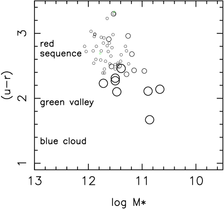
Figure 20: The rest-frame (u-r) color as a function of $M_{*}$ for the FRII galaxies with $z<0.1$. The symbol sizes represent correspond to the values of log $L_{{\rm H}\alpha}$/$``M_{\rm BH}"$, as in Fig. 7.

Figure 21: The rest-frame (u-r) color as a function of $M_{*}$ for a random comparison sample of 2000 objects in the SDSS with with $z<0.1$.

Figure 22: $``M_{\rm BH}"$ vs $M_{*}$ (left) and $M_{*}$ vs $D_{\rm n}(4000)$ (right) for our sample of FRII galaxies. The straight line is the bissector regression line given by Eq. 5.

Figure 23: The same as Fig. 22 but for a random sample of 1000 line-less galaxies in the SDSS. The straight line is the same as in Fig. 22.

Figure 24: $``M_{\rm BH}"$ vs $M_{*}$ (left) and $``M_{\rm BH}"$/$M_{*}^{1.13}$ vs $D_{\rm n}(4000)$ (right) for a random sample of 1000 galaxies considered to contain an AGN (i.e. galaxies that lie above the S06 curve in the BPT diagram). The straight line is the same as in Fig. 22.

We now characterize our population of FRII radio galaxies with respect to populations of related objects analyzed with the same procedures.

In Fig. 20 we show the position of our FRII galaxies in the classical color-mass, (u-r) vs $M_{*}$, diagram. Only the 57 objects with redhifts $z<1$ are shown, for a sound comparison with Fig. 4 of Smolčić (2009). This, of course, suppresses the most luminous and massive of our FRII radio galaxies, as can be seen when comparing Fig. 20 with Fig. 7. Still, the objects from our FRII sample that remain in Fig. 20 tend to have higher masses than those appearing in Fig. 4 of Smolčić (2009), due to the fact that the latter is based on a sample likely dominated by galaxies associated to compact or FRI radio sources. For comparison, in Fig. 21 we plot a random sample of 2000 galaxies of all types from the SDSS (again with redshifts $z<1$). In both Figs. 20 and 21, we indicate the approximate colour of the red sequence, green valley and blue cloud, following the nomenclature of Bell et al. (2004). In Fig. 20 the symbol sizes represent the values of $L_{{\rm H}\alpha}$/$``M_{\rm BH}"$, like in Fig. 7. We can see that the FRII galaxies with lowest Eddington parameters fall in the region of the red sequence, while those with the largest Eddington parameters fall in the region of the green valley. This reminds the result of Smolčić (2009) for low- and high-excitation AGNs of various radio morphologies. This does not mean, however, that high-excitation (or high $L_{{\rm H}\alpha}$/$``M_{\rm BH}"$) radio galaxies are not intrinsically red. As a matter of fact, the spectra of most of our FRII galaxies, including most of those with high Eddington parameters, have features similar to those of red galaxies. Simply, the effect of the active nucleus is to bias the photometric colour of the host galaxy, as shown for example by Pierce et al. (2010).

In Fig. 22 we represent our FRII sample in the $``M_{\rm BH}"$ vs $M_{*}$ plot (left) and in the $M_{*}$ vs $D_{\rm n}(4000)$ plot (right).

Figure 23 shows the same, but for a random sample of 1000 line-less galaxies in the SDSS (S/N $<2$ in all major emission lines). Those galaxies are typical red galaxies that show no sign of activity.

The correlation between $``M_{\rm BH}"$ and $M_{*}$ for FRII galaxies is very strong ($R$=0.70). The bissector regression line, assuming errors of 0.2 dex on each quantity, is given by:

$${\rm log}``M_{\rm BH}"=(1.13\pm 0.058)\times{\rm log}M_{*}-$$

$$(4.97\pm 0.69).$$ (5)

It is plotted in Fig. 22, as well as in Fig. 23, for reference. Clearly, this line is also a good fit to the relation observed between $``M_{\rm BH}"$ and stellar mass in line-less galaxies. Here, the correlation coefficient is even as large as $R$=0.85. We may note that the slope of the log $``M_{\rm BH}"$ – log $M_{*}$ relation is slightly, but significantly, smaller than one. One can notice, also, that the distribution of stellar masses and “black hole masses” are not exactly the same in the two samples: they are shifted towards higher values in the FRII sample. This implies that the FRII phenomenon does not occur in less massive line-less galaxies.

In the $M_{*}$ vs $D_{\rm n}(4000)$ diagram, although most FRII galaxies are old, as indicated by the $D_{\rm n}(4000)$ index already commented before, there are a few galaxies which have $D_{\rm n}(4000)$ $<$ 1.5, indicating the presence of young stellar populations (with ages of the order of $10^{7}-10^{8}$ yr). There is no hint of such populations in the comparison sample of line-less galaxies, as seen in Fig. 23. Note that, in the FRII sample, young stellar populations can occur at any value of $M_{*}$. This suggests that there is a connection between this recent star formation, presumably due to a collision, and the optical and radio activity.

If we now compare Fig. 22 (left) with Fig. 24 (left), which is identical to Fig. 23 (left) but for our comparison sample of galaxies that lie above the blue curve in the BPT diagram (Fig. 11), we see that $``M_{\rm BH}"$ and $M_{*}$ are not so well correlated as in the previous sample. In this case, we are mostly dealing with spiral galaxies, where the bulge is not very prominent, so the estimate of the black hole mass using the measured stellar velocity dispersion might be biased. However, when excluding galaxies with redshift $>0.1$, so that the measurement of $\sigma_{*}$ is not strongly affected by the galaxy disk, we obtain the same picture. The bulk of objects deviate from the $``M_{\rm BH}"$ – $M_{*}$ relation obtained for FRII or line-less galaxies. For a given galaxy mass, $``M_{\rm BH}"$ tends to be smaller. This suggests that those galaxies, which are still forming stars, are also still building their central massive black hole. To test this suggestion, we plot, in Fig. 24 (right), the values of $``M_{\rm BH}"$/$M_{*}^{1.13}$ (which is constant in the more evolved, line-less galaxies of Fig. 23 as a function of $D_{\rm n}(4000)$ for the same sample as in in Fig. 24 (left). We clearly see a that younger, i.e. less evolved galaxies that have smaller $D_{\rm n}(4000)$ tend to have smaller $``M_{\rm BH}"$/$M_{*}^{1.13}$ , and that this ratio increases with $D_{\rm n}(4000)$.

7 Summary

Using the Cambridge Catalogues of radio sources we have built a sample of FRII radio galaxies whose spectra are available in the main galaxy sample of SDSS DR7. From this sample, after inspection of the NVSS and FIRST radio maps, we extracted a sample of 401 FRII radio galaxies. In this paper, we examined the optical and radio properties of those objects, in order to find new clues about the relation between radio activity and the optical manifestations of the AGN in those objects. The stellar masses, emission line equivalent widths and fluxes were taken from the starlight database (Cid Fernandes et al. 2009).

We found that the luminosity in the H$\alpha$ line – which we argue gives a better measure of the total flux in the emission lines than the widely used luminosity in [O iii] – is strongly correlated with the radio luminosity $P_{\rm 1.4GHz}$ over more than three orders of magnitude in $P_{\rm 1.4GHz}$. A similar result was found by Zirbel & Baum (1995), using H$\alpha$ + [N ii], but they obtained $L_{{\rm H}\alpha+[\rm{N}\,\textsc{ii}]}$ $\propto$ $P_{\rm 1.4GHz}^{0.75}$ while we obtain $L_{{\rm H}\alpha}$ $\propto$ $P_{\rm 1.4GHz}^{1.13}$. In our sample, there is about one third of objects which do not have any line detected. We showed that, for those, the detection threshold is above the empirical relations between $L_{[\rm{O}\,\textsc{iii}]}$ or $L_{{\rm H}\alpha}$ and $P_{\rm 1.4GHz}$. Therefore, there is nothing for the moment that indicates the existence of two classes of FRII radio galaxies with respect to the presence of emission lines.

We also find a very strong correlation between the values of $L_{{\rm H}\alpha}$ and $P_{\rm 1.4GHz}$ when scaled by $``M_{\rm BH}"$, the black hole masses obtained from the observed stellar velocity dispersion suggesting that, in FRII radio galaxies, optical and radio activity have a common cause.

Contrary to previous work (e.g. Buttiglione et al 2010, or Lin et al. 2010, however based on different samples) we see no sharp transition between high- and low-excitation radio galaxies or galaxies with $L_{[\rm{O}\,\textsc{iii}]}$ smaller or larger than $10^{6}L_{\odot}$. We rather find that FRII galaxies present a continuum of properties driven by the Eddington parameter $L_{{\rm H}\alpha}$/$``M_{\rm BH}"$ or, equivalently, $P_{\rm 1.4GHz}$/$``M_{\rm BH}"$, We note, however, that FRII galaxies with hot spots are found among the ones with the highest values of $P_{\rm 1.4GHz}$/$``M_{\rm BH}"$. Those hot spots, which are the places where the relativistic jets from the active galactic nuclei interact with the environment, thus seem to require a radiatively efficient accretion to be produced.

Those FRII galaxies that can be plotted in the classical BPT diagram or similar diagrams fall in the zone characterized by a hard ionizing spectrum, where the contribution of hot stars to the excitation is small or absent. This is expected, since it is known that radio galaxies are in general associated with massive, elliptical galaxies. Compared to classical AGN hosts found in the galaxy sample of the SDSS, there is a significantly larger proportion of objects with very hard ionizing radiation field and large ionization parameter. There are, however a few objects that lie close to the divisory line between pure star-forming galaxies and AGN hosts. This is a priori surprising, as there is no indication of present-day star formation in those objects. Two of them have double-peaked lines, as are found in some AGNs and attributed to binary black holes (among other possibilities). We suggest that those objects are ionized by a rather soft radiation field, as compared with the rest of the FRIIs.

For the 346 FRII galaxies for which we could determine both the black hole mass and the stellar mass, we find that $``M_{\rm BH}"$ varies like $M_{*}^{1.13}$ with very little scatter. A comparison sample of line-less galaxies in the SDSS follows exactly the same relation, but with both masses shifted to lower values. This suggests that the FRII radio phenomenon occurs in normal elliptical galaxies, but is favoured by larger galaxy masses. The $D_{\rm n}(4000)$ index indicates that, although most of the FRII galaxies are old, some contain traces of young stellar populations. Since such young populations are not seen in normal line-less galaxies, one can conjecture that the radio (and optical) activity is triggered by recent star formation. The $``M_{\rm BH}"$ – $M_{*}$ relation in a comparison sample of radio-quiet AGN hosts from the SDSS is very different, suggesting that galaxies which are presently forming stars are still building their central black hole. The $D_{\rm n}(4000)$ index in this sample indicates that the youngest galaxies have the smallers $``M_{\rm BH}"$/$M_{*}$ ratio, confirming this view.

Overall, our study leads to the conclusion that, while radio and optical activity are strongly related in FRII galaxies, the features of the optical activity in those objects are distinct from those of radio quiet active galaxies.

Appendix A Catalogue of the Cambridge-SDSS FRII radio galaxies

Table 1: Radio properties. Galaxies with double-peak emission lines are marked with *.

No.	SDSS ID	Name	redshift	log $S_{1.4GHz}$	log $L_{1.4GHz}$	angular size	linear size	core	hot spots
	Plate.MJD.Fiber			[mJy]	[W Hz-1]	[arcsec]	[kpc]
1	0273.51957.633	J103605+000606	0.1	544.6	25.65	144	258.07	y	-
2	0281.51614.562	J113021+005823	0.13	666.6	26.01	47	110.6	-	y
3	0349.51699.169	J165847+625624	0.11	286	25.45	139.2	270.9	-	y
4	0358.51818.161	J173250+563426	0.33	45.3	25.66	30	143.41	y	y
5	0359.51821.502	J172749+534651	0.21	1040.5	26.6	146.4	496.37	y	y
6	0360.51816.273	J173130+542930	0.24	39.3	25.3	58	218.69	y	-
7	0366.52017.349	J172028+591341	0.22	89.7	25.59	52	185.44	y	-
8	0367.51997.294	J171539+542059	0.19	328.6	26	78	242.23	y	-
9	0375.52140.607	J222704+004517	0.06	60.3	24.24	367.8	412.64	y	-
10	0385.51877.485	J234059+000453	0.18	628.6	26.28	67.2	208.35	y	-
11	0400.51820.424	J013132+003321	0.08	431.8	25.37	45	67.41	-	-
12	0410.51816.634	J025942+001840	0.18	16.4	24.69	199.8	615.46	-	-
13	0432.51884.345	J073729+401955	0.39	27.5	25.59	32	169.46	-	-
14	0434.51885.156	J075108+423124	0.2	161.3	25.78	333.6	1118.68	-	-
15	0436.51883.010	J080107+435030	0.26	77.6	25.66	26	103.25	-	-
16	0439.51877.044	J081125+433742	0.14	197.5	25.55	28	70.42	-	-
17	0439.51877.637	J081734+445850	0.14	151.7	25.43	35	87.51	-	-
18	0442.51882.241	J081800+495611	0.28	118.2	25.93	33	140.23	-	-
19	0446.51899.273	J083903+540707	0.17	76.5	25.29	36	104.45	-	-
20	0447.51877.421	J084525+522915	0.4	20.1	25.48	32	172.71	y	-
21	0448.51900.335	J084813+570004	0.19	363.2	26.08	144	463.24	-	y
22	0448.51900.487	J085215+563915	0.4	20.9	25.5	26	140.17	-	-
23	0450.51908.330	J090150+555527	0.14	645.1	26.05	184.8	458.62	y	-
24	0450.51908.510	J090905+553041	0.39	11.7	25.2	39	204.73	-	-
25	0488.51914.191	J101732+632953	0.18	174.6	25.72	42	129.7	-	-
26	0489.51930.224	J102908+645756	0.2	529.1	26.29	124.8	416.8	-	-
27	0490.51929.096	J110117+653308	0.19	42.7	25.15	76.2	244.16	-	-
28	0493.51957.112	J121637+672441	0.36	179.9	26.33	303.6	1531.82	-	-
29	0494.51915.174	J123315+670743	0.11	941.3	25.99	95.4	188.95	-	-
30	0494.51915.637	J124733+672316	0.11	1385.2	26.15	687	1347.9	-	-
31	0532.51993.351	J140231+021546	0.18	992.8	26.45	36	108.92	-	-
32	0539.52017.604	J150703+023407	0.12	29.4	24.6	330	733.11	y	-
33	0542.51993.041	J074535+335746	0.06	82.9	24.45	36	43.36	-	-
34	0542.51993.489	J074647+351414	0.31	19.8	25.24	54	247.03	y	-
35	0543.52017.011	J075625+370329	0.08	205	25.03	115.2	168.87	-	-
36	0544.52201.127	J075828+374711	0.04	2717.9	25.59	103.8	83.75	y	-
37	0547.52207.188	J081644+431829	0.15	44.1	24.96	112.2	299.05	-	y
38	0552.51992.214	J090058+510957	0.13	106.7	25.17	38	85.14	-	-
39	0553.51999.339	J090320+523336	0.32	344.9	26.49	41	188.83	-	-
40	0554.52000.297	J091225+534139	0.1	190.8	25.23	78.6	145.75	y	-
41	0554.52000.504	J092307+543655	0.18	78.7	25.37	72	222.06	y	-
42	0554.52000.531	J092255+541828	0.34	44.3	25.66	53	255.39	-	-
43	0555.52266.020	J095637+541024	0.34	140.4	26.17	58	280.13	-	-
44	0555.52266.227	J092704+542346	0.12	160.5	25.34	50	111.46	-	-
45	0555.52266.605	J093821+554333	0.22	73.4	25.51	57	203.27	-	-
46	0558.52317.414	J095430+581244	0.45	69.1	26.11	24	138.26	-	-
47	0559.52316.533	J102424+595142	0.2	29.5	25.04	28	94.1	-	-
48	0559.52316.555	J102559+592105	0.29	54.4	25.62	96	418.6	-	-
49	0560.52296.370	J103114+603547	0.25	134.3	25.89	34	134.36	-	-
50	0560.52296.524	J103436+605252	0.26	38.8	25.38	32	129.4	-	-
51	0561.52295.630	J105430+603056	0.27	38.4	25.39	29	118.67	y	-
52	0575.52319.365	J102131+051900	0.16	134.9	25.46	767.4	2074.53	y	-
53	0577.52367.575	J103928+053613	0.27	641.3	26.63	111	459.48	-	-
54	0590.52057.217	J150959+030011	0.09	261	25.29	21	35.97	-	-
55	0593.52026.436	J153206+034158	0.17	220.3	25.75	35	100.9	-	-
56	0602.52072.105	J131059+635410	0.13	492.1	25.88	43	101.37	-	-
57	0602.52072.632	J132057+643335	0.24	756.1	26.59	73.8	279.79	y	-
58	0603.52056.152	J132837+632917	0.22	162.7	25.85	108.6	384.38	y	-
59	0604.52079.199	J133957+625915	0.32	26.6	25.4	77.4	360.41	-	-
60	0605.52353.308	J135222+615337	0.18	183.2	25.72	30	90.5	-	-
61	0605.52353.639	J141030+631900	0.16	247.6	25.74	174.6	478.58	y	y
62	0607.52368.350	J142452+614516	0.26	55.8	25.53	41	165.26	-	-
63	0609.52339.084	J145223+611707	0.28	132.5	25.97	67.2	284.45	-	-
64	0618.52049.378	J154730+525256	0.34	59	25.79	80.4	387.17	-	-
65	0619.52056.240	J155750+534334	0.31	209.6	26.27	54	247.15	y	-
66	0620.52375.407	J155619+511848	0.45	59.8	26.05	50	287.93	-	-
67	0624.52377.134	J162456+464120	0.26	463.2	26.46	67.8	274.69	-	-
68	0624.52377.501	J162007+474104	0.2	119.8	25.61	35	113.27	-	-
69	0624.52377.587	J162344+480032	0.19	29.2	24.98	33	105.5	y	-
70	0626.52057.408	J162523+445623	0.4	72.3	26.03	30	161.04	y	-
71	0651.52141.049	J001049$-$110812	0.08	55.2	24.46	522.6	764.38	y	-
72	0725.52258.079	J230632$-$093020	0.16	127.1	25.46	111	304.99	-	-
73	0755.52235.427	J074504+331256	0.22	222.3	25.98	41	145.51	-	-
74	0756.52577.110	J075221+333348	0.14	73	25.1	88.2	218.12	-	-
75	0759.52254.012	J081653+391116	0.47	78	26.2	51	299.26	-	-
76	0759.52254.022	J081512+384045	0.13	539.5	25.87	32	71.82	-	-
77	0761.52266.245	J082243+413959	0.21	40.5	25.21	24	82.59	-	-
78	0762.52232.278	J083112+434158	0.11	137.2	25.17	44	89.23	-	-
79	0762.52232.577	J083752+445025	0.21	1528.9	26.77	125.4	424.54	-	y
80	0765.52254.127	J090620+475208	0.24	154.4	25.9	49	185.86	-	-
81	0767.52252.357	J091837+515039	0.44	36.1	25.8	64.8	366.6	y	-
82	0770.52282.198	J095841+601339	0.22	222.4	25.97	35	122.63	-	-
83	0772.52375.134	J102923+612700	0.4	47.7	25.84	28	149.88	-	-
84	0773.52376.077	J104856+623748	0.29	136.2	26.03	47	206.69	-	-
85	0776.52319.099	J113721+612002	0.11	1189.7	26.11	187.2	379.2	y	y
86	0776.52319.365	J113251+631144	0.11	438.4	25.68	151.2	306.52	y	-
87	0780.52370.373	J122036+634144	0.19	260	25.91	292.2	916.73	y	y
88	0781.52373.255	J123729+614452	0.32	25.9	25.39	46	215.14	-	-
89	0783.52325.178	J130844+615415	0.16	342.4	25.9	502.2	1403.11	-	-
90	0783.52325.473	J130239+622939	0.08	306.3	25.18	48	68.96	-	-
91	0784.52327.097	J131945+603043	0.07	217.8	24.97	27	36.22	-	-
92	0784.52327.627	J133020+621307	0.24	158.1	25.91	57	216.1	-	-
93	0785.52339.203	J133218+601303	0.32	45.1	25.63	31	144.6	-	-
94	0785.52339.320	J132218+604421	0.14	78.6	25.11	47	113.06	-	-
95	0787.52320.061	J140538+594551	0.33	70.8	25.86	19	91.16	-	-
96	0791.52435.405	J144349+575324	0.3	43.9	25.55	20	88.82	-	-
97	0795.52378.004	J154118+514043	0.15	45.5	24.95	36	93.12	y	-
98	0795.52378.447	J153126+523553	0.21	82.8	25.49	72	242.64	-	-
99	0796.52401.352	J153556+512517	0.16	80.5	25.27	22	61.33	-	-
100	0796.52401.458	J154141+504739	0.42	75.8	26.1	49	272.65	-	-
101	0796.52401.492	J154517+504753	0.43	114.9	26.3	68.4	384.23	-	-
102	0818.52395.570∗	J164628+383115	0.11	392.6	25.6	80.4	158.37	-	-
103	0827.52312.463	J082705+374841	0.21	384.2	26.17	69.6	235.52	-	-
104	0828.52317.584	J084241+391053	0.12	54.9	24.82	29	61.18	-	-
105	0834.52316.102	J094037+465101	0.51	85.3	26.31	58	356.85	y	y
106	0844.52378.580	J121922+054930	0.01	10438.4	24.68	396	59.6	-	-
107	0873.52674.395	J101557+483759	0.39	508.1	26.84	111.6	585.86	y	y
108	0874.52338.060	J102854+480936	0.49	19.4	25.63	57	342.31	-	-
109	0874.52338.186	J102733+481718	0.23	985.3	26.67	90	331.94	y	-
110	0874.52338.308	J102053+483124	0.05	1735.3	25.63	314.4	325.68	y	y
111	0874.52338.462	J102618+492119	0.2	36.3	25.09	36	116.61	-	-
112	0875.52354.521	J104022+505625	0.15	257.2	25.73	52	138.88	-	-
113	0879.52365.070	J113316+511346	0.18	54.2	25.18	22	66.22	-	-
114	0883.52430.549	J121623+524359	0.12	61.1	24.9	85.2	186.27	y	-
115	0885.52379.168	J123847+520302	0.22	59.6	25.42	23	81.87	-	-
116	0886.52381.523	J125437+530523	0.05	301.8	24.88	96	100.58	y	-
117	0893.52589.394	J081601+380415	0.17	427.5	26.05	29	85.15	-	-
118	0894.52615.029	J083107+391420	0.21	68.9	25.42	102	345.38	y	-
119	0902.52409.325∗	J094425+520136	0.25	106.8	25.78	81.6	318.51	y	-
120	0904.52381.125	J101659+522330	0.24	20.6	25.03	72.6	276.91	-	y
121	0905.52643.356	J102624+542906	0.16	234.3	25.71	43	116.61	-	-
122	0906.52368.169	J104632+543559	0.14	293	25.73	267	677.21	y	y
123	0907.52373.231	J105147+552308	0.07	533.5	25.4	252	354.03	y	-
124	0907.52373.461	J105328+562330	0.36	46.6	25.74	40	201.4	-	-
125	0908.52373.056	J111226+552612	0.14	45	24.88	70.2	172.23	-	-
126	0908.52373.356	J105755+564758	0.37	37.1	25.66	60	305.33	y	-
127	0910.52377.437	J132738$-$020309	0.18	1252.8	26.57	32	98.33	-	-
128	0911.52426.283	J132834$-$030744	0.09	207.5	25.12	816	1303.81	y	y
129	0926.52413.494	J154056$-$012709	0.15	209.2	25.61	295.8	769.29	-	-
130	0930.52618.492	J081106+292816	0.38	94.1	26.11	56	293.24	-	-
131	0932.52620.071∗	J083127+321926	0.05	1773.5	25.61	304.2	304.15	-	y
132	0938.52708.506	J091923+403902	0.28	55.7	25.59	107.4	454.18	y	y
133	0938.52708.589	J092401+403457	0.16	318.9	25.86	38	104.92	-	-
134	0941.52709.201	J094708+421125	0.07	114.1	24.71	123.6	169.84	y	-
135	0944.52614.043	J102204+445144	0.08	385.8	25.36	39	60.87	-	-
136	0945.52652.176	J100451+543404	0.05	218.2	24.62	814.2	751.12	y	-
137	0948.52428.432	J103856+575247	0.1	258.6	25.36	94.8	176.1	y	-
138	0948.52428.576	J104630+582745	0.12	58.9	24.85	92.4	196.04	-	-
139	0951.52398.071	J112737+585059	0.41	109.6	26.23	37	201.72	y	-
140	0953.52411.286	J114448+583350	0.34	69.2	25.86	29	139.71	-	-
141	0954.52405.241	J120228+584133	0.13	165.4	25.37	121.2	274.94	y	-
142	0954.52405.271	J120205+594204	0.26	87.4	25.74	63	256.14	-	-
143	0957.52398.572	J130119+603053	0.2	147.5	25.71	42	137.24	-	-
144	0958.52410.416	J130751+603032	0.38	127.4	26.23	37	192.64	-	-
145	0959.52411.038	J133500+584305	0.15	371.4	25.88	33	87.04	-	-
146	0961.52615.052	J103504+455656	0.49	17.5	25.59	33	198.24	-	-
147	0961.52615.502	J103013+471325	0.36	21	25.4	23	116.04	-	-
148	0962.52620.100	J104159+461612	0.43	28.2	25.69	27	152.43	-	-
149	0962.52620.124	J103932+461205	0.19	164.6	25.71	144	449.3	y	-
150	0962.52620.581	J104502+471759	0.14	81.5	25.18	30	76.2	-	-
151	0964.52646.204	J110210+472922	0.38	17.6	25.36	25	129.29	-	-
152	0966.52642.195	J113018+491115	0.26	17.9	25.04	39	157.2	-	-
153	0966.52642.604	J113626+501323	0.05	45.1	24.06	69.6	73.03	-	-
154	0968.52412.419	J115328+504410	0.34	23.1	25.39	63.6	309.47	y	-
155	0969.52442.491	J120428+501018	0.21	75.5	25.47	107.4	366.38	-	-
156	0970.52413.287	J121151+484911	0.29	135.2	26.03	37	162.57	-	-
157	0975.52411.348	J170312+313254	0.13	97.2	25.17	147.6	344.1	-	-
158	0996.52641.627	J101316+064519	0.12	317.8	25.63	31	68.96	-	-
159	1005.52703.250	J094611+470649	0.35	12.5	25.16	26	129.51	-	-
160	1008.52707.248	J102116+495040	0.43	52.1	25.96	32	180.36	y	-
161	1009.52644.525	J103602+525936	0.14	921.6	26.22	82.2	205.63	y	-
162	1011.52652.346	J105330+535152	0.16	464.3	26.03	54	150.39	-	-
163	1013.52707.457	J112223+545033	0.41	78.8	26.1	78	428.02	-	-
164	1014.52707.221	J112942+542528	0.23	92.3	25.65	46	169.66	-	-
165	1015.52734.478	J113643+545446	0.06	41.7	24.04	15	16.14	-	-
166	1016.52759.293	J114506+533852	0.07	147.8	24.79	97.2	128.24	y	-
167	1017.52706.171	J115531+545356	0.05	1513.7	25.55	135	136.05	y	y
168	1017.52706.182	J115125+545006	0.14	60.6	25.04	49	123.26	y	-
169	1017.52706.284	J115011+534320	0.06	82.5	24.42	36	41.96	-	-
170	1041.52724.467	J132600+541752	0.41	78.4	26.09	15	81.95	-	-
171	1042.52725.594	J134557+540316	0.16	336.7	25.9	288	804.72	y	-
172	1046.52460.233	J142644+493237	0.19	59.3	25.29	30	95.53	-	-
173	1049.52751.085	J150545+460857	0.53	122.2	26.51	25	157.29	-	-
174	1051.52468.367	J152049+460131	0.27	72.9	25.68	28	115.74	-	-
175	1052.52466.046	J154042+422136	0.14	62	25.04	32	80.01	y	-
176	1052.52466.634	J154104+432702	0.27	114.9	25.87	70.2	288.2	-	-
177	1055.52761.510	J160523+383003	0.29	47.9	25.55	31	133.79	-	-
178	1058.52520.500	J162758+334547	0.16	60	25.15	39	109.41	-	-
179	1162.52668.166	J143528+550752	0.14	474.5	25.91	69.6	171.6	y	-
180	1166.52751.077	J153218+493756	0.21	70.6	25.44	28	95.4	-	-
181	1167.52738.048	J154144+472754	0.11	141.1	25.18	43	86.5	y	-
182	1167.52738.611	J154128+490857	0.4	122.9	26.26	100.2	539.29	-	y
183	1169.52753.210	J155909+441516	0.5	25.8	25.77	115.8	703.3	-	-
184	1174.52782.353	J163522+360805	0.17	84.9	25.31	139.2	393.79	y	-
185	1176.52791.239	J165424+314341	0.43	68.6	26.06	50	278.5	-	-
186	1197.52668.499	J083231+351713	0.27	86.2	25.75	51	210.23	y	-
187	1201.52674.213	J091445+413714	0.14	473.6	25.92	78	193.23	y	y
188	1201.52674.531	J091957+425646	0.18	124	25.56	97.2	295.76	y	-
189	1201.52674.639	J092446+423347	0.23	291.5	26.13	46	167.57	-	-
190	1202.52672.463	J093349+451957	0.45	263	26.69	48	276.41	-	y
191	1209.52674.339	J083844+325311	0.21	120.5	25.69	49	169.61	y	-
192	1211.52964.169	J085902+342757	0.24	79.3	25.63	25	95.91	-	-
193	1212.52703.604	J091153$-$372410	0.1	669.3	25.79	40	75.15	-	-
194	1213.52972.363	J091647+381805	0.07	333.9	25.17	37	50.16	-	-
195	1215.52725.533	J094124+394441	0.11	2064.7	26.32	79.2	155.65	y	y
196	1216.52709.581	J095408+405633	0.25	46.4	25.4	29	112.15	-	-
197	1265.52705.158	J080535+240950	0.06	5330.6	26.22	189.6	218.8	y	y
198	1266.52709.495	J081852+262354	0.26	239.9	26.18	32	130.19	-	-
199	1269.52937.141	J084309+294404	0.4	983.7	27.16	78	417.67	y	y
200	1269.52937.228	J084002+294902	0.06	626	25.36	58	72.22	y	-
201	1270.52991.414	J084759+314708	0.07	1581.9	25.79	213.6	275.52	y	y
202	1274.52995.534	J092539+362705	0.11	729.3	25.91	147.6	301.04	y	-
203	1276.53035.198	J094254+373736	0.5	138.3	26.5	27	164.26	-	-
204	1277.52765.086	J095501+374645	0.34	39.8	25.64	64.8	316.74	y	-
205	1278.52735.009	J124543+485927	0.29	206.1	26.19	30	129.86	-	-
206	1279.52736.479	J124918+500449	0.25	222	26.09	55	214.58	-	-
207	1282.52759.237	J132020+485409	0.23	69.4	25.53	20	74.07	-	-
208	1283.52762.131	J133520+473912	0.42	36.2	25.77	46	253.81	y	-
209	1283.52762.178	J133534+480739	0.3	51	25.63	33	147.73	-	-
210	1283.52762.313	J132747+481102	0.4	31.2	25.67	40	216.24	y	-
211	1287.52728.121	J142158+445950	0.28	75.2	25.74	30	128.25	-	-
212	1289.52734.587	J144832+442256	0.28	166	26.06	30	126.53	-	-
213	1290.52734.069	J150033+422017	0.44	157	26.46	117.6	671.46	y	-
214	1291.52735.302	J145940+411758	0.18	148.7	25.62	26	77.8	-	-
215	1294.52753.460	J153520+384032	0.26	53.1	25.51	62.4	251.37	y	-
216	1296.52962.045	J082231+055706	0.08	1984.2	26.06	312	478.48	-	-
217	1309.52762.195	J112839+564017	0.25	22	25.1	18	70.66	-	-
218	1313.52790.441	J115905+582035	0.05	338.1	24.93	288.6	301.68	y	-
219	1315.52791.001	J122437+562340	0.2	104.5	25.59	55	184.68	-	-
220	1316.52790.601	J123821+582203	0.24	122.6	25.79	68.4	256.27	y	-
221	1325.52762.550	J141724+543629	0.48	135.9	26.46	61.8	368.64	y	-
222	1328.52786.006	J145352+500406	0.39	640.5	26.95	112.2	591.92	-	y
223	1335.52824.343	J155700+413111	0.08	151.5	24.98	67.2	106.95	-	y
224	1336.52759.110	J161552+382631	0.19	31.1	24.98	246.6	767.1	-	-
225	1340.52781.515	J163822+325111	0.16	89	25.3	70.2	192.51	y	-
226	1341.52786.138	J164538+321753	0.16	45.2	25.01	76.8	212.15	y	-
227	1344.52792.281	J132848+422356	0.38	41.9	25.75	40	208.25	-	-
228	1345.52814.122	J134651+415154	0.24	185.6	25.98	64.8	245.67	y	-
229	1347.52823.057	J141418+405225	0.38	44.6	25.77	18	93.16	-	-
230	1348.53084.273	J141845+403207	0.27	41	25.45	29	121.45	-	-
231	1349.52797.539	J143238+404338	0.21	58	25.36	48	165.16	-	-
232	1349.52797.608	J143718+404258	0.4	58.1	25.94	21	112.95	-	-
233	1351.52790.613	J145950+384009	0.34	30.9	25.52	23	111.7	-	-
234	1352.52819.260	J150315+360851	0.07	402.5	25.28	99.6	139.02	y	-
235	1353.53083.279	J150914+353538	0.39	430.5	26.79	36	191.9	-	-
236	1355.52823.256	J152959+331335	0.43	35.2	25.78	37	206.75	-	-
237	1357.53034.228	J101236+403107	0.15	69	25.15	123	326.45	-	-
238	1357.53034.481	J101558+404647	0.13	1078.5	26.19	130.2	297.51	y	-
239	1365.53062.131	J112303+434755	0.19	81	25.43	47	151.51	y	-
240	1365.53062.273	J111925+424508	0.26	40.9	25.41	31	125.89	-	-
241	1366.53063.320	J112839+433837	0.15	39.4	24.92	105.6	283.3	y	y
242	1367.53083.100	J114403+440021	0.3	49.9	25.61	55	244.54	y	-
243	1367.53083.201	J114034+440548	0.38	99	26.13	69	361.32	y	-
244	1368.53084.280	J114948+435412	0.07	61.5	24.43	61.8	83.57	-	-
245	1370.53090.340	J120747+451401	0.43	246.4	26.62	64.8	362.66	-	-
246	1376.53089.137	J132117+423515	0.08	2085	26.06	166.2	249.37	-	y
247	1377.53050.166	J134503+395231	0.16	176.4	25.61	195.6	542.68	-	-
248	1380.53084.081	J141837+374624	0.13	52.4	24.92	406.8	972.94	y	-
249	1382.53115.252	J143552+362313	0.26	30.5	25.27	26	104.78	-	-
250	1396.53112.073	J144407+414750	0.19	371.6	26.07	74.4	233.82	-	y
251	1396.53112.202	J143456+410915	0.45	169.7	26.5	21	120.59	-	-
252	1400.53470.589	J152648+372033	0.4	46.9	25.83	23	122.95	-	-
253	1402.52872.461	J154058+345223	0.23	158.5	25.89	22	81.75	y	-
254	1416.52875.543	J154805+363340	0.2	70.7	25.39	87	282.92	y	-
255	1419.53144.289	J160817+315046	0.28	70.9	25.72	23	98.83	-	-
256	1428.52998.346	J101954+393022	0.11	56.3	24.79	111.6	227.66	y	y
257	1429.52990.014	J103502+425548	0.14	101.5	25.22	50	120.39	y	y
258	1432.53003.304	J103334+392511	0.44	22.9	25.62	47	267.97	-	-
259	1433.53035.599	J105052+400050	0.13	170.1	25.4	171	395.03	y	y
260	1434.53053.168	J104908+444056	0.23	21.5	25.01	32	117.68	y	-
261	1434.53053.209	J104742+434652	0.09	120.9	24.89	127.2	204.72	-	-
262	1435.52996.097	J105853+401756	0.47	71.1	26.16	31	182.54	-	-
263	1438.53054.171	J111312+454553	0.32	41.1	25.59	38	178.17	y	-
264	1439.53003.348	J110531+410550	0.15	82.6	25.23	72	190.37	y	-
265	1442.53050.141	J113309+463847	0.26	62.6	25.6	37	150.63	-	-
266	1445.53062.006	J114958+411209	0.25	181.3	26.01	60	234.31	-	-
267	1447.53120.235	J115059+421612	0.24	118.1	25.8	38	145.64	-	-
268	1452.53112.236	J122113+415214	0.1	505.1	25.68	48	91.37	y	-
269	1454.53090.054	J123915+413705	0.34	140.1	26.16	33	159.26	-	-
270	1455.53089.236	J124021+465636	0.14	142.8	25.4	50	124.49	-	-
271	1457.53116.442	J125452+474816	0.31	125	26.05	54	247.76	-	-
272	1458.53119.404	J125809+421109	0.25	326.6	26.26	180.6	703.6	-	-
273	1460.53138.225	J131143+405859	0.11	630.1	25.83	374.4	754.19	y	y
274	1462.53112.176	J132159+405416	0.36	50.3	25.77	59	295.79	y	-
275	1463.53063.634	J133730+462118	0.32	129.5	26.07	34	156.71	-	-
276	1464.53091.223	J133027+402504	0.17	27.9	24.85	38	109.4	y	-
277	1465.53082.522	J134300+462719	0.22	73.4	25.52	117	422.67	y	-
278	1581.53149.334	J153758+332454	0.49	51.2	26.06	27	162.71	y	-
279	1585.52962.375	J081707+245428	0.43	37.7	25.82	67.2	378.65	y	y
280	1588.52965.507	J084632+293555	0.07	89.4	24.58	41	54.89	-	-
281	1590.52974.078	J090111+294337	0.22	512.3	26.35	150	532.25	y	-
282	1594.52992.417	J093952+355358	0.14	3719	26.79	294.6	712.65	y	y
283	1597.52999.476	J101415+105105	0.39	902.2	27.1	33	174.06	y	-
284	1601.53115.143	J104843+110802	0.16	238.5	25.72	291	790.11	y	-
285	1604.53078.013	J111432+105034	0.19	821.1	26.44	46	147.67	-	y
286	1642.53115.007	J140704+360029	0.1	101.6	24.99	341.4	656.19	y	y
287	1644.53144.170	J142303+352245	0.19	152	25.68	81.6	257.12	y	-
288	1646.53498.079	J144948+335126	0.09	122.9	24.92	69.6	114.51	y	-
289	1647.53531.162	J145302+330842	0.25	455.9	26.4	334.2	1299.94	y	y
290	1649.53149.345	J150837+312619	0.49	54.4	26.08	84	506.27	-	y
291	1667.53430.012	J132435+504102	0.29	36.7	25.44	135.6	586.03	y	-
292	1669.53433.134	J134337+494626	0.27	101	25.83	29	120.19	-	-
293	1678.53433.310	J151454+420047	0.13	201.3	25.51	76.2	182.16	y	-
294	1682.53173.280	J155936+355340	0.39	36.2	25.71	36	191.44	-	-
295	1684.53239.596	J162318+333018	0.36	53.2	25.8	18	90.7	-	-
296	1705.53848.023	J141652+104826	0.02	4445.4	25.37	342	170.68	-	-
297	1731.53884.541	J161713+063729	0.15	650.4	26.13	87	232.15	-	-
298	1737.53055.119	J075244+455657	0.05	600.9	25.14	121.8	123.09	y	y
299	1746.53062.091	J102124+121705	0.13	133.9	25.3	840.6	1939.99	y	-
300	1780.53090.121	J080641+494628	0.24	84.2	25.66	42	161.66	-	-
301	1781.53297.515	J081343+525738	0.14	212.6	25.55	36	87.83	-	-
302	1784.54425.584	J084803+580948	0.22	58.7	25.41	27	96.47	-	-
303	1788.54468.091	J094233+632405	0.36	75.3	25.95	30	150.43	-	-
304	1788.54468.160	J094438+641144	0.14	114.6	25.27	72.6	173.8	-	-
305	1798.53851.296	J131509+084053	0.09	965.8	25.86	217.2	374.25	-	y
306	1810.53794.468	J141400+091502	0.16	1074.4	26.39	38	104.68	-	-
307	1838.53467.345	J135526+352544	0.11	58.5	24.78	39	76.9	-	-
308	1840.53472.311	J141802+331247	0.4	45.8	25.83	40	215.22	-	-
309	1846.54173.501	J152326+283732	0.08	618.4	25.56	153	237.4	y	y
310	1865.53312.371	J072554+430850	0.36	28.3	25.54	30	151.82	-	-
311	1866.53314.166	J073050+445600	0.07	78.7	24.55	41	56.26	-	-
312	1867.53317.202	J073457+463805	0.24	121.2	25.8	47	178.58	-	-
313	1867.53317.450	J073725+473820	0.26	42.3	25.42	28	113.89	-	-
314	1869.53327.061	J075628+501716	0.13	164.6	25.41	72.6	172.28	y	-
315	1869.53327.550	J075529+520450	0.14	108.1	25.27	30	74.06	-	-
316	1872.53386.332	J080908+570533	0.34	24.6	25.41	63	303.91	y	-
317	1877.54464.042	J092600+651922	0.14	96.6	25.22	289.8	713.68	y	-
318	1926.53317.156	J081854+224744	0.1	302.9	25.39	41	72.83	y	-
319	1927.53321.469	J082246+214852	0.25	141.6	25.89	43	166.8	-	-
320	1928.53327.462	J082854+243346	0.24	216.7	26.06	85.8	328.29	-	-
321	1930.53347.176	J083851+252714	0.43	937	27.21	30	168.19	-	-
322	1938.53379.380	J091859+315140	0.06	241.6	24.91	273.6	326.74	y	-
323	1951.53389.078	J101308+344654	0.27	33.5	25.35	23	95.64	-	-
324	1952.53378.524	J101017+331651	0.41	80.1	26.09	58	316.25	-	-
325	1956.53437.412	J101659+311920	0.16	39.9	24.95	38	103.75	-	-
326	1957.53415.123	J102533+355742	0.12	54.1	24.83	20	42.97	-	-
327	1957.53415.522	J102546+364513	0.32	20	25.27	29	134.96	-	-
328	1957.53415.547	J102523+372648	0.04	63.2	24.04	76.8	67.58	y	-
329	1958.53385.266	J102337+324625	0.3	22.5	25.28	37	166.66	y	-
330	1981.53463.051	J105300+293355	0.23	40.2	25.29	60	222.68	y	-
331	1984.53433.442	J123430+410934	0.19	717.8	26.37	87	276.86	y	y
332	1985.53431.389	J124247+404144	0.45	43.3	25.92	20	115.47	-	-
333	1985.53431.622	J125312+404124	0.23	48.5	25.36	291.6	1068.7	-	-
334	1987.53765.264	J124541+332428	0.13	287.3	25.65	47	110.58	y	-
335	1990.53472.048	J110522+300941	0.07	409.8	25.26	141	192.55	y	-
336	1990.53472.470	J110207+310243	0.24	26.4	25.14	64.8	247.28	y	-
337	1992.53466.094	J123124+371102	0.22	185.1	25.9	102	359.67	y	-
338	1993.53762.422	J133057+351650	0.32	30.5	25.44	76.8	354.36	-	-
339	1997.53442.005	J114759+370311	0.16	28.7	24.84	18	50.73	-	-
340	1997.53442.322	J114025+392203	0.29	40.9	25.5	40	175.12	-	-
341	1997.53442.485	J114418+380447	0.17	56.4	25.18	79.2	234.03	y	-
342	2000.53495.183	J123954+374355	0.19	75.8	25.4	24	76.96	-	-
343	2002.53471.462	J131904+293834	0.07	1372.5	25.8	100.8	139.62	y	-
344	2004.53737.093	J121431+314059	0.2	61.6	25.35	165.6	551.61	-	-
345	2005.53472.042	J133947+375652	0.38	25.3	25.52	43	222.04	y	-
346	2005.53472.215	J133425+381759	0.06	238	24.91	47	56.61	-	-
347	2005.53472.293	J133038+381609	0.11	162.5	25.24	61.2	122.52	-	-
348	2006.53476.401	J125851+350247	0.25	26.6	25.17	27	105.34	-	-
349	2012.53493.629	J114427+370831	0.11	2143.2	26.39	268.2	558.39	y	y
350	2016.53799.417	J130551+362252	0.31	208.9	26.27	38	174.78	-	-
351	2018.53800.014	J130526+365521	0.14	28.3	24.7	82.2	204.52	-	-
352	2018.53800.154	J130344+375614	0.47	575.9	27.08	28	165.53	-	-
353	2019.53430.043	J104340+305258	0.44	151.8	26.43	30	169.56	-	-
354	2019.53430.125	J103940+311002	0.14	313.3	25.72	58	140.68	-	-
355	2019.53430.599	J104645+314426	0.11	135	25.19	87.6	181.07	y	-
356	2022.53827.375	J124223+365002	0.39	60.9	25.93	30	158.4	-	-
357	2024.53503.280	J134541+312406	0.22	78.8	25.54	24	85.97	-	-
358	2026.53711.482	J105434+324224	0.17	33.5	24.93	45	130.24	-	-
359	2026.53711.639	J105855+322723	0.2	30.5	25.06	45	150.9	y	-
360	2027.53433.431	J115352+381148	0.2	1037	26.56	78	255.57	y	-
361	2031.53848.181	J125517+355354	0.36	60.5	25.86	41	206.7	-	-
362	2031.53848.438	J125412+363100	0.22	72.1	25.49	51	180.67	-	-
363	2033.53476.061	J135338+360802	0.03	131	23.9	81	43.23	y	-
364	2033.53476.316	J134616+360900	0.27	79.4	25.71	18	73.91	-	-
365	2033.53476.354	J134537+362831	0.16	27.9	24.83	32	90.39	y	-
366	2037.53446.416	J112206+380925	0.35	21.9	25.39	30	148.64	y	-
367	2089.53498.176	J120732+335240	0.08	490.1	25.43	53	79.16	y	y
368	2093.53818.470	J131439+333005	0.3	103.4	25.93	24	107.03	-	-
369	2095.53474.061	J120647+315231	0.25	167.7	25.97	74.4	290.73	y	-
370	2095.53474.180	J120340+315909	0.2	75.9	25.45	59	198.27	y	-
371	2096.53446.478	J103606+360658	0.12	289.1	25.58	35	77.06	-	-
372	2099.53469.199	J115617+333029	0.41	77.1	26.09	43	236.1	-	-
373	2101.53858.562	J134301+381055	0.17	31.3	24.92	29	85.07	y	-
374	2102.54115.196	J132602+364759	0.05	1019.7	25.42	34	35.98	-	-
375	2102.54115.300	J132451+362242	0.02	875.7	24.36	42	14.99	y	-
376	2108.53473.121	J120632+374024	0.34	81.9	25.95	34	165.95	-	-
377	2108.53473.224	J120430+375735	0.24	57.2	25.49	65.4	251.19	-	-
378	2108.53473.547	J120751+385559	0.24	637	26.53	50	192.23	-	-
379	2113.53468.110	J113043+345447	0.2	47.5	25.25	36	120.98	y	-
380	2117.54115.264	J135217+312646	0.05	4714.5	25.92	88.8	78.9	y	-
381	2121.54180.157	J140411+320609	0.26	49.6	25.49	31	126.09	-	-
382	2146.54230.495	J145753+283218	0.14	972.1	26.25	205.2	518.27	y	y
383	2151.54523.113	J150457+260058	0.05	7613.4	26.29	217.8	229.13	y	-
384	2201.53904.402	J161449+172914	0.19	961.1	26.51	85.2	273.85	-	-
385	2203.53915.518	J163016+143511	0.28	475.7	26.53	62.4	264.37	y	-
386	2211.53786.561	J110649+295353	0.46	127.9	26.41	25	146.62	-	-
387	2226.53819.217	J115820+262112	0.11	1055.8	26.07	238.2	485.55	-	-
388	2234.53823.562	J123410+305120	0.35	36.1	25.62	70.2	349.62	-	-
389	2240.53823.157	J125724+272952	0.02	74.3	23.58	30	14.81	-	-
390	2241.54169.311	J125412+273733	0.09	2923.9	26.27	49	78.91	-	-
391	2242.54153.627	J131104+272807	0.24	2044.6	27.02	174	659.67	y	y
392	2298.53737.102	J100021+223318	0.42	1116.3	27.26	44	243.02	-	-
393	2345.53757.410	J100149+284708	0.18	5597	27.23	109.2	338.69	y	y
394	2354.53799.196	J103122+294658	0.22	528.9	26.36	40	142.02	-	-
395	2354.53799.429	J102933+295502	0.46	253.9	26.7	41	239.48	-	-
396	2372.53768.337	J100257+195152	0.17	1226.5	26.48	52	148.93	-	-
397	2420.54086.522	J081443+125817	0.18	1620.2	26.65	47	140.31	y	-
398	2644.54210.279	J120633+221537	0.07	920.5	25.53	35	43.74	-	-
399	2778.54539.124	J145605+162654	0.29	1202.5	26.95	116.4	502.98	-	-
400	2884.54526.611	J162407+510239	0.27	77.2	25.7	37	151.62	-	-
401	2953.54560.432	J152127+015721	0.24	267.7	26.16	37	141.95	-	-

Appendix B Atlas of the Cambridge-SDSS FRII radio galaxies

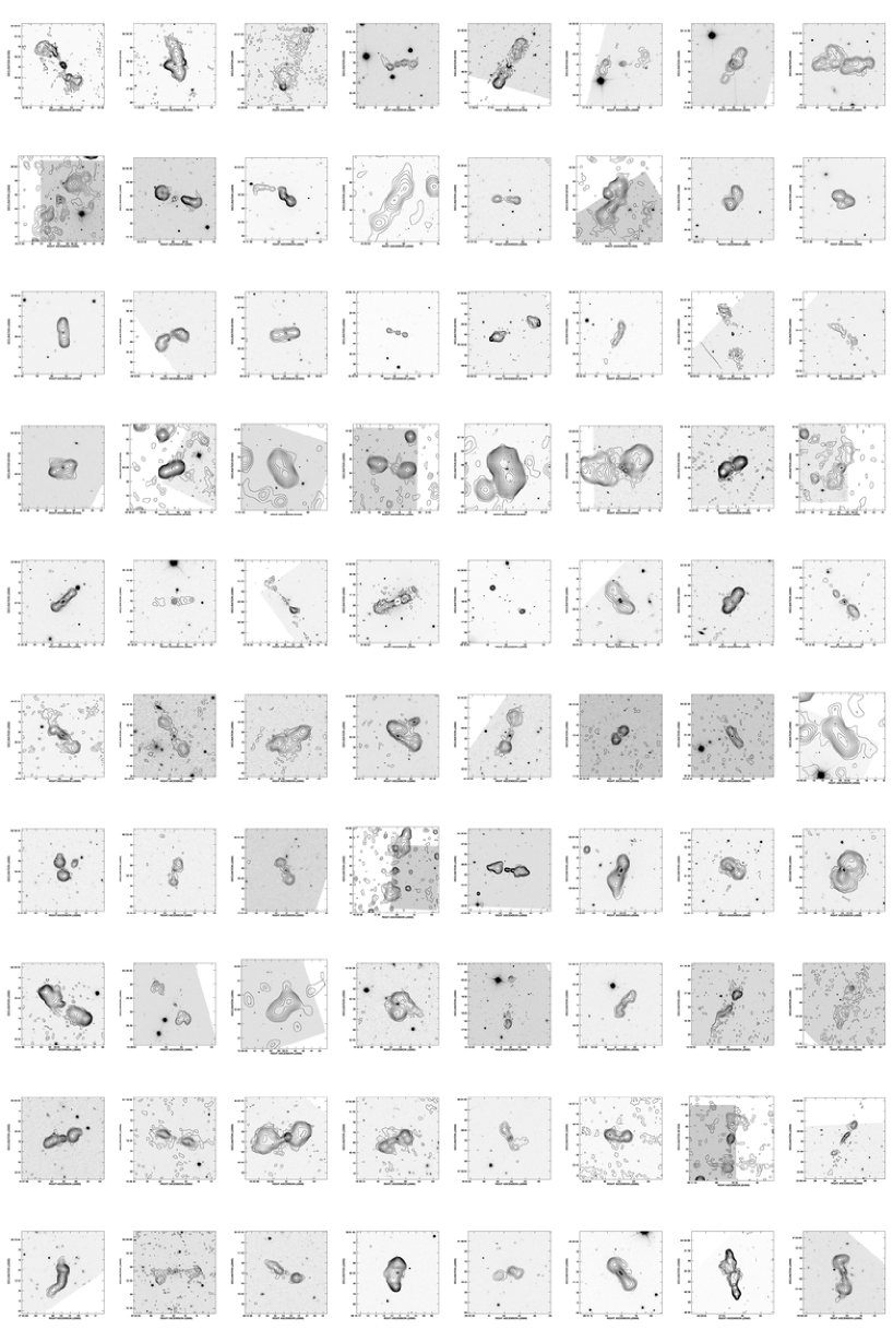
Figure 25: FIRST contour radio maps overplotted on gray scale SDSS r-band images of the first 80 objects from the sample.

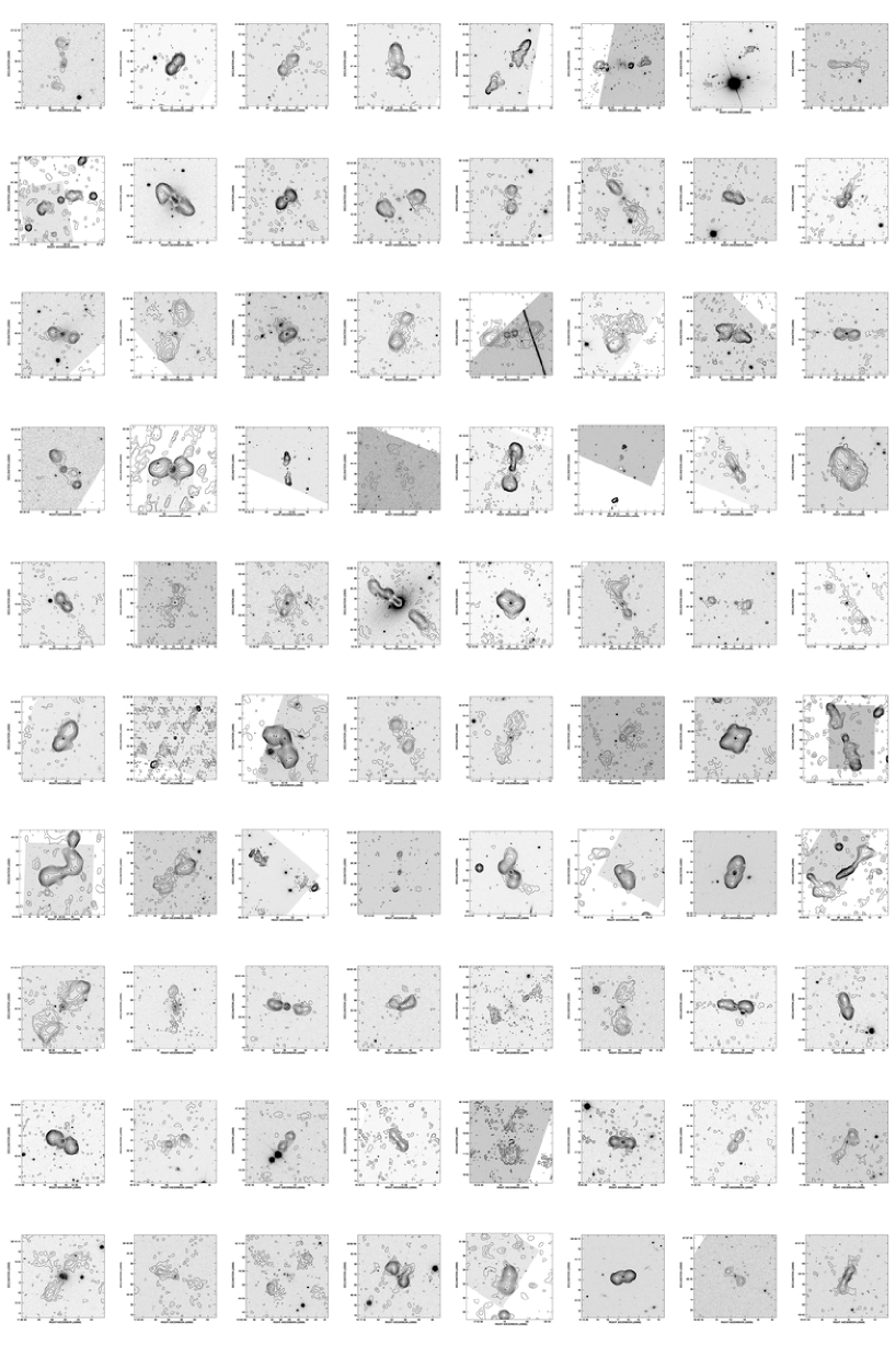
Figure 26: FIRST contour radio maps overploted on gray scale SDSS r-band images of next 80 objects from the sample.

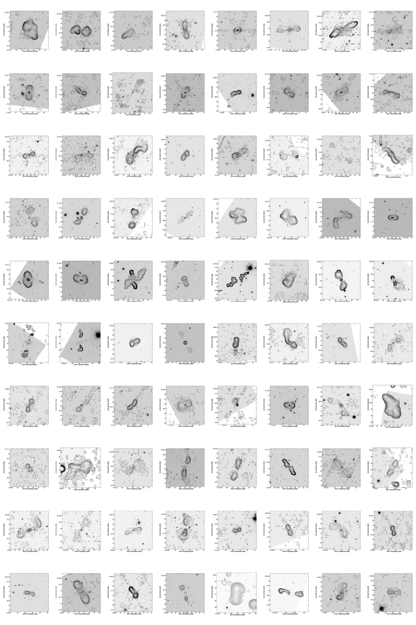
Figure 27: FIRST contour radio maps overploted on gray scale SDSS r-band images of the next 80 objects from the sample.

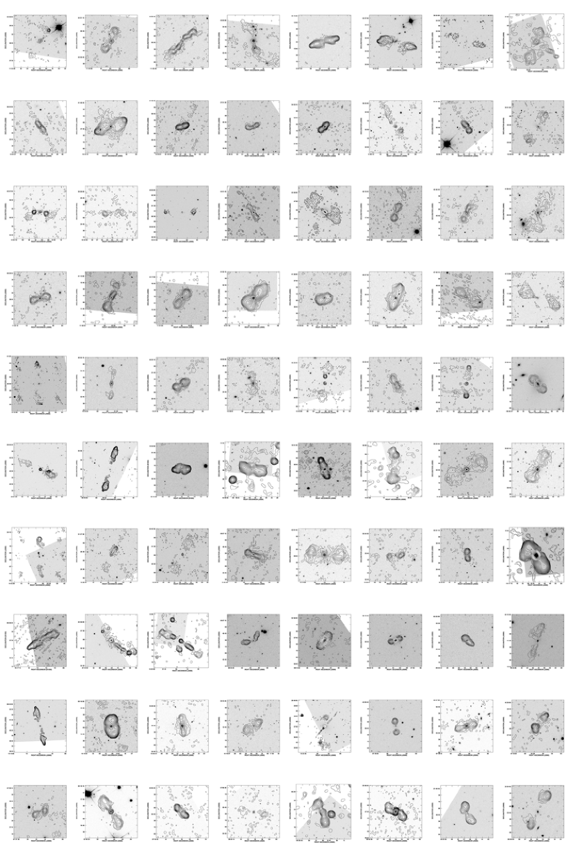
Figure 28: FIRST contour radio maps overploted on gray scale SDSS r-band images of the next 80 objects from the sample.

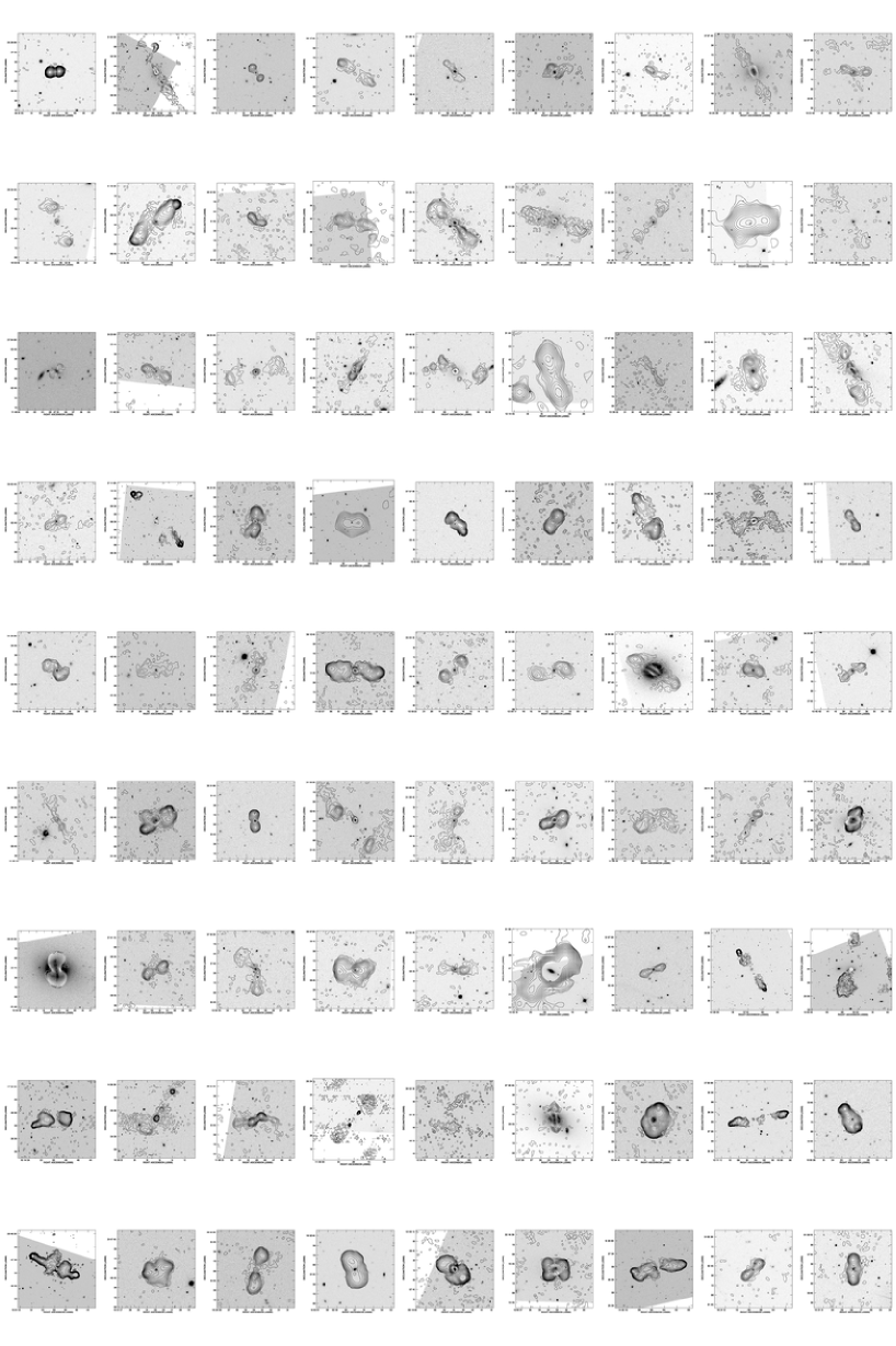
Figure 29: FIRST contour radio maps overploted on gray scale SDSS r-band images of the last 81 objects from the sample.

References

- [\citeauthoryearAbazajian et al.2004] Abazajian K., et al., 2004, AJ, 128, 502
- [\citeauthoryearAbazajian et al.2009] Abazajian K. N., et al., 2009, ApJS, 182, 543
- [\citeauthoryearAkritas & Bershady1996] Akritas M. G., Bershady M. A., 1996, ApJ, 470, 706
- [\citeauthoryearBaldwin et al.1985] Baldwin J. E., Boysen R. C., Hales S. E. G., Jennings J. E., Waggett P. C., Warner P. J., Wilson D. M. A., 1985, MNRAS, 217, 717
- [\citeauthoryearBaldwin, Phillips, & Terlevich1981] Baldwin J. A., Phillips M. M., Terlevich R., 1981, PASP, 93, 5
- [\citeauthoryearBalogh et al.1999] Balogh M. L., Morris S. L., Yee H. K. C., Carlberg R. G., Ellingson E., 1999, ApJ, 527, 54
- [\citeauthoryearBecker, White, & Helfand1995] Becker R. H., White R. L., Helfand D. J., 1995, ApJ, 450, 559
- [\citeauthoryearBell et al.2004] Bell E. F., et al., 2004, ApJ, 608, 752
- [\citeauthoryearBenn1995] Benn C. R., 1995, MNRAS, 272, 699
- [\citeauthoryearBenn & Kenderdine1991] Benn C. R., Kenderdine S., 1991, MNRAS, 251, 253
- [\citeauthoryearBenn et al.1982] Benn C. R., Grueff G., Vigotti M., Wall J. V., 1982, MNRAS, 200, 747
- [\citeauthoryearBennett1962] Bennett A. S., 1962, MmRAS, 68, 163
- [\citeauthoryearBertelli et al.1994] Bertelli G., Bressan A., Chiosi C., Fagotto F., Nasi E., 1994, A&AS, 106, 275
- [\citeauthoryearBest et al.2005a] Best P. N., Kauffmann G., Heckman T. M., Ivezić Ž., 2005, MNRAS, 362, 9
- [\citeauthoryearBest et al.2005b] Best P. N., Kauffmann G., Heckman T. M., Brinchmann J., Charlot S., Ivezić Ž., White S. D. M., 2005, MNRAS, 362, 25
- [\citeauthoryearBruzual A.1983] Bruzual A. G., 1983, ApJ, 273, 105
- [\citeauthoryearBruzual & Charlot2003] Bruzual G., Charlot S., 2003, MNRAS, 344, 1000
- [\citeauthoryearButtiglione et al.2010] Buttiglione S., Capetti A., Celotti A., Axon D. J., Chiaberge M., Macchetto F. D., Sparks W. B., 2010, A&A, 509, A260000
- [\citeauthoryearButtiglione et al.2009] Buttiglione S., Capetti A., Celotti A., Axon D. J., Chiaberge M., Macchetto F. D., Sparks W. B., 2009, A&A, 495, 1033
- [\citeauthoryearChabrier2003] Chabrier G., 2003, PASP, 115, 763
- [\citeauthoryearCid Fernandes et al.2005] Cid Fernandes R., Mateus A., Sodré L., Stasińska G., Gomes J. M., 2005, MNRAS, 358, 363
- [\citeauthoryearCid Fernandes et al.2009] Cid Fernandes R., et al., 2009, RMxAC, 35, 127
- [\citeauthoryearCid Fernandes et al.2010] Cid Fernandes R., Stasińska G., Schlickmann M. S., Mateus A., Vale Asari N., Schoenell W., Sodré L., 2010, MNRAS, 403, 1036
- [\citeauthoryearCondon et al.1998] Condon J. J., Cotton W. D., Greisen E. W., Yin Q. F., Perley R. A., Taylor G. B., Broderick J. J., 1998, AJ, 115, 1693
- [\citeauthoryearEdge et al.1959] Edge D. O., Shakeshaft J. R., McAdam W. B., Baldwin J. E., Archer S., 1959, MmRAS, 68, 37
- [\citeauthoryearFanaroff & Riley1974] Fanaroff B. L., Riley J. M., 1974, MNRAS, 167, 31P
- [\citeauthoryearFitzpatrick1999] Fitzpatrick E. L., 1999, PASP, 111, 63
- [\citeauthoryearGower, Scott, & Wills1967] Gower J. F. R., Scott P. F., Wills D., 1967, MmRAS, 71, 49
- [\citeauthoryearHales, Baldwin, & Warner1993] Hales S. E. G., Baldwin J. E., Warner P. J., 1993, MNRAS, 263, 25
- [\citeauthoryearHales, Baldwin, & Warner1988] Hales S. E. G., Baldwin J. E., Warner P. J., 1988, MNRAS, 234, 919
- [\citeauthoryearHales et al.1990] Hales S. E. G., Masson C. R., Warner P. J., Baldwin J. E., 1990, MNRAS, 246, 256
- [\citeauthoryearHales et al.1993] Hales S. E. G., Masson C. R., Warner P. J., Baldwin J. E., Green D. A., 1993, MNRAS, 262, 1057
- [\citeauthoryearHales et al.1991] Hales S. E. G., Mayer C. J., Warner P. J., Baldwin J. E., 1991, MNRAS, 251, 46
- [\citeauthoryearHales et al.2007] Hales S. E. G., Riley J. M., Waldram E. M., Warner P. J., Baldwin J. E., 2007, MNRAS, 382, 1639
- [\citeauthoryearHales et al.1995] Hales S. E. G., Waldram E. M., Rees N., Warner P. J., 1995, MNRAS, 274, 447
- [\citeauthoryearHardcastle et al.1998] Hardcastle M. J., Alexander P., Pooley G. G., Riley J. M., 1998, MNRAS, 296, 445
- [\citeauthoryearHine & Longair1979] Hine R. G., Longair M. S., 1979, MNRAS, 188, 111
- [\citeauthoryearJanda2006] Janda, K. 2006, MSc Dissertation, Jagiellonian University, Krakow
- [\citeauthoryearKaiser, Schoenmakers, Röttgering2000] Kaiser C. R., Schoenmakers A. P., Röttgering H. J. A., 2000, MNRAS, 315, 381
- [\citeauthoryearKauffmann, Heckman, & Best2008] Kauffmann G., Heckman T. M., Best P. N., 2008, MNRAS, 384, 953
- [\citeauthoryearKauffmann & Heckman2009] Kauffmann G., Heckman T. M., 2009, MNRAS, 397, 135
- [\citeauthoryearLe Borgne et al.2003] Le Borgne J.-F., et al., 2003, A&A, 402, 433
- [\citeauthoryearLedlow & Owen1996] Ledlow M. J., Owen F. N., 1996, AJ, 112, 9
- [\citeauthoryearLin et al.2010] Lin Y.-T., Shen Y., Strauss M. A., Richards G. T., Lunnan R., 2010, ApJ, 723, 1119
- [\citeauthoryearLiu et al.2010] Liu X., Greene J. E., Shen Y., Strauss M. A., 2010a, ApJ, 715, L30
- [\citeauthoryearLiu et al.2010] Liu X., Shen Y., Strauss M. A., Greene J. E., 2010b, ApJ, 708, 427
- [\citeauthoryearMachalski, Koziel-Wierzbowska, & Jamrozy2007] Machalski J., Koziel-Wierzbowska D., Jamrozy M., 2007, AcA, 57, 227
- [\citeauthoryearMarecki & Swoboda2011] Marecki A., Swoboda B., 2011, A&A, 525, A6
- [\citeauthoryearMateus et al.2006] Mateus A., Sodré L., Cid Fernandes R., Stasińska G., Schoenell W., Gomes J. M., 2006, MNRAS, 370, 721
- [\citeauthoryearOwen & Laing1989] Owen F. N., Laing R. A., 1989, MNRAS, 238, 357
- [\citeauthoryearOwen & Ledlow1994] Owen F. N., Ledlow M. J., 1994, ASPC, 54, 319
- [\citeauthoryearPearson1975] Pearson T. J., 1975, MNRAS, 171, 475
- [\citeauthoryearPearson & Kus1978] Pearson T. J., Kus A. J., 1978, MNRAS, 182, 273
- [\citeauthoryearPierce et al.2010] Pierce C. M., et al., 2010, MNRAS, 405, 718
- [\citeauthoryearPilkington & Scott1965] Pilkington J. D. H., Scott P. F., 1965, MmRAS, 69, 183
- [\citeauthoryearRawlings et al.1989] Rawlings S., Saunders R., Eales S. A., Mackay C. D., 1989, MNRAS, 240, 701
- [\citeauthoryearRees1990] Rees N., 1990, MNRAS, 244, 233
- [\citeauthoryearSchinnerer et al.2007] Schinnerer E., et al., 2007, ApJS, 172, 46
- [\citeauthoryearSmolčić et al.2009] Smolčić V., et al., 2009, ApJ, 696, 24
- [\citeauthoryearSmolčić2009] Smolčić V., 2009, ApJ, 699, L43
- [\citeauthoryearSpergel et al.2003] Spergel D. N., et al., 2003, ApJS, 148, 175
- [\citeauthoryearStasińska et al.2006] Stasińska G., Cid Fernandes R., Mateus A., Sodré L., Asari N. V., 2006, MNRAS, 371, 972 (S06)
- [\citeauthoryearTremaine et al.2002] Tremaine S., et al., 2002, ApJ, 574, 740
- [\citeauthoryearWaldram et al.2003] Waldram E. M., Pooley G. G., Grainge K. J. B., Jones M. E., Saunders R. D. E., Scott P. F., Taylor A. C., 2003, MNRAS, 342, 915
- [\citeauthoryearYork et al.2000] York D. G., et al., 2000, AJ, 120, 1579
- [\citeauthoryearZirbel & Baum1995] Zirbel E. L., Baum S. A., 1995, ApJ, 448, 521