Traffic properties for stochastic routings on scale-free networks

Abstract

For realistic scale-free networks, we investigate the traffic properties of stochastic routing inspired by a zero-range process known in statistical physics. By parameters $\alpha$ and $\delta$, this model controls degree-dependent hopping of packets and forwarding of packets with higher performance at more busy nodes. Through a theoretical analysis and numerical simulations, we derive the condition for the concentration of packets at a few hubs. In particular, we show that the optimal $\alpha$ and $\delta$ are involved in the trade-off between a detour path for $\alpha<0$ and long wait at hubs for $\alpha>0$; In the low-performance regime at a small $\delta$, the wandering path for $\alpha<0$ better reduces the mean travel time of a packet with high reachability. Although, in the high-performance regime at a large $\delta$, the difference between $\alpha>0$ and $\alpha<0$ is small, neither the wandering long path with short wait trapped at nodes ($\alpha=-1$), nor the short hopping path with long wait trapped at hubs ($\alpha=1$) is advisable. A uniformly random walk ($\alpha=0$) yields slightly better performance. We also discuss the congestion phenomena in a more complicated situation with packet generation at each time step.

I Introduction

In daily socio-economic network systems, many commodities, passengers, or information fragments (abstractly referred to as packets in this paper) are delivered from one place to another place. In general, it is expected to send and receive packets as quickly as possible without encountering traffic congestion which would force packets to wait at nodes. Even if packets are concentrated (or condensed in term of statistical physics) on just a few nodes in some parts of a network, this situation may cause congestion over the network. Thus, one of the important issues is a routing strategy: how to select a forwarding node in the neighbors of the resident node of a packet. Since the efficiency of transportation or communication depends on not only routing strategy, but also on network topology, we should consider a realistic problem setting for the routing and the topology. In addition, considering the interaction of accumulated packets in a buffer (called queue) at each node is necessary, since it crucially affects the traffic flow on a network. This paper discusses traffic properties that depend on routing strategies in the interaction of packets on a realistic network topology.

During this decade, a new research field, complex network science, has been created Albert02 , since a common topological structure called scale-free (SF) was found to exist in many real networks such as the Internet, the World-Wide-Web, power grids, airline networks, social collaboration networks, human sexual contacts, and biological metabolic pathways, etc. The SF structure is characterized by the property that the distribution of degree (the number of connections to a node) follows a power-law. In other words, the network consists of many nodes with low degrees and a few hubs with high degrees. Moreover, a SF network naturally emerges in social acquaintance relationships or peer-to-peer communications, and it has short paths compared with large network size (the total number of nodes).

In a realistic SF network, a routing path is shortened by passing through hubs for the forwarding of a packet. However, many packets may be concentrated at the hubs Goh01 , in whose queues the packets are cumulatively stored if they arrive in a quantity larger than the processing limit for forwarding. In such a situation, there exists a trade-off between delivering packets on a short path and avoiding traffic congestion. To improve communication efficiency even in a dynamic environment for a wireless or ad hoc network, various routing schemes are being developed. Because, in an ad hoc network, many nodes (such as base stations or communication sites) and connections between them are likely to change over time, then global information, e.g., a routing table in the Internet, cannot be applied. In early work, some decentralized routing developed to reduce energy consumption in sensor or mobile networks, however they lead to the failure of guaranteed delivery Urrutia02 ; in the flooding algorithm, multiple redundant copies of a message are sent and cause congestion, while greedy and compass routing may occasionally fall into infinite loops or into a dead end. Thus, we focus on stochastic routing methods using only local information with respect to the resident node of a packet and to the connected neighbors on a path, due to their simplicity and power. If the terminal node of a packet is included in the neighbors of the resident node, then the packet is deterministically sent to the terminal in order to guarantee reachability unless the connectivity is broken. We call this neighbor search (or n-search) only at the last step to the terminal. Note that the development of stochastic routing methods is still in progress depending on device and information processing technologies. Although we suppose a mixture of wireless and wired communications in future networks, first of all, we aim to understand the relations for traffic properties between fixed network topology and routing methods. Here, it is usually assumed for simplicity that each node has the same performance in the forwarding of packets.

The enhancement of performance in forwarding is also reasonable Liu06 ; Zhao05 . For example, in the Internet or airline networks, an important facility with many connections has high performance; more packets or flights are processed as the incoming flux of communication requests or of passengers increases. Such higher performance at more busy nodes is effectively applied in a zero-range process (ZRP) Noh05a ; Noh05b , which tends to distribute packets throughout the whole network, instead of avoiding paths through hubs.

In this paper, from the random walk version, we extend the ZRP on a SF network to the degree-dependent hopping rule, which parametrically controls routing strategies in the trade-off between the selection of a short path passing through hubs, and the avoidance of hubs at which many packets are condensed and wait in queues for a long time. The above models in statistical physics are useful for the analysis of complex phenomena involved in transition form a free-flow phase to a congestion phase, or the opposite transition. Most research on traffic congestion rely on numerical simulations. Although a few other theoretical analyses based on the mean-field approximation Martino09 have been done, we can not compare them to the ZRP, simply because of different problem settings. Thus, we consider a combination of settings as modified traffic models, and numerically investigate them.

The organization of this paper is as follows. In Sec. II, we briefly review the related models in recent studies. In Sec. III, we introduce a stochastic packet transfer model defined by the ZRP, in which all packets persist without any generation and removals. Then, in terms of fundamental properties, we approximately analyze the stationary probability of incoming packets at each node on SF networks, and derive the phase transition for condensation of packets at hubs in the degree-dependent hopping rule. In Sec. IV, we numerically confirm the phase transition, and as a new result, show the trade-off between a detour wandering path and long wait at hubs. Moreover, we discuss the congestion phenomenon in the modified traffic models with packet generation. In Sec. V, we summarize these results and describe some issues for further research.

II Related Work

Many traffic models have been proposed in various problem settings for routing, node capacity, and packet generation. They are summarized in Table 1. The basic processes for packet transfer consist of the selection of a forwarding (coming-in) node and the jumping-out of packets in the node capacity. In these models (including our model discussed later), a significant issue commonly arises from the trade-off between delivering packets on a shorter path and avoiding the congestion caused by a concentration of packets on a few nodes such as hubs.

In the typical models, a forwarding node $k$ is chosen with probability either $K_{k}^{\alpha}/\sum_{j\in{\cal N}_{i}}K_{j}^{\alpha}$ Yamashita03 ; Wang06a ; Yan06 or $(m_{(k)}+1)^{-\beta}/\sum_{j\in{\cal N}_{i}}(m_{(j)}+1)^{-\beta}$ Danila06 . Here, $\alpha$ and $\beta$ are real parameters, $K_{k}$ and $m_{(k)}$ denote the degree and the dynamically-occupied queue length by packets at node $k$ in the connected neighbors ${\cal N}_{i}$ to the resident node $i$ of the packet. These methods are not based on a random walk (selecting a forwarding node uniformly at random among the neighbors), but on the extensions (including the uniformly random one at $\alpha,\beta=0$) called preferential and congestion-aware walks, respectively. Note that $\alpha>0$ leads to a short path passing through hubs, and that $\alpha<0$ and $\beta>0$ lead to the avoidance of hubs and congested nodes with large $m_{(k)}$. In stochastic routing methods, instead of using the shortest path, the optimal values $\alpha=-1$ and $\beta=1$ for maximizing the generation rate of packets in a free-flow regime have been obtained by numerical simulations Wang06a ; Yan06 . A correlation between the congestion at node level and a betweenness centrality measure was suggested Danila06 .

Other routing schemes Wang06b ; Echenique05 ; Martino09 have also been considered, taking into account lengths of both the routing path and of the queue. In a deterministic model Echenique05 , a forwarding node $k$ is chosen among neighbors ${\cal N}_{i}$ by minimizing the quantity $hd_{k}+(1-h)m_{(k)}$ with a weight $0\leq h\leq 1$, $d_{k}$ denoting the distance from $k$ to the terminal node. Since we must solve the optimization problems, these models Yan06 ; Echenique05 are not suitable for wireless or ad hoc communication networks. Thus, stochastic routing methods using only local information are potentially promising. In a stochastic model Martino09 , $k\in{\cal N}_{i}$ is chosen at random, and a packet at the top of its queue is sent with probability $1-\eta(m_{(k)})$ or refused with probability $\eta(m_{(k)})$ as a nondecreasing function of the queue length $m_{(k)}$. This model is simplified by the assumption of a constant arrival rate of packets, for analyzing the critical point of traffic congestion in a mean-field equation Martino09 .

With a different processing power at each node Wang06a , it has also been considered that the node capacity $c_{i}$ is proportional to its degree $K_{i}$, therefore more packets jump out from a node as the degree becomes larger. On the other hand, in the ZRP Noh05a ; Noh05b ; Noh07 , the forwarding capacity at a node depends on the number of $m_{(i)}$ defined as a queue length occupied by packets at node $i$. The ZRP is a solvable theoretical model for traffic dynamics. In particular, in the ZRP with a random walk at $\alpha=0$, the phase transition between condensation of packets at hubs and uncondensation on SF networks has been derived Noh05a ; Noh05b . For $\alpha>0$, a similar phase transition has been analyzed in the mean-field approximation Tang06 .

In the next two sections, based on a straightforward approach introduced in Refs. Noh05a ; Noh05b , we derive the phase transition in the ZRP on SF networks with the degree-dependent hopping rule for both $\alpha>0$ and $\alpha<0$, inspired by preferential Yamashita03 ; Wang06a ; Yan06 and congestion-aware walks. Although the rule is not identical to the congestion-aware routing scheme Danila06 based on occupied queue length $m_{(k)}$, $\alpha<0$ corresponds to avoiding hubs with large degrees, where many packets tend to be concentrated. Furthermore, we study the traffic properties in the case with neighbor search into a terminal node at the last step.

Table 1: Recent traffic models for complex networks. When a packet is forwarded from a current node $i$ to $k\in{\cal N}_{i}$, the neighboring node $k$ is chosen with probability $\Pi_{k}$ or by minimizing an objective function on a routing path. The node capacity $c_{i}$ is defined by the number of simultaneously transferable packets from each node $i$. Here, $K(x_{l})$ denotes the degree of node $x_{l}$, $\Theta(x)$ is the step function, and $m^{*}$ is a threshold, $\beta\geq 0$, and $0\leq\bar{\eta}<1$.

Ref.	selection of	node	packet
	forwarding node	capacity	generation
Wang06a	$\Pi_{k}\propto K_{k}^{\alpha}$	$c_{i}=10$ or	Yes
	$-1\leq\alpha\leq 1$	$c_{i}=K_{i}$
Yan06	$\min\;\sum_{l}K(x_{l})^{\beta}$	$c_{i}=1$	Yes
	on a path $\{x_{0},\ldots,x_{n}\}$
Danila06	$\Pi_{k}\propto(m_{(k)}+1)^{-\beta}$	$c_{i}=1$	Yes
Wang06b	$\Pi_{k}\propto K_{k}(m_{(k)}+1)^{-\beta}$	$c_{i}=5$	Yes
Echenique05	$\min\;hd_{k}+(1-h)m_{(k)}$	$c_{i}=1$	Yes
	$0\leq h\leq 1$
Martino09	random walk
	with a refusal prob.	$c_{i}=1$	Yes
	$\bar{\eta}\Theta(m_{(k)}-m^{*})$
Noh05a ; Noh05b ; Noh07	$\Pi_{k}\propto K_{k}^{\alpha}$	jumping rate	No
Tang06	$\alpha>0$	$m_{(i)}^{\delta}$

III Packet Transfer Model

III.1 Routing rule

Consider a system of $M$ interacting packets on a network of $N$ nodes with a density $\rho=M/N$, $M=\sum_{i=1}^{N}m_{(i)}$, where $m_{(i)}\geq 0$ denotes the occupation number of packets in the queue at each node $1\leq i\leq N$. For simplicity, we assume that the queue length is not limited, and that the order of stored packets is ignored. If there is a limitation on the queue length, it may become necessary to discuss a cascading problem Motter02 ; Motter04 ; Wu07 whose dynamics are very complicated.

To investigate the predicted properties from the theoretical analysis in the ZRP Noh05a ; Noh05b ; Noh07 , we use the same problem setting, such that all packets persist on paths in the network without generation or removals of packets. For more complex situations with packet generation, some models modified by adding different routing rules will be investigated in subsection 4.2.

In this routing rule related to the ZRP, the total number $M$ of packets is constant at any time, and each node performs a stochastic local search as follows: at each time step, a packet jumps out of a node $i$ stochastically at a given rate $q_{i}(m_{(i)})$ as a function of $m_{(i)}$, and then comes into one of the neighboring nodes $k\in{\cal N}_{i}$ chosen with probability $K_{k}^{\alpha}/\sum_{k^{\prime}\in{\cal N}_{i}}K_{k^{\prime}}^{\alpha}$. When a packet is transferred from $i$ to $k$, the queue length $m_{(k)}$ is increased by one unit, and $m_{(i)}$ is simultaneously decreased. The above processes are conceptual, the relaxation dynamics for the simulation of packet transfer is necessary, and described in Sec. IV. The effect of the deterministic neighbor search into a terminal node at the last step will also be discussed later.

III.2 Stationary probability in $\alpha$-random walks

Before investigating the influence of dynamic queue lengths on traffic properties, we consider the stationary probability of incoming packets at each node. As mentioned in the previous subsection, we extend a random walk routing Noh07 ; Noh04 , in which a walker (packet) chooses a node uniformly at random among the neighbors of the current node on a path, to a degree-dependent routing. We call it $\alpha$-random walk.

As in Ref. Noh04 , for the probability $P_{ij}$ of finding the walker at node $j\in{\cal N}_{k}$ from node $i$ through the intermediate nodes $k\in{\cal N}_{i}$ at time $t$, the master equation is

$$P_{ij}(t+1)=\sum_{k}\frac{K_{j}^{\alpha}}{\sum_{j^{\prime}\in{\cal N}_{k}}K_{j^{\prime}}^{\alpha}}P_{ik}(t).$$ (1)

By iterating Eq. (1), an explicit expression for the transition probability $P_{ij}$ to go from node $i$ through $j_{1},\ldots,j_{t-1}$ to $j$ in $t$ steps follows as

$$P_{ij}(t)=\sum_{j_{1},\ldots,j_{t-1}}\frac{K_{j_{1}}^{\alpha}}{\sum_{j^{\prime}_{1}\in{\cal N}_{i}}K_{j^{\prime}_{1}}^{\alpha}}\times\ldots\times\frac{K_{j}^{\alpha}}{\sum_{j^{\prime}\in{\cal N}_{j_{t-1}}}K_{j^{\prime}}^{\alpha}},$$ (2)

where the sum $\sum_{j_{1},\ldots,j_{t-1}}$ is taken over the connected paths between nodes $i$ and $j$, as shown in Fig. 1. In the opposite directions of the same paths, the transition probability $P_{ji}$ follows as

$$P_{ji}(t)=\sum_{j_{t-1},\ldots,j_{1}}\frac{K_{j_{t-1}}^{\alpha}}{\sum_{j^{\prime}_{t-1}\in{\cal N}_{j}}K_{j^{\prime}_{t-1}}^{\alpha}}\times\ldots\times\frac{K_{i}^{\alpha}}{\sum_{i^{\prime}\in{\cal N}_{j_{1}}}K_{i^{\prime}}^{\alpha}}.$$ (3)

We assume the network to be uncorrelated: there is no correlation between two degrees of any connected nodes, so that $\sum_{j^{\prime}_{1}}K_{j^{\prime}_{1}}^{\alpha}=K_{i}\cdot\langle K^{\alpha}\rangle$ and $\sum_{j^{\prime}_{t-1}}K_{j^{\prime}_{t-1}}^{\alpha}=K_{j}\cdot\langle K^{\alpha}\rangle$ hold by using the mean value $\langle K^{\alpha}\rangle$ of the $\alpha$-power of degree. By comparing the expression of $P_{ij}$ in Eq. (2) with that of $P_{ji}$ in Eq. (3), we obtain the equivalent relation

$$\frac{K_{i}}{K_{j}^{\alpha}}P_{ij}=\frac{K_{j}}{K_{i}^{\alpha}}P_{ji}.$$

Thus, for any source $i$ and step $t$, $P_{ij}$ is proportional to $K_{j}^{1+\alpha}$, while $P_{ji}$ is proportional to $K_{i}^{1+\alpha}$. Consequently, the stationary solution $P_{j}^{\infty}$ of the incoming probability $P_{ij}$ is proportional to $K_{j}^{1+\alpha}$. This form, related only to the degree of the forwarding node $j$, is suitable for the theoretical analysis of the ZRP presented in the next subsection and in the Appendix. The approximative solution is also obtained from a different approach to the master equation Wang06a under the same assumption of uncorrelated networks.

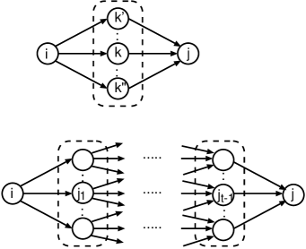
Figure 1: Combination of consecutive nodes on the route from node $i$ to $j$. The dashed rectangles correspond to the sum of Eqs. (1)-(3).

Figure 2 shows the stationary solution $P_{j}^{\infty}\propto K_{j}^{\beta}$ and the exponent $\beta\approx 1+\alpha\geq 0$ for the SF networks (generated by the BA: Barabási-Albert model Albert02 ). Table 2 also shows that the estimated exponents $\beta$ are consistent in the cases both with and without neighbor search into a terminal node at the last step. Here, the terminal is chosen from all nodes uniformly at random. After arriving at the terminal, the packet is restarted (resent) from the node to a new terminal, in order to maintain the persistency of packets in the ZRP.

Figure 2: Probability of incoming at a node with degree $K$ in the $\alpha$-random walk of $M=1000$ independent packets (equivalent to the case of $\delta=1$) through 1000 rounds. The lines guide the estimated slopes in the left column (without n-search) in Table 2, and the plotted marks show the probability obtained in a BA network with $N=1000$ and $\langle K\rangle=10$.

Table 2: Numerically estimated exponent $\beta\approx 1+\alpha$ for the lines from the plotted marks in Fig. 2 by using the mean-square-error method for the independent walks of $M=1000$ packets. These values give the averaged slopes for $P_{j}^{\infty}\propto K_{j}^{\beta}$ in 100 BA networks with $N=1000$ and $\langle K\rangle=10$.

	without	with n-search
$\alpha$	$\beta$	$\beta$
1.0	2.245	2.143
0.5	1.611	1.576
0.0	1.039	1.027
-0.5	0.524	0.519
-1.0	0.022	0.019

III.3 Phase transition in the ZRP

We discuss the phase transition between condensation and uncondensation in the ZRP with degree-dependent hopping rule of packets. For the configuration

$$m_{(1)},\ldots,m_{(i)},\ldots,m_{(N)}$$

of occupation at each node, the stationary solution of a single packet is given by the factorized form

$$P(m_{(1)},\ldots,m_{(i)},\ldots,m_{(N)})=\frac{1}{Z}\Pi_{i=1}^{N}f_{i}(m_{(i)}),$$ (4)

where $Z$ is a normalization factor and

$$f_{i}(m_{(i)})\stackrel{{\scriptstyle\rm def}}{{=}}\Pi_{\omega=1}^{m_{(i)}}\left(\frac{P_{i}^{\infty}}{q_{i}(\omega)}\right),$$ (5)

for an integer $m_{(i)}>0$ and $f_{i}(0)=1$. We consider a function $q_{i}(\omega)=\omega^{\delta}$ with a parameter $0\leq\delta\leq 1$ for forwarding performance. This means that a node works harder for transfer, as it has more packets in the queue with larger $\omega$ and $\delta$.

Using the probability distribution in Eq. (4) and the stationary probability $P_{i}^{\infty}\propto K_{i}^{\beta}$, we can calculate the mean value $\langle m_{(i)}\rangle$ at each node. Here, $\langle m_{(i)}\rangle\stackrel{{\scriptstyle\rm def}}{{=}}\sum_{\omega=0}^{\infty}\omega P_{i}(m_{(i)}=\omega)$ is defined by using the probability distribution $P_{i}(m_{(i))}=\omega)$ of the number of packets occupying node $i$.

$$P_{i}(m_{(i)}=\omega)=\frac{1}{Z_{i}}\sum_{*}f_{i}(\omega)\Pi_{j\neq i}f_{j}(m_{(j)}),$$ (6)

where the sum $\sum_{*}$ is taken in combination $\{m_{(1)},\ldots,m_{(i-1)},m_{(i+1)},\ldots,m_{(N)}\}$ on the constraint $\sum_{j\neq i}m_{(j)}=M-\omega$ as shown in Fig. 3, and $Z_{i}$ is a normalization factor. It is difficult to directly solve the normalization factor $Z_{i}$ or $Z$. Thus, introducing a fugacity variable $z$ Evans00 , the mean value is given by a generating function

$$\langle m_{(i)}\rangle=\frac{\sum_{\omega}\omega z^{\omega}f_{i}(\omega)}{\sum_{\omega}z^{\omega}f_{i}(\omega)}=z\frac{\partial\ln F_{i}(z)}{\partial z},$$ (7)

where the second term in the right-hand side of Eq. (7) is due to the definition

$$F_{i}(z)\stackrel{{\scriptstyle\rm def}}{{=}}\sum_{\omega=0}^{\infty}z^{\omega}f_{i}(\omega).$$

From the definition (5), $q_{i}(\omega)=\omega^{\delta}$, and $P_{i}^{\infty}\propto K_{i}^{\beta}$, we have

$$F_{i}(z)=\sum_{\omega=0}^{\infty}\frac{(zK_{i}^{\beta})^{\omega}}{(\omega\;!)^{\delta}},$$ (8)

because $f_{i}(\omega)=\Pi_{m=1}^{\omega}\left(\frac{K_{i}^{\beta}}{m^{\delta}}\right)=\frac{(K_{i}^{\beta})^{\omega}}{(\omega!)^{\delta}}$ in Eq. (5). The fugacity $z$ should be determined from the self-consistency equation $\rho=\sum_{i=1}^{N}\langle m_{(i)}\rangle/N$ as a function of $z$. Note that $M=\sum_{i=1}^{N}\langle m_{(i)}\rangle$ is the total number of packets in a network of $N$ nodes, and that the density $\rho$ is constant at $N,M\rightarrow\infty$.

In this paper, we consider a SF network whose degree distribution follows a power-law $P(K)\sim K^{-\gamma}$. According to the performances of jumping-out, we classify the following cases (A) $\delta>\delta_{c}\stackrel{{\scriptstyle\rm def}}{{=}}\beta/(\gamma-1)$, (B) $\delta=\delta_{c}$, (C) $\delta<\delta_{c}$, and (D) $\delta=0$ for a critical value $\delta_{c}$ of the phase transition from uncondensation to condensation of packets, or the opposite transition. Since the derivation is the same as in Refs. Noh05a ; Noh05b at $\alpha=0$, except with a slight modification for a general value of $\alpha$ (and the corresponding $\beta\approx 1+\alpha$), we briefly review it in the Appendix. We summarize the generalized results for $0\leq|\alpha|\leq 1$ in Table 3 (from that for $\alpha=0$). In the cases (B) and (C), many packets condensate at nodes with degree $K>K_{c}$ because of the larger exponent $\beta/\delta>\beta$. Note that the queue length occupied by packets is rewritten as $m_{K_{i}}$ taking into account the dependence on the degree $K_{i}$.

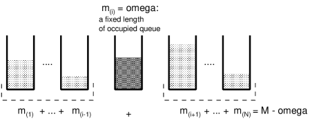
Figure 3: Illustration of the queue length occupied by packets at each node. For the sum $\sum_{*}$ in Eq. (6), there are many combinations of $\{m_{(1)},\ldots,m_{(i-1)},m_{(i+1)},\ldots,m_{(N)}\}$ satisfying $\sum_{j\neq i}m_{(j)}=M-\omega$.

Table 3: Scaling of the crossover degree $K_{c}$, the mean occupation number $m_{K}$ at a node with degree $K$ and $m_{hub}$ at the hub with the maximum degree $K_{max}$ for the cases: (A) $\delta>\delta_{c}$, (B) $\delta=\delta_{c}$, (C) $0<\delta<\delta_{c}$, and (D) $\delta=0$. A blank denotes no correspondence.

	$K_{c}$	$m_{K<K_{c}}$	$m_{K>K_{c}}$	$m_{hub}$
(A)			$K^{\beta/\delta}$	$O(N^{\delta_{c}/\delta})$
(B)	$(\ln K_{max})^{\delta_{c}/\beta}$	$(K/K_{c})^{\beta}$	$(K/K_{c})^{\beta/\delta_{c}}$	$O(N/\ln N)$
(C)	$K_{max}^{1-\delta/\delta_{c}}$	$(K/K_{c})^{\beta}$	$(K/K_{c})^{\beta/\delta}$	$O(N)$
(D)	$K_{max}$	$K^{\beta}/(K_{max}^{\beta}-K^{\beta})$		$\rho N$

IV Simulation

In subsection 4.1, we numerically investigate the basic properties of packet transfer in the ZRP. In subsection 4.2, we further discuss congestion phenomena with packet generation.

IV.1 Traffic properties for $\alpha$-random walks in the ZRP

We have performed simulations for $M=1000$ packets on SF networks generated by the BA model Albert02 with a size $N=1000$, an average degree $\langle K\rangle=10$, and an exponent $\gamma=3$ of $P(K)\sim K^{-\gamma}$. From the initial state in which one packet is set on each node, the following processes are repeated as the relaxation of the ZRP Noh05b from node-based dynamics to particle-based dynamics Evans00 . At each time step, a packet is selected at random. With probability $q_{i}(m_{(i)})/m_{(i)}=m_{(i)}^{\delta-1}$, the packet jumps out of its resident node $i$, and hops to one of the neighboring nodes $j\in{\cal N}_{i}$ with probability $K_{j}^{\alpha}/\sum_{j^{\prime}\in{\cal N}_{i}}K_{j^{\prime}}^{\alpha}$. Otherwise, the selected packet does not move with probability $1-q_{i}(m_{(i)})/m_{(i)}$. The time is measured as a unit of one round (Monte Carlo sweep) consisting of $M$ trials of the random selection of a packet.

Table 4: Classification of the cases in Table 3 for the combinations of $\alpha$ and $\delta$. The values in the mid-columns are $K_{c}=K_{max}^{1-\delta/\delta_{c}}$, for $\delta_{c}=\beta/2$ in the case (C), corresponding to the maximum, average, and minimum of $K_{max}=189,132,98$ in each vertical triplet from the top to the bottom. These results are obtained in 100 realizations of BA networks with $N=1000$ and $\langle K\rangle=10$.

	$\delta$		0.0	0.2	0.5	0.8	$\delta_{c}$
$\alpha$
				74.26	18.29	4.504
1.0			(D)	55.29	14.98	4.063	1.122
				43.28	12.71	3.731
				51.44	7.304	1.037
0.5			(D)	39.27	6.374	1.034	0.805
				31.39	5.693	1.032
				25.15	1.221
0.0			(D)	20.16	1.204	(A)	0.519
				16.79	1.191
				3.478
-0.5			(D)	3.193	(A)	(A)	0.262
				2.975
-1.0			(D)	(A)	(A)	(A)	0.011

Case(C): $\alpha=0.5$, $\delta=0.2$

Case(A): $\alpha=-0.5$, $\delta=0.8$

Figure 4: Typical results for the mean occupation number $\langle m_{K}\rangle$ of packets at a node with degree $K$ in the routing without n-search. Inset: the cases with n-search. The circle and cross marks correspond to the results in 1000 and 100 rounds, respectively. The dashed lines show the slopes $\beta$ and $\beta/\delta$ in Table 3. Note that condensation of packets at the nodes with high degrees occurs in Case(C). These results are obtained from the averages of 100 samples of packet transfer on a BA network whose maximum degree is the closest to the average value $K_{max}=132$ in the 100 realizations.

Figure 4 shows the mean occupation number $\langle m_{K}\rangle$ of packets at a node with degree $K$ in the cases both with/without neighbor search (n-search), while the top of Fig. 4 shows the predicted piecewise linear behavior Tang06 for the crossover degree $K_{c}$ shown in Table 4; the steeper line indicates condensation at the nodes with high degrees, and the bottom of Fig. 4 shows that condensation is suppressed by a more gentle line. As shown in the insets, the marks slightly deviate from a line, especially in the head and the tail, because of the effect of n-search into a terminal node at the last step. In these cases at the top and the bottom of Fig. 4, the critical values of $\delta_{c}\approx(1+\alpha)/(\gamma-1)$ are $0.75>\delta$ and $0.25<\delta$, respectively. Thus, condensation of packets at hubs can be avoided as the performance of transfer is enhanced at a large $\delta$, although the transition depends on the probability of incoming packets according to the value of $\alpha$; a negative $\alpha$ induces a nearly homogeneous visiting of nodes, while a positive $\alpha$ induces a heterogeneously biased visiting of the nodes with high degrees. We note that the uncondensed phase is maintained in a wide range of $\delta>\delta_{c}\approx(1+\alpha)/(\gamma-1)$ for $\alpha<0$, as shown in the case (A) of Table 4.

Next, in order to study the traffic properties, such as the travel time on the routing path, we consider packet dynamics in a realistic situation with n-search into a terminal node at the last step. If the terminal is included among the neighbors of the resident node for a randomly selected packet, then it is deterministically forwarded to the terminal node, taking into account the reachable chance, otherwise it is stochastically forwarded to a neighboring node $j$ with probability $K_{j}^{\alpha}/\sum_{j^{\prime}\in{\cal N}_{i}}K_{j^{\prime}}^{\alpha}$. The n-search is practically effective and necessary in order to reach a terminal node. Remember that the estimated values of $\beta$ are similar to both with/without n-search, as shown in Table 2. Therefore, the behavior of the mean occupation number $\langle m_{K}\rangle$ is similar to that shown in Fig. 4 and the inset. In the following discussions, if we leave out n-search, then the optimal parameter values of $\alpha$ and $\delta$ may be changed for low-latency delivery, although the difference is probably small from the above similarity. By selecting hubs for $\alpha>0$, a packet is terminated with higher probability even in only the stochastic forwarding, because a terminal node is highly likely to be connected to some hubs. At the same time, this leads to congestion at hubs. However, in the case without n-search, a packet may wander for a very long time, which is not bounded a priori for the simulation of the packet transfer. It is intractable due to huge computations. Thus, we focus on the case with n-search.

We investigate the traffic properties for reachability of packets, the number of hops, the travel time $T_{a}$ including the wait time of a trapped packet in queues, and the sum $T_{w}$ of wait times on a path until arrival at the terminal. Note that the travel time is $T_{a}=T_{w}\;\;+$ (time to one hop)$\times$(the number of hops). We also define the averaged wait time $T_{w}/N_{w}$ per node, where $N_{w}$ is the number of trappings in queues at the nodes on a routing path. These measures are cumulatively counted in the observed interval after 1000 rounds, and averaged over 100 samples of this simulation. Here, we discarded the initial 1000 rounds as a transient before the stationary state of $m_{(i)}$ is reached.

Figure 5: Convergence properties in the high-performance regime at $\delta=0.8$ in the observed interval [rounds] after the transient state of $\langle m_{K}\rangle$. Inset: results in the low-performance regime at $\delta=0.0$. These results are obtained from the averages of 100 samples of packet transfers on a BA network whose maximum degree is the closest to the average value $K_{max}=132$ in the 100 realizations.

Figure 6: The mean travel time (top) and the mean number of hops (bottom). The $\bigtriangleup$, $+$, $\ast$, $\times$, and $\bigtriangledown$ marks correspond to $\alpha=1.0,0.5,0.0,-0.5$, and $-1.0$, respectively. The simulation conditions are the same as in Fig. 5.

Figure 5 shows, from the top to the bottom, the convergence of reachability, the mean number of restarted packets per round, and the mean travel time in the high-performance regime at $\delta=0.8$. The inset shows a slightly slow convergence in the low-performance regime at $\delta=0.0$. For other measures, similar convergence properties are obtained. We compare these curves in terms of the values of $\alpha$; they shift up from $\alpha=-1.0$ to $\alpha=0.5$ in the case (A) $\delta>\delta_{c}$, while down from $\alpha=0.5$ to $\alpha=1.0$ in the case (C) $\delta<\delta_{c}$. This non-monotonic dependence on $\alpha$ is related to the condensation transition, since the change between $\delta>\delta_{c}$ and $\delta<\delta_{c}$ occurs at the critical value $\alpha=0.6$ for the equivalence $\delta_{c}\approx(1+\alpha)/(\gamma-1)$ $\Leftrightarrow$ $\delta=0.8$. Thus, it appears when $\alpha$ is greater or less than $0.5$ in Fig. 5. In the following, we briefly explain each property: reachability, the number of restarts, and $\langle T_{a}\rangle$. The reachability of the restarted packets is around $0.99$ on similar curves for all values of $\alpha$ at $\delta=0.8$, while these curves separate in increasing order of $\alpha$ at $\delta=0.0$ (see the inset at the top of Fig. 5). Note that the number of restarted packets cumulatively increases as the observed interval is longer, although the rate per round is constantly around $3\sim 5$ in the ordering from $\alpha=0$, $\alpha=\pm 0.5$, to $\alpha=\pm 1$ for $\delta=0.8$, and less than $1$ in the ordering from $\alpha=-1.0$ to $\alpha=1.0$ for $\delta=0.0$, as shown in the middle of Fig. 5 and in the inset. The maximum and the minimum lines for the mean travel time $\langle T_{a}\rangle$ are obtained at $\alpha=-1$ and $\alpha=0$, respectively, for $\delta=0.8$. However, all of the curves shift up for $\delta=0.0$ (see the inset at the bottom of Fig. 5), and $\langle T_{a}\rangle$ is longer as the value of $\alpha$ increases, because of the waiting at high-degree nodes.

We further investigate the above traffic properties, especially for the forwarding of packets with more detailed values of $\delta$ for 30000 rounds in the quasi-convergent state. As shown in Fig. 6, the mean travel time $\langle T_{a}\rangle$ decreases as the value of $\delta$ increases with higher forwarding performance, because the wait time trapped in a queue decreases on average. In particular, packets tend to be trapped at hubs for a long time when $\alpha>0$, and then $\langle T_{a}\rangle$ is longer. In contrast, the number of hops increases on average as the value of $\delta$ increases, because some longer paths are included in higher reachability. The path length counted by hops tends to be short through hubs when $\alpha>0$, however it tends to be long on a wandering path when $\alpha<0$. Therefore the number of hops increases in decreasing order of $\alpha$. Note that the number of hops is very small compared to $\langle T_{a}\rangle$, which is dominated by the mean wait time $\langle T_{w}\rangle\approx\langle T_{a}\rangle$ on a path.

As shown in Fig. 7, the mean number $\langle N_{w}\rangle$ of trappings at nodes on a path increases when $\alpha>0$ and decreases when $\alpha<0$ as the value of $\delta$ increases with higher forwarding performance. This up-down phenomenon may be caused by a trade-off between the avoidance of trapping through sufficiently high forwarding performance at a node and the inclusion of longer paths with high reachability. The mean wait time $\langle T_{w}/N_{w}\rangle$ per node decreases as the value of $\delta$ increases, and is longer in increasing order of $\alpha$ because of the long wait time at hubs.

In summary, the wandering path for $\alpha<0$ better reduces the mean travel time of a packet with high reachability in the low-performance regime at a small $\delta$, while in the high-performance regime at a large $\delta$, the difference between $\alpha>0$ and $\alpha<0$ is small, neither the wandering long path with short wait trapped at nodes ($\alpha=-1$), nor the short hopping path with long wait trapped at hubs ($\alpha=1$) is advisable. Thus, a uniformly random walk ($\alpha=0$) yields slightly better performance.

Figure 7: The mean number of trappings at nodes (top) and the mean wait time per node (bottom). The $\bigtriangleup$, $+$, $\ast$, $\times$, and $\bigtriangledown$ marks correspond to $\alpha=1.0,0.5,0.0,-0.5$, and $-1.0$, respectively. The simulation conditions are the same as in Fig. 5.

IV.2 Congestion phenomenon

This subsection discusses the congestion phenomenon when packets are randomly generated at each node at a constant rate $p$, and removed at the terminal nodes (not restarted within the persistency). In order to reduce the computational load, the packet dynamics starts from the initial state: there are no other packets than the ones that are generated. We compare the phenomenon in our traffic model based on the ZRP with that in the following modifications related to the traffic-aware routing Echenique05 at $\alpha=0$ Martino09 . Table 5 summarizes a combination of the basic processes: with or without (Yes or No) the refusal of forwarding, n-search, and a constant arrival with probability $\mu$. The other processes for choosing a forwarding node $j$ with probability $\propto K_{j}^{\alpha}$ and for jumping-out a packet from its resident node $i$ at the rate $m_{(i)}^{\delta}$ are common.

Mod 1:

With probability $\eta(m_{(j)})=\bar{\eta}\Theta(m_{(j)}-m^{*})$, the selected packet is not transfered to $j\in{\cal N}_{i}$, but is refused at node $i$, where $\Theta(x)$ is the step function, $m^{*}$ is a threshold, and a parameter $0<\bar{\eta}\leq 1$.
Here, node $j$ is chosen deterministically by n-search if $j$ is the terminal node, otherwise it is chosen with a probability proportional to $K_{j}^{\alpha}$.

Mod 2:

Moreover, instead of n-search, the selected packet is removed with probability $\mu$, or it enters the queue with probability $1-\mu$.

Mod 3:

In Mod 2 , there is no refusal process ($\bar{\eta}=0$).

In Mod 1, the randomly-selected packet from the queue does not leave node $i$ with a constant probability $\bar{\eta}$ if the occupation number $m_{(j)}$ of packets is greater than a threshold $m^{*}$, while in Mod 2, after passing this refusal check, it is removed with a constant probability $\mu$. Note that constant arrival was assumed to theoretically predict the critical point of traffic congestion in the mean-field approximation as $N\rightarrow\infty$ Martino09 . With packet generation, we can perform the ZRP as an extension of the model in Ref. Martino09 . In particular, the case of $\delta=0$ corresponds to node capacity $c_{i}=1$ for all nodes $i$; only one packet is transferable from a node at each time.

Table 5: Modified traffic models.

Refusal	n-search	const. arrival
No $\bar{\eta}=0$	ZRP	Mod 3
Yes $\bar{\eta}>0$	Mod 1	Mod 2

For a variable generation rate $p$, we investigate the appearance of congestion by using the order parameter Echenique05 ; Martino09

$$op=\lim_{t\rightarrow\infty}\frac{M(t+\tau)-M(t)}{\tau pN},$$

where $M(t)$ denotes the sum of existing packets in queues over network (practically for a large $t$), and $\tau$ is the observed interval. The value of $op$ represents level of congestion, e.g. $op\approx 0$ indicates a free-flow regime, while $op\approx 1$ indicates a congested regime.

In the following, we set $\bar{\eta}=0.7$ and $m^{*}=5$ for the refusal process. As shown in Fig. 8, in the cases in which n-search takes place, the value of $op$ rapidly grows with the increasing of the generation rate $p$, since the removal of a packet arriving at the terminal node is rare, especially for a small $\delta$. Here, the marks and color lines indicates different values of $\delta$ and $\alpha$. By comparing the corresponding curves of the same color and marks in the top and the bottom figures, we notice that the ZRP suppresses congestion in smaller $op$s than Mod 1, in particular, for $\delta=0.5,0.8$ (blue and magenta lines). At the top of Fig. 8, the magenta lines indicate the existence of a free-flow regime around a small $p$ for $\delta=0.8$ as high forwarding performance. Thus, the refusal process does not work effectively in the cases with n-search, at least for this parameter set. At both the top and the bottom of Fig. 8, the difference for the same color lines with three marks corresponding to $\alpha=\pm 1,0$ is small, except for $\delta=0.8$ in Mod 1 (magenta lines at the bottom). However, the curves shift down as $\delta$ becomes larger; in other words, the congestion is suppressed by higher forwarding performance. Note that a uniformly random walk at $\alpha=0$ (asterisk marks) yields better performance for each value of $\delta$.

When a constant arrival with probability $\mu$ is applied instead of the realistic n-search, the behavior changes. Figure 9 shows that the refusal process works effectively, since Mod 2 with the refusal process (at the bottom) has smaller $op$ than Mod 3 without the refusal process (at the top). The gap between three marks for the lines of each color for Mod 2 at the bottom of Fig. 9 resembles to that at the top of Fig. 8, however the gap appears remarkably at $\delta=0.8$ (magenta lines) for Mod 3 in the top of Fig. 9. Although n-search leads to a low arrival rate (lower than $\mu=0.01$) as shown in Fig. 5, and reachability is not $100\%$ even in the case of persistent packets after restarting, in the meaning of smaller $op$, the ZRP is better than other models, by comparison with the corresponding curves in Figs. 8 and 9.

We consider the other stochastic routing method in which a forwarding node $k\in{\cal N}_{i}$ is chosen with probability

$$\Pi_{k}\propto K_{k}(m_{(k)}+1)^{-\beta},$$ (9)

where $\beta=3$ yields the maximum generation rate in a free-flow regime Wang06b . As shown in Fig. 10, in this optimal case, the behavior is similar to that in Mod 3 without the refusal process at the top of Fig. 9, although it has better performance than Mod 3. There is a free-flow regime in the case when $\delta=0.8$ (the magenta line with filled upward-pointing triangle marks) at a constant arrival. In this method, a forwarding node is dynamically selected in a balance between reducing distance by passing through large degree nodes, and avoiding congestion. Thus, a further improvement may be potentially expected in the tuning of the balance for $\alpha$-random walks and other modifications.

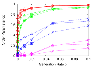
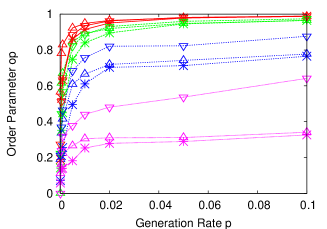
Figure 8: The values of $op$ for the ZRP (top) and Mod 1 (bottom) using n-search. The open $\bigtriangleup$, $\ast$, and $\bigtriangledown$ marks correspond to $\alpha=1.0,0.0$, and $-1.0$, respectively. The red, green, blue, and magenta lines correspond to $\delta=0.0,0.2,0.5$, and $0.8$, respectively.

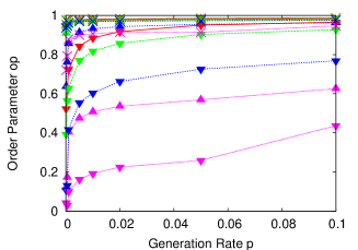
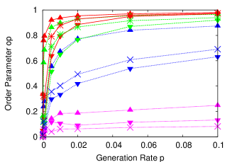
Figure 9: The values of $op$ for Mod 3 (top) and Mod 2 (bottom) at a constant arrival with probability $\mu=0.01$, instead of using n-search. The filled $\bigtriangleup$, $\times$, and $\bigtriangledown$ marks correspond to $\alpha=1.0,0.0$, and $-1.0$, respectively. The red, green, blue, and magenta lines correspond to $\delta=0.0,0.2,0.5$, and $0.8$, respectively.

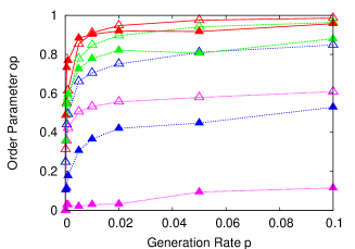
Figure 10: The values of $op$ for a traffic-aware routing Wang06b in which a forwarding node $k$ is chosen by applying Eq.(9) in the cases of n-search (open marks), and of a constant arrival with probability $\mu=0.01$ (filled marks). The red, green, blue, and magenta lines correspond to $\delta=0.0,0.2,0.5$, and $0.8$, respectively.

V Conclusion

For a SF network, whose topology is found in many real systems, we have studied extensions of the ZRP Noh05a ; Noh05b ; Noh07 ; Noh04 which controls both the routing strategies in the preferential Yamashita03 ; Wang06a ; Yan06 and congestion-aware Danila06 walks, and the node performance for packet transfers. Under the assumption of persistent packets, we have approximately analyzed the phase transition between condensation of packets at hubs and uncondensation on SF networks by another straightforward approach Noh05a ; Noh05b instead of the mean-field approximation in the preferential walk for $\alpha>0$ Tang06 . In particular, we have found that uncondensation is maintained in a wide rage of $\delta>\delta_{c}\approx(1+\alpha)/(\gamma-1)$ for $\alpha<0$.

Table 6: Qualitative summary of the traffic properties.

Mean Value	$\alpha>0$	$\alpha<0$	for larger $\delta$
Reachability	low	high	increased $\nearrow$
Num. of Hops	small	large	increased $\nearrow$
Travel Time $\langle T_{a}\rangle$	long	short	decreased $\searrow$
One Wait $\langle T_{w}\rangle/\langle N_{w}\rangle$	long	short	decreased $\searrow$
Num. of Wait $\langle N_{w}\rangle$	small		increased $\nearrow$
		large	decreased $\searrow$
Characteristics	condensation	uniformly
of a Path	at hubs	wandering

Moreover, we have numerically investigated the traffic properties when the practical n-search into a terminal node at the last step takes place. The phase transition has been consistently observed in the cases both with/without n-search. The obtained results are summarized in Table 6. We conclude that the wandering path for $\alpha<0$ better reduces mean travel time of a packet with high reachability in the low-performance regime at a small $\delta$, while in the high-performance regime at a large $\delta$, neither the wandering long path with short wait trapped at nodes ($\alpha=-1$), nor the short hopping path with long wait trapped at hubs ($\alpha=1$) is advisable. A uniformly random walk ($\alpha=0$) yields slightly better performance. This optimality at $\alpha=0$ in a high-performance regime is consistent with the results obtained for the critical generation rate in other traffic model Wang06a on a SF network with node capacity (corresponding to the forwarding performance) proportional to its degree. However, in the details for our traffic model, the optimal case depends on a combination of the values of $\alpha$ and $\delta$ related to the condensation transition at $\delta_{c}$. We emphasize that, for high reachability, small number of hops, and short travel or wait time, such traffic properties summarized in Table 6 as the trade-off between a detour wandering path and long wait at hubs cannot be obtained from only the theoretically predicted phase transition between condensation and uncondensation in Ref. Noh05a ; Noh05b ; Noh07 ; Tang06 . Concerning the fundamental traffic properties, we have investigated the congestion phenomenon with packet generation, compared with other models related to the traffic-aware routing Wang06b ; Echenique05 ; Martino09 . We suggest that the high-forwarding performance at a large $\delta$ is more dominant than the refusal process in order to suppress congestion in a small $op$, and that the difference of $op$ is small when the values of $\alpha$ are varied (the case of $\alpha=0$ is slightly better for n-search). The above results only show qualitative tendencies. In further research, more complex and quantitative properties should be carefully discussed for many combinations of parameters $\alpha$, $\delta$, $\mu$, $\bar{\eta}$, $m^{*}$, etc., although such simulations may be intractable due to huge computation load and memory consumption for the processing of millions of packets in very long iterations.

This direction of research on stochastic routing may be the first step to reveal complex traffic dynamics such as the trade-off between the selection of a short path and long wait (delay) at some particular nodes related to the underlying network structure. We will investigate this problem, including the effects of more realistic selections of the source and the terminal nodes which depend on geographical positions or population density, the queue discipline such as FIFO or LIFO, and other topologies to develop the optimal routing schemes Tadic07 for advanced sensor or ad hoc networks.

*

Appendix A

As a modification to Refs. Noh05a ; Noh05b , we briefly review the derivation of the results presented in Table 3.

For $\delta=0$: case (D), we have a constant jumping rate $q_{i}(\omega)=1$ independent of the occupation number $\omega$ and $F_{i}(z)=\sum_{\omega}\left(zK_{i}^{\beta}\right)^{\omega}=\frac{1}{1-zK_{i}^{\beta}}$. Then, from Eq. (7),

$$m_{K_{i}}=\frac{zK_{i}^{\beta}}{1-zK_{i}^{\beta}}\rightarrow\frac{K_{i}^{\beta}}{K_{max}^{\beta}-K_{i}^{\beta}},$$

is divergent for the hub with the maximum degree $K_{max}$ as $z$ approaches $z_{c}=1/K_{max}^{\beta}$ in the range $z<z_{c}$, because the denominator becomes zero in the first term of the right-hand side, equivalently to the case in which node $i$ has the maximum degree in the second term. It is convenient to decompose the density into two terms such that $\rho=\rho_{s}+\rho_{n}$ for the hub with the maximum degree and for the other nodes. These two terms are given by

$$\rho_{s}=\frac{m_{hub}}{N}=\frac{1}{N}\frac{zK_{max}^{\beta}}{1-zK_{max}^{\beta}},$$ (10)

$$\rho_{n}=\int_{K_{min}}^{K_{max}-1}\frac{zK^{\beta}}{1-zK^{\beta}}P(K)dK.$$ (11)

By using the relation $\frac{1}{1-x}=\sum_{l=0}^{\infty}x^{l}$ for Eq. (11), we derive

$$\begin{array}[]{ll}\rho_{n}&=\int\frac{zK^{\beta}}{1-zK^{\beta}}P(K)dK\\ &=\int zK^{\beta}\sum_{l=0}^{\infty}(zK^{\beta})^{l}P(K)dK\\ &\sim\sum_{l=1}^{\infty}\left\{\int(zK^{\beta})^{l}K^{-\gamma}dK\right\}\\ &=\sum_{l=1}^{\infty}\left\{z^{l}\int K^{\beta l-\gamma}dK\right\}\\ &=\sum_{l=1}^{\infty}\left\{z^{l}\frac{(K_{max}-1)^{(\beta l-\gamma+1)}}{\beta l-\gamma+1}\right\}\\ &\sim\sum_{l=1}^{\infty}\left\{\frac{(zK_{max}^{\beta})^{l}\times(K_{max}^{(-\gamma+1)})}{\beta l}\right\}\\ &=\frac{K_{max}^{(-\gamma+1)}}{\beta}\times\sum_{l=1}^{\infty}\frac{(zK_{max}^{\beta})^{l}}{l}\\ &=\frac{K_{max}^{(-\gamma+1)}}{\beta}\times[-\ln(1-zK_{max}^{\beta})]\\ &\sim N^{-1}\times\ln(1+m_{hub})\rightarrow 0,\end{array}$$

for a large size $N\rightarrow\infty$. In the last terms, we apply $K_{max}^{(-\gamma+1)}\sim N^{-1}$ from $\int_{K_{max}}^{\infty}P(K)dK\sim 1/N$, and

$$\ln\frac{1}{1-x}=-\ln(1-x)=\sum_{l=1}^{\infty}\frac{x^{l}}{l},$$

$$\frac{1}{1-zK_{max}^{\beta}}=1+\rho_{s}N=1+m_{hub}>0,$$

from Eq. (10). Since only $\rho_{s}$ remains, condensation occurs at the hub for any $\alpha$ in case (D) at this uniform jumping rate given by $\delta=0$.

In the general case where $\delta>0$, the infinite series in Eq. (8) does not have a closed form, except for $F_{i}(z)=e^{zK_{i}^{\beta}}$ at $\delta=1$. We approximate the series as in Noh05a ; Noh05b ,

$$F_{i}(z)\approx\frac{1}{\sqrt{\delta}}(2\pi(zK_{i}^{\beta})^{1/\delta})^{(1-\delta)/2}\times\exp(\delta(zK_{i}^{\beta})^{1/\delta}).$$

The second term in the right-hand side is dominant for $zK_{i}^{\beta}\geq 1$. We can simply approximate it with a few lowest-order terms such as $F_{i}(z)=1+zK_{i}^{\beta}+O((zK_{i}^{\beta})^{2})$ for $zK_{i}^{\beta}\ll 1$.

From Eq. (7) and $\partial\ln F_{i}(z)/\partial z$ for the above two cases of $F_{i}(z)$, the mean occupation number is given by

$$m_{K_{i}}\approx\left\{\begin{array}[]{lll}zK_{i}^{\beta}&for&zK_{i}^{\beta}\ll 1\\ (zK_{i}^{\beta})^{1/\delta}&for&zK_{i}^{\beta}\geq 1.\end{array}\right.$$

Thus, the mean occupation number of a node increases monotonically with its degree. Depending on a constant magnitude of $z$, we consider the following two cases (i) and (ii).

(i) We assume that the fugacity $z$ is in such a range that $zK_{i}^{\beta}\geq 1$ for all nodes. From $m_{K_{i}}=(zK_{i}^{\beta})^{1/\delta}$ for all nodes and the self-consistent equation $\rho=\frac{1}{N}\sum_{i}m_{K_{i}}=\frac{1}{N}z^{1/\delta}\sum_{i}(K_{i}^{\beta})^{1/\delta}$, the solution $z=\rho^{\delta}/(\bar{K}^{\beta/\delta})^{\delta}$ is valid only when $\bar{K}^{\beta/\delta}\stackrel{{\scriptstyle\rm def}}{{=}}\int_{K_{min}}^{K_{max}}K^{\beta/\delta}P(K)dK$ remains finite in the limit of large $N$. By using $P(K)\sim K^{-\gamma}$, at $N\rightarrow\infty$, we have

$$\int_{K_{min}}^{K_{max}}K^{\beta/\delta}P(K)dK\sim\int K^{\beta/\delta-\gamma}dK\rightarrow K_{max}^{(\beta/\delta-\gamma+1)}.$$

From the negative exponent, this finite condition imposes that $\delta>\delta_{c}$ with

$$\delta_{c}\stackrel{{\scriptstyle\rm def}}{{=}}\frac{\beta}{\gamma-1}.$$

In this regime, we find $m_{K_{i}}\sim K_{i}^{\beta/\delta}$ for all nodes. The occupation number at the hub with the maximum degree $K_{max}\sim N^{1/(\gamma-1)}$ scales sublinearly as $m_{hub}\sim N^{\beta/\delta(\gamma-1)}=N^{\delta_{c}/\delta}$ with the exponent $\beta/\delta(\gamma-1)=\delta_{c}/\delta<1$. Therefore, the extreme condensation of almost all packets at the hub with $K_{max}$ is avoided when $\delta>\delta_{c}$: case (A).

(ii) We assume that the fugacity $z$ is defined as $K_{c}^{\beta}=1/z$ in the interval $K_{min}<K_{c}<K_{max}$. Then, the self-consistent equation becomes $\rho=\rho_{n}+\rho_{s}=\sum_{i}m_{K_{i}}$, where

$$\rho_{n}=\sum_{K_{min}}^{K_{c}}zK^{\beta}=K_{c}^{-\beta}\int_{K_{min}}^{K_{c}}K^{\beta}P(K)dK,$$ (12)

is the density for the nodes with $K<K_{c}$: $zK^{\beta}<1$, and

$$\rho_{s}=\sum_{K_{c}}^{K_{max}}(zK^{\beta})^{1/\delta}=K_{c}^{-\beta/\delta}\int_{K_{c}}^{K_{max}}K^{\beta/\delta}P(K)dK,$$ (13)

is the density for the nodes with $K>K_{c}$: $zK^{\beta}>1$. Since the integral part in Eq. (12) is smaller than the average $\beta$-power of the degree, $\rho_{n}$ vanishes as $K_{c}^{-\beta}$ in the limit of large $N$. In order to have a finite value of $\rho_{s}=\rho$, the integral part in Eq. (13) should be divergent, which yields that $\delta\leq\delta_{c}=\beta/(\gamma-1)$. This integral should be of the same order as $K_{c}^{-\beta/\delta}$, which yields

$$K_{c}\sim\left\{\begin{array}[]{lll}(\ln K_{max})^{\delta_{c}/\beta}&for&\delta=\delta_{c}\\ (K_{max})^{1-\delta/\delta_{c}}&for&\delta<\delta_{c}.\end{array}\right.$$

in cases (B) and (C), respectively.

References

- (1) R. Albert, and A.-L. Barabási, “Statistical mechanics of complex networks,” Rev. Mod. Phys. Vol. 74, pp. 47, 2002.
- (2) K.-I. Goh, B. Kahng, and D. Kim, “Universal Behavior of Load Distribution in Scale-Free Networks,” Phys. Rev. Lett. Vol. 87, pp. 278701, 2001.
- (3) J. Urrutia, In Handbook of Wireless Networks and Mobile Computing, edited by I. Stojmenović, Chap. 18, John Wiley & Sons, 2002.
- (4) Z. Liu, W, Ma, H. Zhang, Y. Sun, and P. M. Hui, “An efficient approach of controlling traffic congestion in scale-free networks,” Physica A Vol. 370, pp. 843, 2006.
- (5) L. Zhao, Y.-C. Lai, K. Park, and N. Ye, “Onset of traffic congestion in complex networks,” Phys. Rev. E Vol. 71, pp. 026125, 2005.
- (6) J. D. Noh, G. M. Shim, and H. Lee, “Complete Condensation in a Zero Range Process on Scale-Free Networks,” Phys. Rev. Lett. Vol. 94, pp. 198701, 2005.
- (7) J.D. Noh, “Stationary and dynamical properties of a zero-range process on scale-free networks,” Phys. Rev. E Vol. 72, pp. 056123, 2005.
- (8) D. De Martino, L. Dall’Asta, G. Bianconi, and M. Marsili, “Congestion phenomena on complex networks,” Phys. Rev. E Vol. 79, pp. 015101(R), 2009.
- (9) S. Ikeda, I. Kubo, N. Okumoto, and M. Yamashita, “ Impact of Local Topological Information on Random Walks on Finite Graphs,” Lecture Notes in Computer Science Vol. 2719, pp. 1054–1067, 2003.
- (10) W.-X. Wang, B.-H. Wang, C.-Y. Yin, Y.-B. Xie, and T. Zhou, “Traffic dynamics based on local routing protocol on a scale-free network,” Phys. Rev. E Vol. 73, pp. 026111, 2006.
- (11) G. Yan, T. Zhou, B. Hu, Z.-Q. Fu, and B.-H. Wang, “Efficient routing on complex networks,” Phys. Rev. E Vol. 73, pp. 046108, 2006.
- (12) B. Danila, Y. Yu, S. Earl, J. A. Marsh, Z. Toroczkai, and K. E. Bassler, “Congestion-gradient driven transport on complex networks,” Phys. Rev. E Vol. 74, pp. 046114, 2006.
- (13) W.-X. Wang, C.-Y. Yin, G. Yan, and B.-H. Wang, “Integrating local static and dynamic information for routing traffic,” Phys. Rev. E Vol. 74, pp. 016101, 2006.
- (14) P. Echenique, J. Gómez-Gardeñes, and Y. Moreno, “Dynamics of jamming transitions in complex networks,” Eupophys. Lett. Vol. 71, pp. 325, 2005.
- (15) J.D. Noh, “Interacting Particle Systems in Complex Networks,” arXiv:cond-mat/0701401, 2007.
- (16) M. Tang, Z. Liu. and J. Zhou, “Condensation in a zero range process on weighted scale-free networks,” Phys. Rev. E Vol. 74, pp. 036101, 2006.
- (17) A. E. Motter, and Y.-C. Lai, “Cascade-based attacks on complex networks,” Phy. Rev. E Vol. 66, pp. 065102, 2002.
- (18) A. E. Motter, “Cascade Control and Defense in Complex Networks,” Phy. Rev. Lett. Vol. 93, pp. 098701, 2004.
- (19) J. J. Wu, Z. Y. Gao, and H. J.Sun, “Effects of the cascading failures on scale-free traffic networks,” Physica A Vol. 378, pp. 505–511, 2007.
- (20) J. D. Noh, and H. Rieger, “Random Walks on Complex Networks,” Phys. Rev. Lett. Vol. 92, No. 11, pp. 118701, 2004.
- (21) M. R. Evans, “Phase Transitions in one-dimensional nonequilibrum systems,” J. Phys. Vol. 30, pp. 42, 2000.
- (22) B. Tadic, G. J. Rodgers, and S. Thurner, “Transport on Complex Networks: Flow, Jamming & Optimization,” Int. J. Bifurcation and Chaos Vol. 17, No. 7, pp. 2363–2385, 2007.
*