Effect of viscosity and surface tension on the growth of Rayleigh -Taylor instability and Richtmyer-Meshkov instability induced two fluid interfacial nonlinear structure

Abstract

The effect of viscous drag and surface tension on the nonlinear two fluid interfacial structures induced by Rayleigh -Taylor instability and Richtmyer-Meshkov instability are investigated.Viscosity and surface tension play important roles on the fluid instabilities. It is seen that the magnitude of the suppression of the terminal growth rate of the tip of the bubble height depends only on the viscous coefficient of the upper (denser) fluid through which the bubble rises and surface tension of the interface. However, in regard to spike it is shown that in an inviscid fluid spike does not remain terminal but approaches like a free fall under gravity as the Atwood number $(A)$ increases. In this respect there exits qualitative agreement of our results with simulation result as also with some earlier theoretical results. Viscosity reduces the free fall velocity appreciably and it becomes terminal with increasing viscosity. Results obtained from numerical integration of the relevant nonlinear equations describing the temporal development of the spike support the foregoing observations.

Keywords: Shock waves; Gravitational force; Viscosity; Surface tension; Rayleigh-Taylor instability; Richtmyer-Meshkov instability;Bubbles;Spikes
PACS: 52.57Fg,52.57Bc,52.35Tc,51.20+d

I INTRODUCTION

There are many causes for instability of the interface between two fluids. Under the gravitational force when a denser fluid overlies a lighter fluid, the instability occurs and it is called Rayleigh-Taylor instability(RTI). Ritchmeyer-Meshkov instability(RMI) is another type of instability which occurs whenever a shock front crosses the interface of two materials of different shock impendence (the shock must enter from the low independence interface side). Both these instabilities play important role in the ablation region at compression front during the process of inertial confinement fusion, supernova remnant formation or shock tube experiments in the laboratory[1]. In the nonlinear regime the fluid interface forms a finger shape structure.The structure is called a bubble (spike) if the lighter (denser) fluid penetrates into the denser (lighter) fluid. Under astrophysical conditions such structures may cover enormous range of spatial distribution. Examples are suggested to be provided by pillars (”elephant trunk”) of Eagle Nebula which is identified with the spike of a heavy fluid penetrating a lighter fluid[2-5]. Also sudden increase in the height of the ionospheric $F_{2}$ layer is caused by RTI mechanism as suggested by some observational data[6]. Layzer[7] was first to describe the bubble formation in a potential flow model. This model which is based on an approximate description of the flow near the bubble tip describes its nonlinear growth[8-13,26-28].

The effect of viscosity on Rayleigh-Taylor instability and Richtmyer-Meshkov instability shows significant importance for increasing wave number $k$ as $\nu k^{2}$ where $\nu$ is the kinematic coefficient of viscosity.This effect is further enhanced as $\nu$ increase with the temperature for a plasma[14]. The importance of this feature has been discussed for supernova remnant in Ref.[15]. In the domain of linear theory, the effect of viscosity and surface tension on RTI was described in depth by Chandrasekhar [16]. The same effect was described by Mikaelian[17-18] for RMI and for RTI in finite thickness[19]. Higher magnitude of the growth rate suppression due to viscosity was obtained in the weakly nonlinear theoretical study of Carles and Popinet[20]. Later, a time dependent expression of the reduced linear theory growth rate of RTI and RMI due to the combined effect of viscosity and binary mass diffusivity between the fluids was arrived at in linear theory by Robey[21]. The effect of surface tension under the weakly nonlinear theory was analyzed by Garnier et al.[22] and later Roy et al.[29] studied the same effect in nonlinear theory.

The present paper reports the combined effect of viscosity and surface tension on the two fluid nonlinear interfacial finger like structures resulting due to RTI and RMI. We have analyzed the problem based on Layzer’s approach. It is seen that, in absence of surface tension the lowering of the asymptotic velocity of the tip of the bubble which is formed when the lighter (the lower) fluid penetrates into the denser (the upper) fluid and thus encounters the viscous drag due to the denser fluid,depends only on the viscosity coefficient of denser fluid. However, in presence of surface tension, the asymptotic velocity of the tip of the bubble and nonlinear perturbed surface are oscillating under certain conditions. It has been shown that, for RTI this oscillation depends only on the surface tension but for RMI it depends on surface tension as well as viscosity.

On the other hand it is shown that in an inviscid fluid the spikes do not remain terminal as obtained in theoretical works[10,13]. It is only discussed in ref.9 that the RTI spike was shown to have a free fall $\sim\frac{1}{2}gt^{2}$ where $g$ is acceleration due to gravity and the RMI spike to have a constant velocity of fall but that too only for Atwood number $A=1$. In the present analysis the free fall behavior is seen to hold for all values of Atwood number $A$. The depth of the tip of the spike below the unperturbed interfacial surface is $\sim\frac{1}{2}\gamma gt^{2}$ where $\gamma$ is a dimensionless constant which $\rightarrow 1$ as $A\rightarrow 1$. Similar result is found to hold for RMI. The effect of viscosity is seen to reduce the spike velocity appreciably and as the viscosity coefficient increases the spike velocity tends to become approximately terminal. Such behavior of both RTI and RMI spike for for inviscid and viscous fluids was not found earlier.

The paper is organized as follows: In Section II, we describe the basic fluid equation with the assumption that the motion is irrotational and fluid is incompressible. Also the kinematic and dynamical boundary condition are derived in Sec.II. The analytical expressions of the viscosity and surface tension induced asymptotic velocity of the tip of the bubble and associated numerical results are given in Section III. Section IV is devoted to temporal development of the spike. The results are summarized in Section V.

II BASIC EQUATION AND BOUNDARY CONDITIONS

The $x-y$ plane ($z=0$) is assumed to be the unperturbed interface between the denser fluid of density $\rho_{h}$ (region $z>0$) and lighter fluid of density $\rho_{l}$ (region $z<0$). The variables with subscript $h$ and $l$ represents denser and lighter fluid, respectively. Gravity $g$ is taken to point along negative $z$-axis. After perturbation the finger shape interface is assumed to take up a parabolic form, given by

$$z=\eta(x,t)=\eta_{0}(t)+\eta_{2}(t)x^{2}$$ (1)

$$\mbox{For a bubble:}\qquad\qquad\eta_{0}>0\quad\mbox{and}\quad\eta_{2}<0,$$ (2)

$$\mbox{For a spike:}\qquad\qquad\eta_{0}<0\quad\mbox{and}\quad\eta_{2}>0.$$ (3)

Following Goncharov [13], the velocity potentials describing the irrotational motion for the denser and lighter fluids are assumed to be given by

$$\phi_{h}(x,z,t)=a_{1}(t)\cos{(kx)}e^{-k(z-\eta_{0}(t))};\quad z>0$$ (4)

$$\phi_{l}(x,z,t)=b_{0}(t)z+b_{1}(t)\cos{(kx)}e^{k(z-\eta_{0}(t))};\quad z<0$$ (5)

where $k$ is the perturbed wave number.

To find the five unknown functions i.e. $\eta_{0}(t)$,$\eta_{1}(t)$,$a_{1}(t)$,$b_{0}(t)$ and $b_{1}(t)$, we require as many equations obtained from the kinematical and dynamical boundary conditions describing the dynamics.

We first turn to the kinematical boundary conditions corresponding to the interfacial surface perturbations represented by eq.(1):

$$\eta_{x}(v_{h})_{x}-\eta_{x}(v_{l})_{x}=(v_{h})_{z}-(v_{l})_{z}$$ (6)

$$\eta_{t}+\eta_{x}(v_{h})_{x}=(v_{h})_{z}$$ (7)

Substituting eq.(6) and eq.(7)from eq.(1) and for $(v_{h(l)})_{x}=-\frac{\partial\phi_{h(l)}}{\partial x}$ and $(v_{h(l)})_{x}=-\frac{\partial\phi_{h(l)}}{\partial x}$ from eq.(4)and eq.(5) and expanding in powers of the transverse coordinate $x$ neglecting terms O($x^{i}$)($i\geq 3$), we obtain the following relations which are equivalent to the kinematic boundary conditions eq.(6) and eq.(7):

$$\frac{d\xi_{1}}{d\ t}=\xi_{3}$$ (8)

$$\frac{d\xi_{2}}{d\ t}=-\frac{1}{2}(6\xi_{2}+1)\xi_{3}$$ (9)

$$b_{0}=-\frac{6\xi_{2}}{3\xi_{2}-\frac{1}{2}}ka_{1}$$ (10)

$$b_{1}=\frac{3\xi_{2}+\frac{1}{2}}{3\xi_{2}-\frac{1}{2}}a_{1}$$ (11)

$$\mbox{where }\xi_{1}=k\eta_{0};\qquad\xi_{2}=\eta_{2}/k;\qquad\xi_{3}=k^{2}a_{1};\qquad\tau=t\sqrt{kg}$$ (12)

$\xi_{1}$ and $\xi_{2}$ are, respectively, the non-dimensionalized displacement and curvature at the tip of the nonlinear structure, $\xi_{3}/k$ is its velocity and $\tau$ is the non-dimensionalized time. Eq.(8) and eq.(9) are the first two of the three time development equations needed to describe the time evaluation of the nonlinear structure (the other two viz $b_{0}(t)$ and $b_{1}(t)$ are provided by eq.(10) and eq.(11)) .

For the constant density fluid, the equation of continuity is $\vec{\nabla}.\vec{v}=0$, which becomes $\nabla^{2}\phi=0$ for potential flow. So, for a fluid with uniform viscosity having coefficient of viscosity $\mu_{h(l)}$, the viscous term drops out ($\mu\nabla^{2}\vec{v}=\mu\vec{\nabla}(\nabla^{2}\phi)=0$) in

$$\rho\left[\frac{\partial\vec{v}}{\partial t}+(\vec{v}.\vec{\nabla})\vec{v}\right]=-\vec{\nabla}p+\mu\nabla^{2}\vec{v}-\rho g\hat{z}$$ (13)

and we arrive at the first integral of the momentum equation.

$$-\rho_{h(l)}\frac{\partial\phi_{h(l)}}{\partial t}+\frac{1}{2}\rho_{h(l)}(\vec{\nabla}\phi_{h(l)})^{2}+\rho_{h(l)}gz=-p_{h(l)}+f_{h(l)}(t)$$ (14)

The net stress [16] at two fluid interface including that due to viscosity is

$$P_{h(l)}=-p_{h(l)}+2\mu_{h(l)}\frac{\partial(v_{h(l)})_{z}}{\partial t}$$ (15)

Plugging the dynamical boundary condition $P_{h}-P_{l}=-T/R$ at the interface $z(x,t)=\eta(x,t)$, where $R$ is the radius of curvature and $T$ is the surface tension of the perturbed interface, in eq.(14) and eq.(15) we obtained the following equation[23].

$$\rho_{h}[-\frac{\partial\phi_{h}}{\partial t}+\frac{1}{2}(\vec{\nabla}\phi_{h})^{2}]-\rho_{l}[-\frac{\partial\phi_{l}}{\partial t}+\frac{1}{2}(\vec{\nabla}\phi_{l})^{2}]+g(\rho_{h}-\rho_{l})z=2[\mu_{h}\frac{\partial^{2}\phi_{h}}{\partial z^{2}}-\mu_{l}\frac{\partial^{2}\phi_{l}}{\partial z^{2}}]-\frac{T}{R}+f_{h}-f_{l}$$ (16)

at the interface $z(x,t)=\eta(x,t)$.

Substituting for $\phi_{h}$,$\phi_{l}$ from eq.(4),eq.(5) and value of $\frac{1}{R}$, using eq.(10)-eq.(12) and equating coefficient of $x^{2}$, we obtain after some straightforward but lengthy algebraic manipulation, the following time development equation for $\xi_{3}$:

$$\frac{d(\xi_{3}/\sqrt{kg})}{d\tau}=-\frac{N(\xi_{2},r)}{D(\xi_{2},r)}\frac{(\xi_{3}/\sqrt{kg})^{2}}{(6\xi_{2}-1)}+2(r-1)\frac{\xi_{2}(6\xi_{2}-1)}{D(\xi_{2},r)}(1-12\xi_{2}^{2}\frac{k^{2}}{k_{c}^{2}})$$

$$-\frac{2(\xi_{3}/\sqrt{kg})}{D(\xi_{2},r)}rc_{h}[(s+1)(1-12\xi_{2}^{2})+4\xi_{2}(s-1)]\hskip 50.0pt$$ (17)

where

$$\quad r=\frac{\rho_{h}}{\rho_{l}};\nu_{h(l)}=\frac{\mu_{h(l)}}{\rho_{h(l)}};s=\frac{\mu_{l}}{\mu_{h}};c_{h}=\frac{k^{2}\nu_{h}}{\sqrt{kg}};k_{c}^{2}=\frac{(\rho_{h}-\rho_{l})g}{T}$$ (18)

$$D(\xi_{2},r)=12(1-r)\xi_{2}^{2}+4(1-r)\xi_{2}+(r+1);$$

$$N(\xi_{2},r)=36(1-r)\xi_{2}^{2}+12(4+r)\xi_{2}+(7-r)$$ (19)

Eq.(8) and eq.(9) together with eq.(17) governs the temporal development of the Rayleigh-Taylor instability. For Richtmyer-Meshkov instability, the gravity dependent term in eq.(17) vanishes i.e. $g=0$ and the equation for $\frac{d\xi_{3}}{dt}$ becomes

$$\frac{d(\xi_{3}/\sqrt{kg})}{d\tau}=-\frac{N(\xi_{2},r)}{D(\xi_{2},r)}\frac{(\xi_{3}/\sqrt{kg})^{2}}{(6\xi_{2}-1)}-\frac{24(r-1)\xi_{2}^{3}(6\xi_{2}-1)}{D(\xi_{2},r)}\frac{k^{2}}{k_{c}^{2}}$$

$$-\frac{2(\xi_{3}/\sqrt{kg})}{D(\xi_{2},r)}rc_{h}[(s+1)(1-12\xi_{2}^{2})+4\xi_{2}(s-1)]\hskip 1.0pt$$ (20)

III SUPPRESSION AND OSCILLATION OF ASYMPTOTIC BUBBLE VELOCITY

The nondimensionalized time development plots of $\xi_{1}$,$\xi_{2}$ and $\xi_{3}$ for RTI bubble are shown in Figure 1. As $\tau\rightarrow\infty$, the asymptotic values of $\xi_{2}$ and $\xi_{3}$ for bubble are obtained by setting $\frac{d\xi_{2}}{d\tau}=0$ giving $[(\xi_{2})_{asymp}]_{bubble}=-\frac{1}{6}$ and $\frac{d(\frac{\xi_{3}}{\sqrt{kg}})}{d\tau}=0$ yielding

$$[(\xi_{3})_{asymp}]_{bubble}=\frac{\frac{2}{3}\frac{A}{1+A}kg(1-\frac{k^{2}}{3k_{c}^{2}})}{\sqrt{\frac{4}{9}{\nu_{h}}^{2}k^{4}+\frac{2}{3}\frac{A}{(1+A)}kg(1-\frac{k^{2}}{3k_{c}^{2}})}+\frac{2}{3}\nu_{h}k^{2}}$$ (21)

It is interesting to note that if $k^{2}<3k_{c}^{3}$, the asymptotic velocity of the bubble caused by the rising of the lighter (lower) fluid also by pushing through the denser (upper) fluid is affected only by the viscous drag exerted by the later.This is clearly seen from eq.(21) as $[(\xi_{3})_{asymp}]_{bubble}$ depends only on the kinematic viscosity of the denser (upper) fluid ($\nu_{h}$,). If $k^{2}=3k_{c}^{2}$ equilibrium is attained; but if $k^{2}>3k_{c}^{2}$, this reverse the sign of the second term in eq.(17) leads to the emergence of oscillatory state (Figure 2).

Similar results for temporal development of Richtmyer-Meshkov instability are shown in Figure 3. The asymptotic velocity is

$$[(\xi_{3})_{asymp}]_{bubble}=-\frac{2k^{2}\nu_{h}}{3}+\sqrt{\frac{4}{9}\nu_{h}^{2}k^{4}-kg\frac{2A}{9(1+A)}\frac{k^{2}}{k_{c}^{2}}}\coth{[(\frac{3(1+A)}{3+A}\sqrt{\frac{4}{9}\nu_{h}^{2}k^{4}-kg\frac{2A}{9(1+A)}\frac{k^{2}}{k_{c}^{2}}})t]}$$ (22)

For bubble as well as for spike, $[(\xi_{3})_{asymp}]_{bubble}\rightarrow-\frac{2k^{2}\nu_{h}}{3}+\sqrt{\frac{4}{9}\nu_{h}^{2}k^{4}-kg\frac{2A}{9(1+A)}\frac{k^{2}}{k_{c}^{2}}}$ exponentially with time. In absence of surface tension the time dependence is qualitatively similar to that for linear theoretical result of Mikaelian[17] but with different Atwoood number and kinematic viscosity coefficient dependence. However, the weakly nonlinear theoretical results of Carles and Popinet[20] shows a different time dependence $~{}a[1-\frac{4}{3\sqrt{\pi}}k\sqrt{\nu t}]$. On the other hand in case of RMI,for $k^{2}>2c_{h(l)}^{2}k_{c}^{2}\frac{1+A}{A}$ the asymptotic velocity of the bubble as well as the perturbed surface elevation oscillates. This is represented in Figure 4.

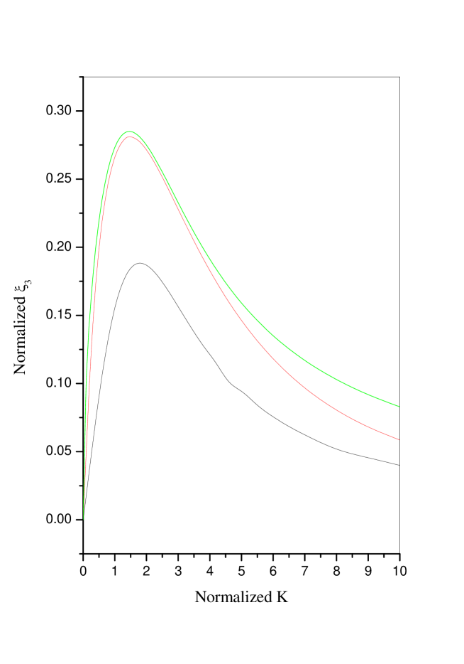
Figure 5: Variation of normalize $\xi_{3}$ with normalize ’k’ for RTI bubble with $c_{h}=0.1$, $r=1.5$, $\frac{k^{2}}{k_{c}^{2}}$= 0 and $\tau=$ 3(Black), 8(Red), $\infty$ (Green).

In absence of surface tension both RTI and RMI are characterized by linear inviscid growth rate which increase with increasing wave number $k$. The dissipative effect due to viscosity also increases with increasing $k$ and suppress the growth rate. A graphical representation of the wave number dependence of the nonlinear growth rate of the hight of the tip of the bubble is shown in Figure 5. The nature of $k-$ dependence is qualitatively similar to that in linear case [21] except that for $t\rightarrow\infty$ where the growth rate tends to a saturation value for all $k$ in the nonlinear case.For bubble the asymptotic growth rate for RTI is maximum at $[k_{max}]_{bubble}=\sqrt[3]{\frac{3A}{16(1+A)}\frac{g}{\nu_{h}^{2}}}$.

Thus for RTI the growth rate and perturbed interface are oscillating due to surface tension while for RMI oscillation depends on the relative strength of surface tension and viscous drag.

IV TIME DEVELOPMENT OF SPIKE

To study the time evolution of spikes we adopt a procedure different from the usual Goncharov transformation[13]. We cast time evolution eq.(17) in the form given bellow.

$$\frac{d(\xi_{3}/\sqrt{kg})}{d\tau}=-\frac{1}{2(\xi_{2}-\frac{1}{6})(\xi_{2}-\beta_{+})(\xi_{2}-\beta_{-})}[(\xi_{2}-\alpha_{+})(\xi_{2}-\alpha_{-})(\xi_{3}/\sqrt{kg})^{2}+2\xi_{2}(\xi_{2}-\frac{1}{6})^{2}(1-12\xi_{2}^{2}\frac{k^{2}}{k_{c}^{2}})$$

$$\hskip 73.0pt-\frac{1}{3}(\xi_{2}-\frac{1}{6})rc_{h}[(s+1)(1-12\xi_{2}^{2})+4\xi_{2}(s-1)](\xi_{3}/\sqrt{kg})]$$ (23)

by using the following expression for $N(\xi_{2},r)$ and $D(\xi_{2},r)$:

$$N(\xi_{2},r)=-36(r-1)(\xi_{2}-\alpha_{+})(\xi_{2}-\alpha_{-})$$

$$D(\xi_{2},r)=-12(r-1)(\xi_{2}-\beta_{+})(\xi_{2}-\beta_{-})$$ (24)

$$\mbox{where }\alpha_{\pm}=\frac{(r+4)\pm\sqrt{16r+4}}{6(r-1)}$$

$$\beta_{\pm}=\frac{-1\pm\sqrt{\frac{4r+2}{r-1}}}{6}\hskip 35.0pt$$ (25)

Clearly $\alpha_{+}>\alpha_{-}$ and $\beta_{+}>\beta_{-}$ and also $\alpha_{+}>\beta_{+}$, $\alpha_{+}>\frac{1}{6}$

First we consider the temporal development of spike as a result of RTI in an inviscid fluid with absence of surface tension, i.e., we put $c_{h}=0$ and $\frac{1}{k_{c}^{2}}=0$ in eq.(17). We start with an initial value of $\xi_{2}=\xi_{20}>\alpha_{+}>\beta_{+}$ and $\frac{1}{6}$, and $\xi_{30}<0$.

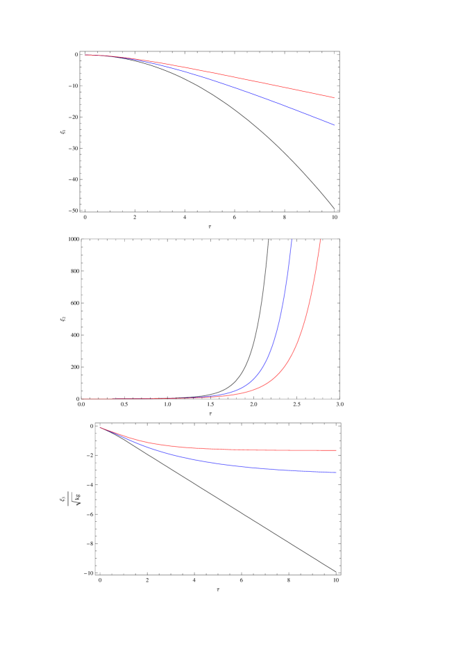
Figure 6: Variation of $\xi_{1}$,$\xi_{2}$ and $\xi_{3}/\sqrt{kg}$ with $\tau$ as obtained by the solution of the eq.(8),eq.(9) and eq.(17) for RTI spike with initial value $\xi_{1}=-0.1$, $\xi_{1}=1$, $\xi_{3}/\sqrt{kg}=-0.1$, $r=5$,$s=1/5$, $\frac{k^{2}}{k_{c}^{2}}=0$ and $c_{h}$= 0.0 (Black), 0.1(Blue), 0.2(Red).

Eq.(9) shows that $\frac{d\xi_{2}}{d\tau}>0$ while eq.(23) shows that $\frac{d(\xi_{3}/\sqrt{kg})}{d\tau}<0$ (as the square bracketed term on the RHS of the latter equation is positive) for all $\tau$ when one starts from such initial values. Thus $\xi_{2}(\tau)$ is a monotonically increasing and $\xi_{3}/\sqrt{kg}$ is a monotonically decreasing function of time $\tau$. Now the curvature at the tip of the spike, i.e., $x=0$ is $\frac{1}{R}=\frac{\partial^{2}\eta}{\partial x^{2}}/[1+(\frac{\partial\eta}{\partial x})^{2}]^{\frac{3}{2}}=2\eta_{2}(\tau)=k\xi_{2}(\tau)$. Thus the curvature of the spike increases with time while the acceleration of the tip of spike $\frac{d(\xi_{3}/\sqrt{kg})}{d\tau}$ (directed downward) tends to a constant value as may be interred from eq.(23) when viscosity and surface tension are neglected. Thus the spike appears to fall continuously and simultaneously gets sharpened. This result is quite different from the earlier results obtained by Goncharov’s transformation which concludes that the spike velocity tends asymptotically to a constant value. Our result is in conformity with expected spike behavior and is in agreement with some earlier theoretical results obtained by a different approximate method[24][25]. The same qualitative spike behavior is exhibited in presence of viscosity but with much reduced speed of fall of the tip of the spike. This is demonstrated in Figure 6 and Figure 7 obtained from the results derived from numerical integration of eq.(8), eq.(9) and eq.(23). Figure 6 shows that the spike speed decreases as the coefficient of viscosity increases. Moreover, for $c_{h}=0$ (inviscid fluid) the spike velocity is seen to vary linearly with time (i.e., close to free fall velocity) so that the displacement of the tip of the spike $\sim\frac{1}{2}\gamma gt^{2}$ where $\gamma$ is a dimensionless constant and value of $\gamma$ close to unity as $A\rightarrow 1$.

Rayleigh-Taylor instability is driven by gravity $g$ while Richtmyer-Meshkov instability is switched on by the impingement of a shock which impulsively changes the normal velocity by the amount $\Delta v=v_{after}-v_{before}$. Thus Richtmyer-Meshkov instability is driven by the instantaneous acceleration $\triangle v\delta(t)$. This has the consequence that the dynamical variables are to be nondimensionalized using normalization in terms of $(k\triangle v)$ for RMI instead of $\sqrt{kg}$ for RTI. Hence, in RMI equations $\frac{\xi_{3}}{\sqrt{kg}}$, $c_{h}$ and $\tau$ are replaced by

$$\frac{\xi_{3}}{\sqrt{kg}}=\frac{\xi_{3}}{(k\Delta v)},\mbox{ }\overline{c}_{h}=\frac{k^{2}\nu_{h}}{(k\triangle v)},\mbox{ }\overline{\tau}=t(k\Delta v)$$ (26)

With replacements as gravity by eq.(26), the temporal development of RMI spike growth are obtained from numerical integration of eq.(8), eq.(9) and eq.(23) when the gravity $g$ induced second term in the square bracket on the RHS of the last mentioned equation is to be deleted. The absence of gravity induced acceleration keeps $\frac{\xi_{3}}{(k\Delta v)}$ close to its initial value when viscosity is neglected $(\overline{c}_{h}=0)$ but tends to vanish when $\overline{c}_{h}\neq 0$.

The lowering of the value of $\frac{\xi_{3}}{(k\Delta v)}$ in magnitude will according to eq.(9) reduce the rate of growth of the curvature $\xi_{2}$ with respect to $\overline{\tau}$ (nondimensionalized time). Thus, in contrast to the free fall of RTI spike, the RMI spike tip descends at an almost constant rate. The curvature also increases slowly, i.e, the spike sharpens at a much reduced rate as it falls (as compared to the RTI spike). All these features are shown in figure 8 and figure 9. The growth rate are seen to be further reduced due to the viscous drag.

Finally, we note the difference between the RTI and RMI parabolic spike structures (figure 7 and figure 9) given by

$$ky=k\eta_{0}(t)+(\frac{\eta_{2}(t)}{k})(kx)^{2}$$

$$=\xi_{1}(t)+\xi_{2}(t)(kx)^{2}\hskip 19.0pt$$ (27)

Let us first consider the inviscid case. The discussions in the foregoing paragraphs indicate that

$$\xi_{1}(\tau)\sim-\frac{1}{2}\tau^{2}\mbox{ for RTI while }\xi_{1}(\overline{\tau})\sim-\mbox{(constant) }\overline{\tau}\mbox{ for RMI }$$ (28)

Further from eq.(8) and eq.(9) which gives $(\xi_{2}+\frac{1}{6})=(\xi_{20}+\frac{1}{6})exp[-3(\xi_{1}-\xi_{10})]$ ($\xi_{10}$ and $\xi_{20}$ are initial values) we obtain

$$\xi_{2}(\tau)\sim\mbox{(constant) }\exp[\frac{3}{2}\tau^{2}]\mbox{ for RTI while }\xi_{2}(\overline{\tau})\sim\mbox{ (constant) }\exp[\mbox{ (constant) }\overline{\tau}]\mbox{ for RMI }$$ (29)

Eq.(28) and eq.(29) when plugged in eq.(27), now clearly indicates that the RTI spike fall much faster and gets sharpened much more rapidly. In both cases, the effect of viscosity is to dampen the growth rates. This leads to difference in the RTI and RMI spike structures as seen in figure 7 and figure 9.

V SUMMARY

Finally we briefly summarize the results:
(i) For RTI the asymptotic velocity of the tip of the bubble is given by
$[(\xi_{3})_{asymp}]_{bubble}=$ $\frac{\frac{2}{3}\frac{A}{1+A}kg(1-\frac{k^{2}}{3k_{c}^{2}})}{\sqrt{\frac{4}{9}{\nu_{h}}^{2}k^{4}+\frac{2}{3}\frac{A}{(1+A)}kg(1-\frac{k^{2}}{3k_{c}^{2}})}+\frac{2}{3}\nu_{h}k^{2}}$
and for RMI, the asymptotic velocity of the bubble is given by
$[(\xi_{3})_{asymp}]_{bubble}=-\frac{2k^{2}\nu_{h}}{3}+\sqrt{\frac{4}{9}\nu_{h}^{2}k^{4}-kg\frac{2A}{9(1+A)}\frac{k^{2}}{k_{c}^{2}}}$ $\coth{[(\frac{3(1+A)}{3+A}\sqrt{\frac{4}{9}\nu_{h}^{2}k^{4}-kg\frac{2A}{9(1+A)}\frac{k^{2}}{k_{c}^{2}}})t]}$.

(ii) In case of RTI, if $k^{2}<3k_{c}^{2}$ the asymptotic velocity of the bubble is affected only by the viscous drag of the upper fluid(Figure 1) and similar effect for RMI with $k^{2}<2c_{h}^{2}k_{c}^{2}\frac{1+A}{A}$(Figure 3).

(iii) For RTI, the growth rate and perturbed surface are oscillating if $k^{2}>3k_{c}^{2}$, i.e the oscillation depends only on the surface tension of the perturbed interface (Figure 2) while for RMI the growth rate and perturbed surface are oscillating if $k^{2}>2c_{h}^{2}k_{c}^{2}\frac{1+A}{A}$, i.e the oscillation depends on the surface tension of the perturbed interface as well as the coefficient of viscosity (Figure 4).

(iv) In inviscid fluid the RTI spike has no asymptotically terminal velocity. Rather the spike has a nearly free fall so that the depth of the tip of the spike below unperturbed surface of separation $\sim\frac{1}{2}\gamma gt^{2}$ where $\gamma$ is a dimensionless constant and value of $\gamma$ close to unity as $A\rightarrow 1$; also the spike sharpens as it falls. For viscous fluid the velocity of fall gets reduced as the coefficient of viscosity increases and tends to a nearly terminal velocity for sufficiently large viscosity. Similar result holds for RMI. The results are demonstrated in Figure 8 and Figure 9.

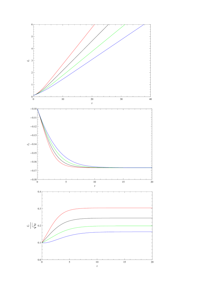
Figure 1: Variation of $\xi_{1}$,$\xi_{2}$ and $\xi_{3}/\sqrt{kg}$ with $\tau$ as obtained by the solution of the eq.(8),eq.(9) and eq.(17) for RTI bubble with initial value $\xi_{1}=0.1$, $\xi_{1}=-0.1$, $\xi_{3}/\sqrt{kg}=0.1$, $r=1.5$, $\frac{k^{2}}{k_{c}^{2}}=0.5$ and $c_{h}$= 0 (Red), 0.1(Black), 0.2(Green), 0.3(Blue).

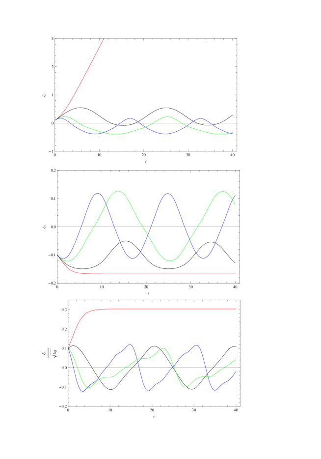
Figure 2: Variation of $\xi_{1}$,$\xi_{2}$ and $\xi_{3}/\sqrt{kg}$ with $\tau$ as obtained by the solution of the eq.(8),eq.(9) and eq.(17) for RTI bubble with initial value $\xi_{1}=0.1$, $\xi_{1}=-0.1$, $\xi_{3}/\sqrt{kg}=0.1$, $r=1.5$, $c_{h}=0.001$ and $\frac{k^{2}}{k_{c}^{2}}$= 0.5 (Red), 5(Black), 10(Green), 15(Blue).

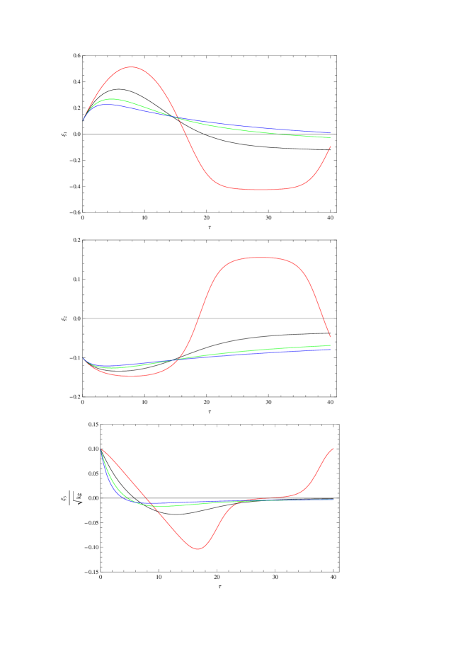
Figure 3: Variation of $\xi_{1}$,$\xi_{2}$ and $\xi_{3}/\sqrt{kg}$ with $\tau$ as obtained by the solution of the eq.(8),eq.(9) and eq.(20) for RMI bubble with initial value $\xi_{1}=0.1$, $\xi_{1}=-0.1$, $\xi_{3}/\sqrt{kg}=0.1$, $r=1.5$, $\frac{k^{2}}{k_{c}^{2}}=0.5$ and $c_{h}$= 0 (Red), 0.1(Black), 0.2(Green), 0.3(Blue).

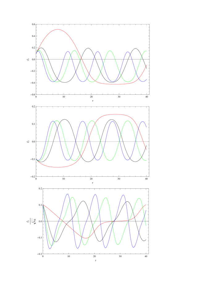
Figure 4: Variation of $\xi_{1}$,$\xi_{2}$ and $\xi_{3}/\sqrt{kg}$ with $\tau$ as obtained by the solution of the eq.(8),eq.(9) and eq.(20) for RMI bubble with initial value $\xi_{1}=0.1$, $\xi_{1}=-0.1$, $\xi_{3}/\sqrt{kg}=0.1$, $r=1.5$, $c_{h}=0.001$ and $\frac{k^{2}}{k_{c}^{2}}$= 0.5 (Red), 5(Black), 10(Green), 15(Blue).

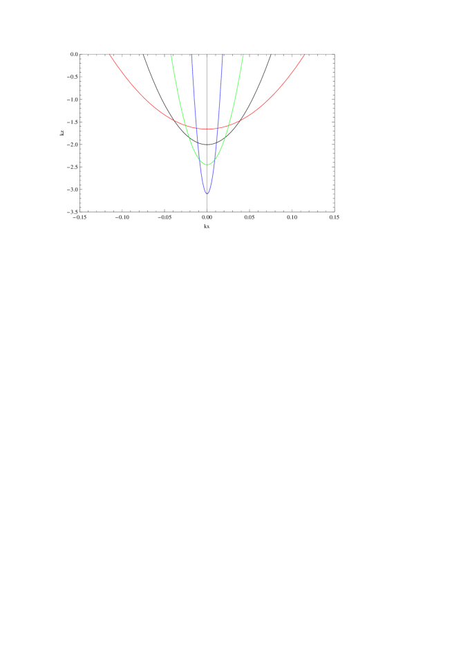
Figure 7: Formation of RTI spike where $r=5$,$s=1/5$, $\frac{k^{2}}{k_{c}^{2}}=0$ and $c_{h}$= 0.0, $\tau=2$(Black), $c_{h}$= 0.0, $\tau=2.5$(Blue), $c_{h}$= 0.1, $\tau=2$(Red), $c_{h}$= 0.1, $\tau=2.5$(Green).

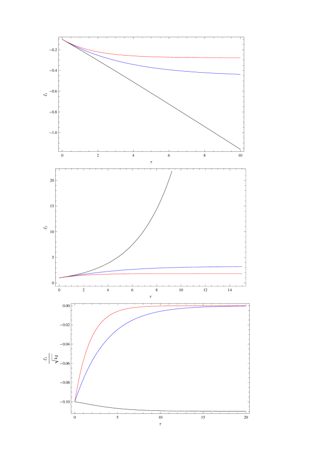
Figure 8: Variation of $\xi_{1}$,$\xi_{2}$ and $\xi_{3}/\sqrt{kg}$ with $\tau$ as obtained by the solution of the eq.(8),eq.(9) and eq.(20) for RMI spike with initial value $\xi_{1}=-0.1$, $\xi_{1}=1$, $\xi_{3}/\sqrt{kg}=-0.1$, $r=5$, $s=1/5$, $\frac{k^{2}}{k_{c}^{2}}=0$ and $c_{h}$= 0.0 (Black), 0.1(Blue), 0.2(Red).

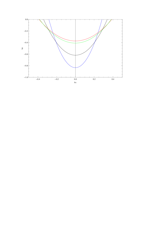
Figure 9: Formation of RMI spike where $r=5$,$s=1/5$, $\frac{k^{2}}{k_{c}^{2}}=0$ and $c_{h}$= 0.0, $\tau=2$(Black), $c_{h}$= 0.0, $\tau=2.5$(Blue), $c_{h}$= 0.1,$\tau=2$(Red), $c_{h}$= 0.1, $\tau=2.5$(Green). RTI and RMI spike structures are different because the RTI is given by the acceleration $g$ while RMI spike induced by shock velocity discuss below eq.(29)

References

- [1] R P Drake High Energy Density Physics Springer, 2006.
- [2] L Spitzar Astrophys. J. 120, 1 (1954).
- [3] E A Frieman Astrophys. J. 120, 18 (1954).
- [4] B A Remington, R P Drake D D Ryutov Rev. Mod. Phys. 78, 755 (2006).
- [5] D D Ryutov, B A Remington Plasma Phys. and Controlled Fusion 44, B407 (2002).
- [6] S S V N Prasad, J V Prasad, N S M P Latadevi P V S Rama Rao Ind. J. Phys. 84, 345 (2010).
- [7] D Layzer Astrophys. J. 122, 1 (1955).
- [8] J Hecht,U Alon,D Shavrts Phys. Fluids 6, 4019 (1994).
- [9] Q Zhang Phys. Rev. Lett. 81, 3391 (1998).
- [10] K O Mikaelian Phys. Rev.Lett. 80, 508 (1998).
- [11] Sung-Ik Sohn Phys. Rev. E 67, 026301 (2003).
- [12] V N Goncharov,D Li Phys. Rev. E 71, 046306 (2005).
- [13] V N Goncharov Phys. Rev. Lett. 88, 134502 (2002).
- [14] L Spitzar Physics of Fully Ionized Gases, (John Wiley and Sons Inc.,NewYork,1962).
- [15] P F Velazquez, D O Gomez, G M Dubner, G G Castro,A Costa, Astron. Astrophys. 334, 1060 (1998).
- [16] S Chandrasekhar Hydrodynamic and Hydromagnetic Stability, (Dover,Newyork,1961).
- [17] K O Mikaelian Phys. Rev. E 47,375 (1993).
- [18] K O Mikaelian Phys. Rev.A 42, 7211 (1990).
- [19] K O Mikaelian Phys. Rev.A 54, 3676 (1996).
- [20] P Carles, S Popinet Phys. Fluids 13, 1833 (2001).
- [21] H F Robey Phys. Plasmas 11, 4123 (2004).
- [22] J Garnier, C Cherfils-Clerouin, A P Holstein Phys. Rev.E 68, 036401 (2003).
- [23] Sung-Ik Sohn Phys. Rev. E 80, 055302(R) (2009).
- [24] P Clavin, F Williams, J. Fluid Mech. 525, 105 (2005).
- [25] L Duchemin, C Josserand, P Clavin, Phys. Rev. Lett. 94, 224501 (2005).
- [26] M R Gupta, L K Mandal, S Roy, M Khan, Phys. Plasmas 17 (2010) 012306 .
- [27] M R Gupta, S Roy, M Khan, H C Pant, S Sarkar, M K Srivastava Phys. Plasmas 16 (2009) 032303 .
- [28] R Banerjee, L Mandal, S Roy, M Khan, M R Gupta Phys. Plasmas 18, 022109 (2011).
- [28] S Roy, M R Gupta, M Khan, H C Pant, M K Srivastava Journal of Phys: Conference Series 208, 012083 (2010).