Bright Chirp-free and Chirped Nonautonomous solitons under Dispersion and Nonlinearity Management

Abstract

We present a series of chirp-free and chirped analytical nonautonomous soliton solutions to the generalized nonlinear Schrödinger equation (NLSE) with distributed coefficients by Darboux transformation from a trivial seed. For chirp-free nonautonomous soliton, the dispersion management term can change the motion of nonautonomous soliton and do not affect its shape at all. Especially, the classical optical soliton can be presented with variable dispersion term and nonlinearity when there is no gain. For chirped nonautonomous soliton, dispersion management can affect the shape and motion of nonautonomous solitons meanwhile. The periodic dispersion term can be used to control its “breathing” shape, and it does not affect the trajectory of nonautonomous soliton center with a certain condition.

Keywords: Bright nonautonomous soliton, Dynamics, Dispersion management

190.0190, 190.5530, 260.2030.

1 Introduction

It is well known that ideal optical soliton in fiber, theoretically reported by Hasegawa and Tappert [1, 2] and experimentally verified by Molenauer et al.[3], is based on the exact balance between the group velocity dispersion and the self-phase modulation. However, it is very difficult to realize ideal optical soliton communication due to fiber loss. The dissipation would weaken the nonlinearity and finally the optical soliton would broaden and lose its signal[4]. There are two ways to overcome these inferiors. One is to compensate for the fiber loss by optical gain via Raman amplification [5]. The other is to use dispersion management and nonlinearity management, which have been investigated in recent years [6] and [7]. When the two techniques are performed, the dynamics of optical pulse propagation will be governed by inhomogeneous nonlinear Schrödinger equation (INLSE)

$$i\frac{\partial U}{\partial Z}+\Omega(Z)\frac{\partial^{2}U}{\partial T^{2}}+R(Z)|U|^{2}U+\frac{iG(Z)}{2}U=0\ ,$$ (1)

where $U(Z,T)$ is the complex envelope of an electrical field in a co-moving frame, $Z$ and $T$ are normalized distance and retarded time. The coupling parameters $\Omega(Z)$, $R(Z)$ and $G(Z)$ are free function, standing for the group velocity of dispersion management, Kerr nonlinearity and gain parameter respectively. It is clear that these parameters all have affected the soliton solution[8, 9, 10, 11, 12, 13]. Based on this property, the concept of soliton management has been proposed with the development of modern technology [14], which essentially is to control the soliton’s dynamics by tuning the related parameters. since then, how to control exactly the soliton’s dynamics by dispersion and nonlinearity management with gain term becomes an issue worth considering. Luo et al. have presented some ways to manage them[4]. Here, we propose a direct way to control the soliton’s dynamics by tuning the related controllable parameters. Meanwhile, in the frame of new management the dynamical behavior of optical soliton can be studied more exactly and conveniently through the explicit expressions of nonautonomous soliton’s peak, width and the trajectory of envelope’s center. Especially, these expressions provide a potential application to the design of fiber optic amplifiers, optical pulse compressors, and solitary wave- based communication links.

In this article, we suggest two different ways to manage the dispersion and nonlinearity with gain based on the exact chirp-free and chirped soliton solutions of the Eq.(1). For the chirp-free nonautonomous soliton, the dispersion just affects soliton’s motion without changing its shape. For the chirped soliton, the dispersion management can affect both its shape and trajectory of the wave center with the certain condition. The explicit expressions in the two circumstances are presented, which describe the shape and trajectory of nonautonomous soliton. Excitingly, the precise condition for classical soliton under dispersion management is achieved as $R(Z)=2g\Omega(Z)$ ($g\neq 0$). The classical soliton under periodic dispersion management can be presented with no gain for chirp-free soliton, whose center just oscillate periodically, and its shape keep invariant. Oppositely, there is a kind of chirped soliton under the same management which just ”breath” and its center does not oscillate under a certain condition.

2 Bright Chirp-free Nonautonomous soliton Solution

To get an analytical solution of the INLS equation, there should be some constrains (integrable conditions) on the coupling parameters[4, 8, 9, 10, 11, 12, 13]. These conditions show a subtle balance among the dispersion term, gain(loss) and nonlinearity, which has a profound implication to control the soliton’s dynamics. Here, we choose

$$R(Z) = 2g\Omega(Z)\exp{[\int G(Z)dZ]}\ ,$$ (2)

$$U(\tau,Z) = Q(T,Z)\exp{[-\int G(Z)/2dZ]}\ ,$$ (3)

then the Eq.(1) changes into

$$iQ_{Z}+\Omega(Z)Q_{TT}+f(Z)TQ+2g\Omega(Z)|Q|^{2}Q=0$$ (4)

with the Lax-Pair

$$\partial_{T}\phi=F\phi(T,Z),\quad\partial_{Z}\phi=W\phi(T,Z)$$ (5)

$$F=\left(\begin{array}[]{cc}\zeta&\sqrt{g}Q\\ -\sqrt{g}\bar{Q}&-\zeta\\ \end{array}\right),\quad W=\left(\begin{array}[]{cc}A&B\\ C&-A\\ \end{array}\right).$$ (6)

Here

$$A = 2i\Omega(Z)\zeta^{2}+ig\Omega(Z)|Q|^{2},$$

$$B = 2i\sqrt{g}\Omega(Z)Q\zeta+i\sqrt{g}\Omega(Z)Q_{T},$$

$$C = -2i\sqrt{g}\Omega(Z)\bar{Q}\zeta+i\sqrt{g}\Omega(Z)\bar{Q}_{T},$$

and $\zeta=\alpha+i\beta$ an arbitrary complex number. By performing Darboux transformation from a trivial seed, one can find an analytic solution of INSE with condition (2)

$$U[T,Z]=\frac{4\alpha A_{c}\exp\theta}{\sqrt{g}[1+A_{c}^{2}\exp\varphi]}\ ,$$ (7)

where

$$\theta = -2T(\alpha-i\beta)-\int\!dZ\,G(Z)/2$$

$$+ i4(\alpha-i\beta)^{2}\int\!dZ\Omega(Z)$$

$$\varphi = 16\alpha\beta\int\!dZ\Omega(Z)-4\alpha T,$$

and $A_{c}$ an arbitrary real number.

Note that in the above solution, the coupling parameters $\Omega(Z)$ and $G(Z)$ are assumed as arbitrary $Z$-dependent functions, which will be very convenient to study the properties of nonautonomous solitons with each different conditions. And the solution is a chirp-free nonautonomous soliton. It is easy to find the chirp parameter to be zero from the definition of chirp parameter.

As usual, the position of the maximum value is defined as the center of envelope, which is given by $1-A_{c}^{2}e^{\varphi}=0$ in present case. Thus, the wave center of the nonautonomous soliton is given by:

$$T_{c}=\frac{\ln A_{c}}{2\alpha}+4\beta\int\Omega(Z)dZ$$ (8)

Obviously, the dispersion management term dominates the trajectory of the wave center effectively while the gain parameter has no effect on nonautonomous soliton’s trajectory.

The evolution of bright nonautonomous soliton’s width defined by the half-value corresponding width can be given as following

$$W(Z)=\frac{1}{4\alpha}\ln\frac{3+2\sqrt{2}}{3-2\sqrt{2}},$$ (9)

and the evolution of soliton’s peak can be described by the function

$$|U|_{max}^{2}=4\alpha^{2}\exp[-\int G(Z)dZ]/|g|.$$ (10)

The equation (9) reflects a fact that the coupling parameters appeared in equation (1) do not affect the evolution of nonautonomous soliton’s width. For this soliton, the dispersion management just affects the trajectory of soliton’s wave center, while the gain parameter governs the peak. Thus, one can study the properties of solitons with many kinds of dispersion through the general solution. Besides, if there is no gain, the classical soliton will be recovered with the condition $R(Z)=2g\Omega(Z)$($g\neq 0$).

Since the exponentially dispersion management has been realized experimentally[15, 16, 17], we choose the dispersion management as $\Omega(Z)=e^{Z}$. Then the solution which describes the evolution of nonautonomous soliton in the waveguide can be presented as

$$|U|^{2}=\frac{16\alpha^{2}A_{c}^{2}\exp[\varphi-\int G(Z)dZ]}{g[1+A_{c}^{2}\exp\varphi]^{2}}$$ (11)

where $\varphi=16\alpha\beta e^{Z}-4\alpha T$.

From the expression (8), we know that the nonautonomous soliton will depart from the propagation direction for $\Omega(Z)=e^{Z}$. If $\Omega(Z)=e^{-Z}$, it will approach propagation direction. Especially, if $G(Z)=0$ both soliton width and peak don’t change at all, which is a classical optical soliton, and has great potential application in the fibers communication system[1].

It is well known that the periodic dispersion management has been achieved for a long time[18, 19, 20]. Here we observe the evolution of nonautonomous soliton with the dispersion management term $\Omega(Z)=lcos(\omega Z)$. From this case, the soliton’s center is oscillating with propagation distance. So one can get the oscillating soliton under periodic dispersion management in the retarded frame, shown in Fig.1. We stress that the evolutions of nonautonomous solitons under dispersion management are all observed in the retarded frame. It should be noted that this oscillating soliton is quite different from the so-called dispersion-managed soliton which is always chirped and its shape is changed[21]. This means that the dispersion-managed soliton in present paper is chirp-free whose shape is invariable from the balance of dispersion and nonlinear effects.

3 CHIRPED NONAUTONOMOUS SOLITON SOLUTION

If the nonlinearity is chosen as $R(Z)=2g\Omega(Z)\exp{[\int(G(Z)-4\Omega(Z)C_{2}(Z))dZ]}$, where the function $C_{2}(Z)=1/(\int 4\Omega(Z)dZ+h)$ ($h$ is a constant), the nonautonomous soliton solution can be given as following by performing Darboux transformation method

$$U(T,Z)=\frac{4b(Z)A_{c}\exp[\theta(T,Z)]}{\sqrt{g}(1+A_{c}^{2}\exp[\varphi(T,Z)])}$$ (12)

where (with three arbitrary real numbers $\alpha$, $\beta$ and $A_{c}$)

$$\theta(T,Z) = -2[b(Z)-id(Z)]T+iC_{2}(Z)T^{2}$$

$$+ \int[-G(Z)/2+2\Omega(Z)C_{2}(Z)]dZ$$

$$+ \int 4i\Omega(Z)[b(Z)-id(Z)]^{2}dZ,$$

$$\varphi(T,Z) = -4b(Z)T+\int 16\Omega(Z)b(Z)d(Z)dZ,$$

$$b(Z) = \alpha\exp[-\int 4\Omega(Z)C_{2}(Z)dZ],$$

$$d(Z) = \beta\exp[\int-4\Omega(Z)C_{2}(Z)dZ].$$

From the definition of chirp parameter, one can find the chirp parameter to be $2C_{2}(Z)$. So chirped nonautonomous soliton solution is achieved. The other quantities charactering the soliton’s shape and trajectory can be calculated as following.

The evolution of width is

$$W(Z)=\frac{1}{4b(Z)}\ln\frac{3+2\sqrt{2}}{3-2\sqrt{2}}.$$ (13)

The evolution of its peak is

$$|U|_{max}^{2}=\frac{4b(Z)^{2}}{g}\exp[\int 4\Omega(Z)C_{2}(Z)-G(Z)dZ].$$ (14)

And the trajectory of its center is

$$T_{c}(Z)=\frac{\ln A_{c}}{2b(Z)}+\frac{\int 4\Omega(Z)b(Z)d(Z)dZ}{b(Z)}.$$ (15)

From the above equations, we know that the dispersion term affects both the trajectory and the shape for chirped soliton solution, which is quite different from the chirp-free one. In order to compare with a chirp-free nonautonomous soliton in last section, we also take periodic dispersion management $\Omega(Z)=l\cos(\omega Z)$ without the gain term. The nonlinearity parameter becomes $R(Z)=\frac{gl\omega\cos(\omega Z)}{4l\sin(\omega Z)+\omega h}$, and the corresponding chirp parameter is $\frac{\omega}{2l\sin(\omega Z)+\omega h/2}$ ($|h|>4|l|/\omega$), the trajectory of its center can be given from Eq.(15) as

$$T_{c}(Z)=\frac{(4l\sin(\omega Z)/\omega+h)\ln A_{c}}{2\alpha}-\beta.$$ (16)

It is clear that the coefficient $A_{c}$ has a critical physical effect. For $A_{c}=1$, the trajectory of soliton’s center will becomes $T_{c}(Z)=-\beta$, which means that the soliton’s center does not oscillate any more. The trajectory of wave center is a straight line. Moreover, from Eq.(13) and (14), one can find that the soliton’s width evolves as

$$W(Z)=\frac{4l\sin(\omega Z)+\omega h}{4\alpha\omega}\ln\frac{3+2\sqrt{2}}{3-2\sqrt{2}},$$ (17)

and the peak is

$$|U|_{max}^{2}=\frac{4\alpha^{2}\omega}{g[4l\sin(\omega Z)+\omega h]}.$$ (18)

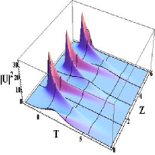
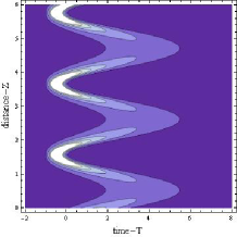
Figure 3: (Color online) (a) The dynamics of chirped bright nonautonomous solitons under periodic dispersion management and $A_{c}=8,\alpha=2,l=3,\omega=3,g=0.25,\beta=1,h=5$ . (b) The contour plot with same parameters. It is obviously that the soliton is ”breathing”,its width and peak oscillate with time, and its center oscillates too.

From these expressions, the soliton is obviously a ”breather” whose shape is changed periodically, shown in Fig.2. Both the width and the peak of nonautonomous soliton are oscillating. This is quite different from the chirp-free nonautonomous soliton under the same dispersion management, which just changes chirp-free nonautonomous soliton’s group velocity, but keeps the shape invariant. This can also be seen by comparing Fig.1 and Fig.2(a). Additionally, to show the character of ”breathing soliton”, we draw the contour plot of Fig.2(a) in Fig.2(b). For $A_{c}\neq 1$, it breathes and its group velocity changes periodically such as Fig.3. Interestingly , chirped nonautonomous soliton with $A_{c}\neq 1$ has characters of both chirp-free one and chirped one with $A_{c}=1$. So, the soliton under periodic dispersion management can evolve as oscillating soliton, or breathing soliton, or oscillating breathing soliton depending on different conditions. This is to be constructive to control the soliton.

If dispersion management is chosen as $l\cos(\omega Z)+l_{0}$, we can also get the evolution of nonautonomous soliton from Eq.(12). When $l_{0}>0$, the soliton will breath more and more lightly with the propagation distance, shown in Fig.4(a); when $l_{0}<0$, it will breath more and more heavily, such as Fig.4(b). This an interesting feature of the soliton in present paper. The above discussions are all made with vanishing gain term. Similarly, one can discuss no vanishing gain term case and find that the gain term does not affect the width and motion of soliton, but changes the peak of soliton. From the Eq.(14), one can find that the soliton’s peak is constant when the gain term becomes $G(Z)=-4\Omega(Z)C_{2}(Z)$.

4 DISCUSSION AND CONCLUSION

In summary, we have deduced the exact bright chirp-free and chirped nonautonomous soliton solutions of the nonlinear equation with arbitrary $Z$-dependent coupling parameters. The functions of such parameters can be seen clearly through the equations describing the evolution of soliton’s center, width and peak. An advantage of present scenario is convenience, one can study the evolution of nonautonomous soliton in various kinds of systems. If the integrability condition is $R=2g\Omega(Z)\exp[\int G(Z)dZ]$, chirp-free soliton can be achieved. The freedom of choosing dispersion management can be used to control the motion of soliton, which does not affect its shape at all with the corresponding nonlinearity. And the gain parameter just affects the peak of the soliton. This provides a lot of particular ways to control the evolution of soliton in waveguide amplifiers or optical fibers. Moreover, for chirp-free solitons without the gain, the classical soliton with unchanged shape can be presented with the condition that the dispersion term $\Omega(Z)$ and nonlinear parameter are related by $R(Z)$ is $R(Z)=2g\Omega(Z)$($g\neq 0$), which is helpful to improve the quality of soliton transmission. For periodic dispersion management $\Omega(Z)=l\cos(\omega Z)$, a novel soliton solution exists, and the center just oscillate and its shape does not change at all.

If the integrability condition $R(Z)=2g\Omega(Z)\exp{[\int G(Z)-4\Omega(Z)C_{2}(Z)dZ]}$ with $C_{2}(Z)=\frac{1}{\int 4\Omega(Z)dZ+h}$ is satisfied, the chirped nonautonomous soliton can be achieved. Especially, the chirped soliton under the same dispersion management $\Omega(Z)=l\cos(\omega Z)$ have been studied. When the gain $G(Z)$ vanishes, there is a novel ”breathing” soliton with the condition $R(Z)=\frac{gl\omega\cos(\omega Z)}{4l\sin(\omega Z)+\omega h}$ and $A_{c}=1$, whose wave center did not oscillate but the shape changed. If $A_{c}\neq 1$, the chirped soliton’ center and its shape will both change under the same dispersion management.

It is worth to point out that the chirp-free nonautonomous soliton in present paper keeps its shape and trajectory unchanged, while the dispersion affect both the trajectory and shape of the chirped nonautonomous soliton. This is quite different form the known dispersion-managed solitons. It provides a possible application in designing some optic apparatus such as amplifier, pulse compressors and etc.

Acknowledgement: This paper was supported by Natural Science Foundation of China granted by No 10975180 and No 10875060.

List of Figure Captions

Fig. 1. (Color online) The dynamics of chirp-free bright temporal nonautonomous soliton under periodic dispersion management for $\alpha=2,l=1,\omega=2,g=0.25,A_{c}=2,\beta=1$.

Fig. 2. (Color online) (a) The dynamics of chirped bright nonautonomous soliton under periodic dispersion management for $\alpha=2;l=3;\omega=3;g=0.25;A_{c}=1;\beta=1;h=5$. (b) The contour plot of (a) with the same parameters. It is obviously that the soliton is ”breathing”, and both width and peak oscillate with time.

Fig. 3. (Color online) (a) The dynamics of chirped bright nonautonomous solitons under periodic dispersion management and $A_{c}=8,\alpha=2,l=3,\omega=3,g=0.25,\beta=1,h=5$ . (b) The contour plot with same parameters. It is obviously that the soliton is ”breathing”,its width and peak oscillate with time, and its center oscillates too.

Fig. 4. (Color online) The dynamics of bright solitons under dispersion management $\Omega(Z)=l\cos(\omega Z)+l_{0}$. (a) $l_{0}=0.03$,the nonautonomous soliton breathes more and more lightly; (b) $l_{0}=-0.03$, it breathes more and more heavily. The other coefficients are: $\alpha=2;l=3;\omega=3;A_{c}=1;g=0.25;\beta=1;h=5$.

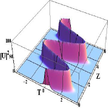
Figure 1: (Color online) The dynamics of chirp-free bright temporal nonautonomous soliton under periodic dispersion management for $\alpha=2,l=1,\omega=2,g=0.25,A_{c}=2,\beta=1$.

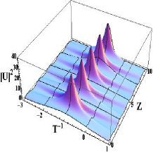
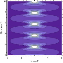
Figure 2: (Color online) (a) The dynamics of chirped bright nonautonomous soliton under periodic dispersion management for $\alpha=2;l=3;\omega=3;g=0.25;A_{c}=1;\beta=1;h=5$. (b) The contour plot of (a) with the same parameters. It is obviously that the soliton is ”breathing”, and both width and peak oscillate with time.

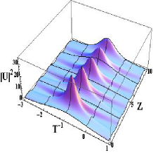
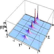
Figure 4: (Color online) The dynamics of bright solitons under dispersion management $\Omega(Z)=l\cos(\omega Z)+l_{0}$. (a) $l_{0}=0.03$,the nonautonomous soliton breathes more and more lightly; (b) $l_{0}=-0.03$, it breathes more and more heavily. The other coefficients are: $\alpha=2;l=3;\omega=3;A_{c}=1;g=0.25;\beta=1;h=5$.

References

- [1] A. Hasegawa, F. Tappert, “Transmission of stationary nonlinear optical pulses in dispersive dielectric fibers. I. Anomalous dispersion,” Appl. Phys. Lett. 23, 142-144 (1973).
- [2] A. Hasegawa, F. Tappert, “Transmission of stationary nonlinear optical pulses in dispersive dielectric fibers. II. Normal dispersion,” Appl. Phys. Lett. 23, 171-172 (1973).
- [3] L. F. Mollenauer, R. H. Stolen, and J. P. Gordon, “Experimental Observation Of Picosecond Pulse Narrowing And Solitons In Optical Fibers,” Phys. Rev. Lett. 45, 1095-1098 (1980).
- [4] H. G. Luo, D. Zhao, and X. G. He, “Exactly controllable transmission of nonautonomous optical soliton,” Phys. Rev. A 79, 063802 (2009).
- [5] L. F. Mollenauer and K. Simth, “Demonstration of soliton transmission over more than 4000 kmin fiber with loss periodically compensated by Raman gain,” Optics. Letters. 13, 675 - 677 (1988).
- [6] M. Nakazawa, H. Kubota, K. Suzuki, E. Yamada and A. Sahara, “Recent progress in soliton transmission technology,” Chaos 10, 486 - 514 (2000).
- [7] M. Senturion, M. A. Porter, P. G. Kevrekidis and D.Psaltis, “Nonlinearity managament in optics: experiment, thoery, and simulation,” Phys. Rev. Lett. 97, 033903 (2006).
- [8] V. N. Serkin and A. Hasegawa, “Novel solition solution of the nonlinear Schrödinger equation model,” Phys. Rev. Lett. 85, 4502-4505 (2000).
- [9] V. N. Serkin and A. Hasegawa, and T. L. Belyaeva, “Nonautonomous solitons in external potentials,” Phys. Rev. Lett. 98, 074102 (2007),
- [10] V. N. Serkin, A. Hasegawa, and T.L. Belyaeva, “Nonautonomous matter wave solitons near Feshbach resonance,” Phys. Rev. A 81, 023610 (2010).
- [11] V. I. Kruglov, A. C. Peacock, and J. D. Harvey, “Exact Self-Similar Solutions of the Generalized Nonlinear Schrödinger Equation with Distributed Coefficients,” Phys. Rev. Lett. 90, 113902 (2003).
- [12] S. A. Ponomarenko and G. P. Agrawal, “Interactions of chirped and chirp-free similaritons in optical fiber amplifiers,” Opt. Express 15, 2963 - 2973 (2007).
- [13] V. I. Kruglov, A. C. Peacock, J. M. Dudley, J. D. Harvey, “Self-similar propagation of higher-power parabolic pulse in optical fiber amplifiers,” Opt. Lett. 25, 1753 - 1755 (2000).
- [14] B. A. Malomed, “Soliton Management in Periodic Systems,” Springer, New York (2006).
- [15] D. J. Richardson, R. P. Chamberlin, L. Dong, and D. N. Payne, “High quality soliton loss-compensation in 38 km dispersion-decreasing fibre,” Electron. Lett. 31, 1681 - 1682 (1995).
- [16] A. J. Stentz, R. Boyd and A. F. Evans, “Dramatically improved transmission of ultrashort solitons through 40 km of dispersion-decreasing fiber,” Opt. Lett. 20, 1770 - 1772 (1995).
- [17] D. J. Richardson, L. Dong, R. P. Chamberlin, A. D. Ellis, T. Widdowson and W. A. Pender, “Periodically amplified system based on loss compensating dispersion decreasing fibre,” Electron. Lett. 32, 373 (1996).
- [18] K. Suzuki, H. Kubota, A. Sahara, and M. Nakazawa, “640 Gbit/s (40 Gbit/s 16 channel) dispersion-managed DWDM soliton transmission over 1000 km with spectral efficiency of 0.4 bit/Hz,” Electron. Lett. 36, 443 - 445 (2000).
- [19] M. Nakazawa, H. Kubota, K. Suzuki, E. Yamada, and A. Sahata, “Ultrahigh-speed long-distance TDM and WDM soliton transmission technologies,” IEEE J. Sel. Top. Quantum Electron. 6, 363 - 396 (2000).
- [20] L. F. Mollenauer, P. V. Mamyshev, J. Gripp, M. J. Neubelt, N. Mamysheva, L. Gruner-Nielsen, and T. Veng, “Demonstration of massive wavelength-division multiplexing over transoceanic distances by use of dispersion-managed solitons,” Opt. Lett. 25, 704 - 706 (2000).
- [21] G. P. Agrawal, “Nonliear Fiber Optics,” Third Edition (Academic Press, 2001).