Effect of edge decoration on the energy spectrum of semi-infinite lattices

Abstract

Analytical studies of the effect of edge decoration on the energy spectrum of semi-infinite one-dimensional (1D) lattice chain with Peierls phase transition and zigzag edged graphene (ZEG) are presented by means of transfer matrix method, in the frame of which the sufficient and necessary conditions for the existence of the edge states are determined. For 1D lattice chain, the zero-energy edge state exists when Peierls phase transition happens regardless whether the decoration exists or not, while the non-zero-energy edge states can be induced and manipulated through adjusting the edge decoration. On the other hand, the semi-infinite ZEG model with nearest-neighbor interaction can be mapped into the 1D lattice chain case. The non-zero-energy edge states can be induced by the decoration as well, and we can obtain the condition of the decoration on the edge for the existence of the novel edge states.

I Introduction

One of the interesting phenomena in condensed matter physics is the existence of edge states, the properties of which are distinct from those of the bulk states. There are some examples showing that the system is insulated in the bulk, while conduction can be allowed by edge states on the boundary. The most prominent ones are the quantum Hall effect (QHE)QHE ; LaughlinQHE ; HalperinQHE ; Bhatt and the quantum spin Hall effect (QSHE)Kane1 ; Bernevig1 ; Bernevig2 , where the quantization of a Hall conductance is tightly associated with the edge statesLaughlinQHE ; HalperinQHE ; Bhatt ; Kane1 ; Bernevig1 ; Bernevig2 ; Thouless ; Kohmoto ; Hatsugai1 ; Qi1 ; Kane2 ; Kane3 .

With the development of grapheneNovoselov1 ; Novoselov2 in recent years, the edge states of graphene modelCastro attract much attention. From the topological view, edge states can be induced in the system with different structures of edgesKlein ; Fujita ; in experiments, with the help of scanning tunneling microscopy and scanning tunneling spectroscopy, the presence of structure-dependent edge states of graphite can be observedNiimi ; Kobayashi . As we know, some results of the edge states have been reported in the tight-binding modelFujita ; Nakada ; Wakabayashi ; Kusakabe ; Peres ; Ezawa ; Hasegawa1 ; Hasegawa2 , Dirac equationBrey ; Sasaki ; Abanin , the transfer matrix method (TMM) calculationDHLee ; LJiang ; Haidong ; Li-Tao , first principles calculationsMiyamoto ; Okada ; Lee , and most of them focus on the zero mode of the graphene nanoribbon, while some consider about the effects of disorder or the edge corrections.

In this paper, we report a systematic study of the zero-energy and non-zero-energy edge states caused by the decoration on the edge by means of TMM. We analytically study the simple tight-binding model of semi-infinite 1D lattice chain and the zigzag edged graphene (ZEG), and the consequent novel edge states that arise due to the edge decoration, which is the hopping interaction on the edge being different from that in the bulk, caused as edge binding softening or stiffening. The extended states and the localized edge states are also discussed, and the analytical relations of the edge states with the edge decoration can be obtained as well. It might be applicable in future devices since novel edge states, particularly in the energy forbidden region, could significantly change the optical property, even the transportation.

The rest of this paper is organized as follows. In Sec. II, we take a semi-infinite 1D Peierls chain model as a fundamental case to show the relation of edge states with phase transition and describe how the analytical relations can be obtained efficiently through TMM for not only the extended states, but also the edge states. The sufficient and necessary conditions (SNC) for the existence of the edge states are determined. With the general discussion of the 1D chain model, in Sec. III, we map it to the ZEG, with applying the rigorous results in Sec. II to obtain the edge states of ZEG with and without edge decoration. Finally, we give a brief conclusion in Sec. IV.

II EDGE STATES AND PEIERLS PHASE TRANSITION

As a typical example for studying edge states occurring in semi-infinite systems due to phase transition, we treat a semi-infinite 1D lattice chain that can occur Peierls phase transition. It has been well-known that 1D periodic atomic chain is not stable due to the electron-phonon interaction that drives chain to have pairing transition. In the case of half-filling electrons, the atoms in a periodic lattice chain like to pair together, forming Peierls pairing state. Its geometrical structure is shown in Fig. 1, where one unit cell includes two atoms. In the tight-binding approximation, consider just the nearest-neighbor interaction (n.n.), two different n.n. hopping constants are $t_{1}(=t\pm\Delta)$ and $t_{2}(=t\mp\Delta)$ separately, where $t$ is the hopping constant before Peierls phase transition, $\Delta(\geqslant 0)$ describes the pairing phase transition just like the phase transition in 1D molecule polyacetylene. $\Delta=0$ when Peierls phase transition is suspended. In general, $t_{1}\neq t_{2}$ if $\Delta\neq 0.$ The chain with Peierls pairing is equivalent to a 1D model of atomic chain in which each cell has two atoms, which are denoted in a cell as $A$ and $B$. The edge of the semi-infinite chain is set at the left terminal. Without loss of generality, we assume that the lattice at left terminal is $A$ denoted as $1$, and label the unit cell with an integer number ordered from the left terminal to the right infinity. Since a non-Bravais lattice with two atoms per unit cell is bipartite, we have defined two kinds of fermion operators, $\varphi_{iA}$ and $\varphi_{iB}$, where $i$ is the integer index labeling the unit cell. The Hamiltonian can be approximated by

$$H=t_{0}\varphi_{1A}^{{\dagger}}\varphi_{1B}+t_{1}\sum_{i\geqslant 1}\varphi_{i+1A}^{{\dagger}}\varphi_{iB}+t_{2}\sum_{i\geqslant 2}\varphi_{iA}^{{\dagger}}\varphi_{iB}+h.c.$$ (1)

where $t_{0},t_{1},t_{2}$ are three hopping parameters, and set all of them to be positive. The parameter $t_{0}$ is introduced to describe edge decoration. From Eq. (1), we can derive the dynamical equationsHarper through defining an elemental excitation with energy $E$ as follows

$$\begin{cases}E\varphi_{1A}&=\quad t_{0}\varphi_{1B}\\ E\varphi_{1B}&=\quad t_{0}\varphi_{1A}+t_{1}\varphi_{2A}\\ E\varphi_{iA}&=\quad t_{2}\varphi_{iB}+t_{1}\varphi_{i-1B}\quad(i\geqslant 2)\\ E\varphi_{iB}&=\quad t_{2}\varphi_{iA}+t_{1}\varphi_{i+1A}\quad(i\geqslant 2)\end{cases}$$ (2)

According to above equations, we try to get the bulk wave-functions, and find out the physically meaningful localized states which decay from the surface. When $E=0$ or $E\neq 0$, the above equations will be in different forms, so in the following subsection, we will discuss them separately.

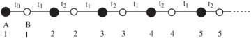
Figure 1: Schematic illustration of the lattice structure of 1D semi-infinite chain with the closed (black) circles and the open (white) circles, consisting of sublattices $A$ and $B$.

Under the condition $E=0$, Eq. (2) can be reduced to the decoupled ones:

$$\begin{cases}\qquad\qquad t_{0}\varphi_{1B}&=\quad 0\\ t_{0}\varphi_{1A}+t_{1}\varphi_{2A}&=\quad 0\\ t_{2}\varphi_{iB}+t_{1}\varphi_{i-1B}&=\quad 0\quad(i\geqslant 2)\\ t_{2}\varphi_{iA}+t_{1}\varphi_{i+1A}&=\quad 0\quad(i\geqslant 2)\end{cases}$$ (3)

From Eq. (3), it is easy to know that the wave-functions of all the type $B$ sublattices will be equal to zero: $\{\varphi_{iB}=0:i=1,2,\cdots,\infty\}$; meanwhile the wave-function of sublattice $A$ in the $n$ unit cell will be:

$$\varphi_{nA}=\left(-\frac{t_{2}}{t_{1}}\right)^{n-2}\left(-\frac{t_{0}}{t_{1}}\right)\varphi_{1A},\qquad n=2,3,4\cdots$$ (4)

$\varphi_{1A}$ is the initial value of wave excitation with zero energy at edge site. $t_{2}=t_{1}$ corresponds to the extended state in bulk. If $t_{1}\neq t_{2}$, in order to obtain the physically meaningful edge states, we must restrict $t_{2}/t_{1}<1$, so that when $n$ goes to infinity, the wave-functions of sublattice $A$ will approach to $0$, showing the state is localized near the edge region. Away from the surface, the amplitude of the wave-function will exponentially decay as $e^{-n2a/\lambda_{L}}$. The localized length $\lambda_{L}$ of the edge state is $2a/(\ln t_{2}-\ln t_{1})$, where $2a$ is the periodic constant of the cell after Peierls pairing. Thus, we can conclude that zero-energy edge state can exist due to Peierls phase transition when $t_{2}<t_{1}$ $(\Delta\neq 0)$, and this result can be obtained by surface Green’s functionPeres1 . It is shown that no matter whether the edge decoration exists or not, zero-energy edge state is not affected by edge decoration $t_{0}(\neq t_{2})$. 1D Peierls pairing mode is an example to demonstrate that the studies of zero-energy edge state could show some evidence of the phase transition, even the mechanism of phase transition.

In the following, we will study whether the non-zero-energy edge states can exist or not. According to Eq. (2), after eliminate sublattice $A$ and $B$ separately, we can obtain

$$\begin{cases}E^{2}\varphi_{1A}=t_{0}^{2}\varphi_{1A}+t_{0}t_{1}\varphi_{2A}\\ E^{2}\varphi_{2A}=(t_{1}^{2}+t_{2}^{2})\varphi_{2A}+t_{0}t_{1}\varphi_{1A}+t_{1}t_{2}\varphi_{3A}\\ E^{2}\varphi_{iA}=(t_{1}^{2}+t_{2}^{2})\varphi_{iA}+t_{1}t_{2}\varphi_{i-1A}+t_{1}t_{2}\varphi_{i+1A},i\geqslant 3,\end{cases}$$ (5)

and

$$\begin{cases}E^{2}\varphi_{1B}=(t_{0}^{2}+t_{1}^{2})\varphi_{1B}+t_{1}t_{2}\varphi_{2B},\\ E^{2}\varphi_{iB}=(t_{1}^{2}+t_{2}^{2})\varphi_{iB}+t_{1}t_{2}\varphi_{i-1B}+t_{1}t_{2}\varphi_{i+1B},i\geqslant 2\end{cases}$$ (6)

According to the first equation in Eq. (5), we introduce a fictitious $\varphi_{0A}=0$ into our discussion without lose of generality. Then we can turn Eq. (5) into matrix forms:

$$\left(\begin{array}[]{c}\varphi_{i+1A}\\ \varphi_{iA}\end{array}\right) = T^{i-2}\left(\begin{array}[]{c}\varphi_{3A}\\ \varphi_{2A}\end{array}\right)\quad(i\geqslant 3)$$ (11)

$$\left(\begin{array}[]{c}\varphi_{3A}\\ \varphi_{2A}\end{array}\right) = T_{1}\left(\begin{array}[]{c}\varphi_{2A}\\ \varphi_{1A}\end{array}\right)$$ (16)

$$\left(\begin{array}[]{c}\varphi_{2A}\\ \varphi_{1A}\end{array}\right) = T_{2}\left(\begin{array}[]{c}\varphi_{1A}\\ \varphi_{0A}\end{array}\right)$$ (21)

where $T$, $T_{1}$ and $T_{2}$ are defined as

$$T = \left(\begin{array}[]{cc}\alpha&-1\\ 1&0\end{array}\right)$$ (24)

$$T_{1} = \left(\begin{array}[]{cc}\alpha&-\frac{t_{0}}{t_{2}}\\ 1&0\end{array}\right)$$ (27)

$$T_{2} = \left(\begin{array}[]{cc}\beta&-1\\ 1&0\end{array}\right)$$ (30)

with $\alpha=(E^{2}-t_{1}^{2}-t_{2}^{2})/t_{1}t_{2}$ and $\beta=(E^{2}-t_{0}^{2})/t_{0}t_{1}.$ Meanwhile, the wave-functions of the sublattices $B$ satisfy the relations:

$$\left(\begin{array}[]{c}\varphi_{i+1B}\\ \varphi_{iB}\end{array}\right) = T^{i-1}\left(\begin{array}[]{c}\varphi_{2B}\\ \varphi_{1B}\end{array}\right)\quad,(i\geqslant 2);$$ (35)

$$\varphi_{2B} = \gamma\varphi_{1B};\varphi_{1B}=\frac{E}{t_{0}}\varphi_{1A}$$ (36)

and $\gamma=(E^{2}-t_{0}^{2}-t_{1}^{2})/t_{1}t_{2}$. The energy $E$ must be real for the physical quantity, and all $\alpha,\beta$ and $\gamma$ are real numbers. Diagonalize the transfer matrix $T$ to $D=U^{-1}TU$, and we have

$$\begin{cases}\left(\begin{array}[]{c}\varphi_{i+1A}\\ \varphi_{iA}\end{array}\right)=UD^{i-2}U^{-1}T_{1}T_{2}\left(\begin{array}[]{c}\varphi_{1A}\\ \varphi_{0A}\end{array}\right)\\ \left(\begin{array}[]{c}\varphi_{i+1B}\\ \varphi_{iB}\end{array}\right)=UD^{i-1}U^{-1}\left(\begin{array}[]{c}\gamma\\ 1\end{array}\right)\frac{E}{t_{0}}\varphi_{1A}.\end{cases}$$ (37)

with

$$D=\left(\begin{array}[]{cc}\lambda_{-}&0\\ 0&\lambda_{+}\end{array}\right)\qquad U=\left(\begin{array}[]{cc}\lambda_{-}&\lambda_{+}\\ 1&1\end{array}\right)$$ (38)

$$U^{-1}=\frac{1}{\sqrt{\alpha^{2}-4}}\left(\begin{array}[]{cc}-1&\lambda_{+}\\ 1&-\lambda_{-}\end{array}\right)$$ (39)

where $\lambda_{-}=\frac{1}{2}(\alpha-\sqrt{\alpha^{2}-4})$ and $\lambda_{+}=\frac{1}{2}(\alpha+\sqrt{\alpha^{2}-4})$. Eq. (37) can be rewritten as

$$\begin{cases}\left(\begin{array}[]{c}\varphi_{n+3A}\\ \varphi_{n+2A}\end{array}\right)=U\left(\begin{array}[]{c}\Gamma_{1}\lambda_{-}^{n}\\ \Gamma_{2}\lambda_{+}^{n}\end{array}\right)\varphi_{1A},\\ \left(\begin{array}[]{c}\varphi_{n+3B}\\ \varphi_{n+2B}\end{array}\right)=U\left(\begin{array}[]{c}\Theta_{1}\lambda_{-}^{n}\\ \Theta_{2}\lambda_{+}^{n}\end{array}\right)\dfrac{E}{t_{0}}\varphi_{1A}.\end{cases}$$ (40)

Where $\Gamma_{1}=U_{11}^{-1}\left(\alpha\beta-\frac{t_{0}}{t_{2}}\right)+U_{12}^{-1}\beta$, $\Gamma_{2}=U_{21}^{-1}\left(\alpha\beta-\frac{t_{0}}{t_{2}}\right)+U_{22}^{-1}\beta$, $\Theta_{1}=U_{11}^{-1}\gamma+U_{12}^{-1}$, $\Theta_{2}=U_{21}^{-1}\gamma+U_{22}^{-1}$. We must request $\varphi_{1A}\neq 0,$ otherwise the wave function vanishes $\{\varphi_{iA}=\varphi_{iB}=0:i=1,2,\cdot\cdot\cdot,\infty\}$.

When $|\alpha|\leqslant 2$, $|\lambda_{-}|=|\lambda_{+}|=1$. It corresponds to the extended states in the bulk. Thus, all energy $E^{2}$ satisfying the energy inequality $|E^{2}-t^{2}_{1}-t^{2}_{2}|/|t_{1}t_{2}|\leqslant 2$ must associate with the extended states. With the Eq. (5) and Eq. (6), considering a continuous parameter $k_{x}$ to keep $|\cos(k_{x}a)|\leqslant 1$, we can get the dispersion relation of the bulk states as:

$$E^{2}=t_{1}^{2}+t_{2}^{2}+2t_{1}t_{2}\cos(k_{x}a),~{}k_{x}a\in[-\pi,\pi].$$ (41)

In the case, we have $\lambda_{\pm}=e^{\pm ik_{x}a}$. From Eq. (40), the $k_{x}$ belonging to $\mathbb{R}$ is clearly served as a wave vector of this extended mode propagating along the chain direction. The left edge makes the semi-infinite chain to have two waves interfered. One is the $e^{ik_{x}na}$, the other is $e^{-ik_{x}na}$.

In the following, we focus on the solution of edge state when the condition $|\alpha|>2$ is satisfied. In the case of $\alpha>2$, we get $0<\lambda_{-}<1$ and $\lambda_{+}>1$, while $\lambda_{-}<-1$ and $-1<\lambda_{+}<0$ for the case of $\alpha<-2$. We will discuss these two cases respectively.

In the case of $\alpha>2$, it yields $0<\lambda_{-}<1$, $\lambda_{+}>1$. The necessary conditions to have a stable edge states localized at edge boundary must be $\Gamma_{2}=0$ and $\Theta_{2}=0$ that are

$$U_{21}^{-1}\left(\alpha\beta-\frac{t_{0}}{t_{2}}\right)+U_{22}^{-1}\beta = 0$$

$$U_{21}^{-1}\gamma+U_{22}^{-1} = 0$$

From Eq. (38), Eq. (39) and the definitions of $\lambda_{\pm}$, above two equations can be changed to the following:

$$\begin{cases}(\alpha+\sqrt{\alpha^{2}-4})\beta-2\dfrac{t_{0}}{t_{2}}=0,\\ \sqrt{\alpha^{2}-4}-\alpha+2\gamma=0\end{cases}$$ (42)

where $\alpha,\beta$ and $\gamma$ are the functions of energy $E(\neq 0)$. Eq. (42) is the necessary condition for the occurrence of non-zero-energy edge state. If Eq. (42) can not be satisfied for any finite energy $E$, the non-zero-energy edge states could not exist. Inputting the definitions of $\alpha,\beta$ and $\gamma$ into Eq. (42), we obtain

$$(t_{0}^{2}-t_{2}^{2})(E^{2}-t_{0}^{2})=t_{0}^{2}t_{1}^{2}$$

When the edge has no decoration, $t_{0}=t_{2}(\neq 0)$, there should be no finite solution of $E$ for above equation since $t_{0}^{2}t_{1}^{2}\neq 0$. Thus we conclude that non-zero-energy edge state does not exist in 1D Peierls chain without edge decoration. When $t_{0}\neq t_{2}$, we have solution

$$E^{2}=t_{0}^{2}+t_{0}^{2}t_{1}^{2}/\left(t_{0}^{2}-t_{2}^{2}\right).$$ (43)

Due to $\alpha>2$, we obtain $E^{2}>(t_{1}+t_{2})^{2}>0$, which corresponds to a stable edge state. With the definition of $\gamma$ and $\alpha$, we get $\gamma=\alpha-\left(t_{0}^{2}-t_{2}^{2}\right)/t_{1}t_{2}$. Taking it back to Eq. (42), we have

$$\left(t_{0}^{2}-t_{2}^{2}\right)/t_{1}t_{2}=\frac{\alpha}{2}+\frac{\sqrt{\alpha^{2}-4}}{2}>1$$

Thus the condition to get an additional stable non-zero-energy edge state is the inequality $t_{0}^{2}>t_{2}^{2}+t_{1}t_{2}$. An appropriate manipulation on the edge decoration $t_{0}$ can induce the non-zero-energy edge state. There is no constraint showing the quantity relation between $t_{1}$ and $t_{2}$. From previous subsection, it has been known that the zero-energy edge state can exist with $t_{2}/t_{1}<1$, so the zero mode and the non-zero-energy edge states can appear at the same time. However, there will be non-zero-energy edge states only if $t_{2}\geqslant t_{1}$ together with $t_{0}^{2}>t_{2}^{2}+t_{1}t_{2}$.

Similarly we can get constraints for $\alpha<-2$

$$(\alpha-\sqrt{\alpha^{2}-4})\beta-2\frac{t_{0}}{t_{2}} = 0$$

$$\sqrt{\alpha^{2}-4}+\alpha-2\gamma = 0$$

They also yield the same energy condition: $E^{2}=t_{0}^{2}+t_{0}^{2}t_{1}^{2}/\left(t_{0}^{2}-t_{2}^{2}\right)$. And besides $\gamma=\alpha-\left(t_{0}^{2}-t_{2}^{2}\right)/t_{1}t_{2}$, when $\alpha<-2$, it is easy to get:

$$\left(t_{0}^{2}-t_{2}^{2}\right)/t_{1}t_{2}=\frac{\alpha}{2}-\frac{\sqrt{\alpha^{2}-4}}{2}<-1$$

We can find that the non-zero-energy edge state can also exist under the condition: $t_{0}^{2}<t_{2}(t_{2}-t_{1})$ that requests $t_{2}>t_{1}$ and results zero-energy edge state vanishing.

From above two cases, we can see that non-zero-energy edge states are tightly related with edge decoration $t_{0}$ and can be manipulated by decorating the edge atoms.

We conclude that a zero-energy edge state will appear if Peierls transition happens $(t_{2}<t_{1})$ regardless edge decoration at all. A non-zero-energy edge state can occur due to some edge decoration as following condition:

$$\begin{cases}E^{2}=t_{0}^{2}+t_{0}^{2}t_{1}^{2}/\left(t_{0}^{2}-t_{2}^{2}\right)(>0,t_{0}\neq t_{2}):\\ t_{0}^{2}>t_{2}^{2}+t_{1}t_{2}>0;~{}\text{or}~{}t_{0}^{2}<t_{2}(t_{2}-t_{1}),~{}t_{2}>t_{1}.\end{cases}$$ (44)

Non-zero-energy edge state can be manipulated with decorating the edge.

III EDGE STATES OF SEMI-INFINITE ZEG

In this section, we would present some analytical results for the edge states of ZEG. Although some results has been reportedLJiang for uniform ZEG ribbon, and can be extended to semi-infinite ZEG through size scaling to the infinite width of ribbon, the effect of edge decoration on the edge states has not been reported. Thus we will supply some analytical results on the occurrence of non-zero-energy edge states and its energy dispersion in semi-infinite ZEG with edge decoration. In the previous section, we have obtained some criteria on the existence of edge states in semi-infinite 1D Peierls model with and without edge decoration. In fact, some 2D and 3D lattice models could be reduced into above 1D model such as the model of ZEG to be discussed in this section. The geometrical structure of graphene is shown in Fig. 2. Without loss of generality, we denote the the first left line $1_{A}$ as an edge, and take the lattice system in $y$ direction to be infinite and periodic with constant $a$. Then the semi-infinite ZEG can be described by a line set with infinite number of periodic 1D perpendicular chain along $y$ direction: $\{1_{A},1_{B},...,n_{A},n_{B},\cdots\}.$ The positions of sublattices $A$ and $B$ are labeled by two indices $\{i,y_{i,A(B)}\}$ where $i$ labels the number of perpendicular line from $1$ to $\infty$. After Fourier transformation for $\{y_{i,A(B)}\}$ with periodic constant $a,$ in second quantization representation, the model Hamiltonian with n.n. hopping can be expressed by a set of the Fermion operators $\{\phi_{i,A(B)}(k_{y}):i=1,2,...,\infty\}$:

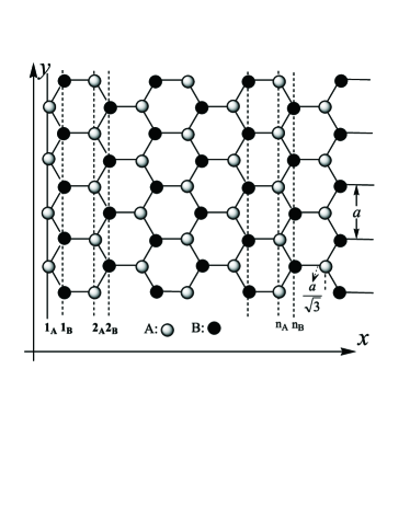
Figure 2: Schematic illustration of the lattice structure of semi-infinite zigzag edged graphene, the fulfilled circles represent the sublattice $B$, others are the sublattice $A$. The left first line $1_{A}$ is the zigzag edge of the graphene.

$$H = \sum_{k_{y},i\geqslant 2}t\phi_{i,A}^{{\dagger}}\left(k_{y}\right)\phi_{i-1,B}(k_{y})+\tilde{t}\phi_{i,A}^{{\dagger}}\left(k_{y}\right)\phi_{i,B}\left(k_{y}\right)$$ (45)

$$+ \sum_{k_{y}}\tilde{t}_{0}\phi_{1,A}^{{\dagger}}(k_{y})\phi_{1,B}(k_{y})+h.c.,$$

where $k_{y}$ is a good quantum number, $\tilde{t}=2t\cos(k_{y}a/2)$ and $\tilde{t}_{0}=2t^{\prime}_{0}\cos(k_{y}a/2)$. We have introduced a simplified edge hopping decoration $t^{\prime}_{0}$ at first line. When $t^{\prime}_{0}=t,$ it becomes an ideal semi-infinite ZEG without edge decoration. In general, $t^{\prime}_{0}\neq t$ that describes some edge decoration, and we set all the hopping interaction positive as well. The wave function at site $(i,j)$ of $A(B)$ sublattice is written as $\Psi_{A(B)}^{(i,j)}(k_{y})=\exp(ik_{y}y_{j,A(B)})\phi_{i,A(B)}(k_{y})$.

For each fixed $k_{y}$, the Hamiltonian of Eq. (45) is equivalent to the 1D Peierls chain in Sec. II when we denote $t_{0}=\tilde{t}_{0}$, $t_{1}=t$ and $t_{2}=\tilde{t}$. Thus the conclusion in Sec. II can be applied to study the ZEG.

Comparing with standard energy spectrum of bulk graphene, $\alpha=\frac{E^{2}-4t^{2}\cos^{2}{k_{y}a/2}-t^{2}}{2t^{2}\cos{k_{y}a/2}}$, when $\alpha^{2}\leqslant 4$, we can get the dispersion relation for extended states:

$$E^{2} = t^{2}_{1}+t^{2}_{2}+2t_{1}t_{2}\cos(\sqrt{3}k_{x}a/2)$$

$$= t^{2}[1+4\cos^{2}(k_{y}a/2)+4\cos(k_{y}a/2)\cos(\sqrt{3}k_{x}a/2)]$$

This is the standard formula of the energy spectrum of the infinite bulk graphene.

In the following, we would focus on the edge states. From Sec. II, the necessary condition for the existence of zero-energy edge state is $|t_{2}/t_{1}|<1$ that directly results the condition $|2\cos(k_{y}a/2)|<1$ for ZEG. It clearly shows the well-known conclusion that a zero-energy edge state exists in the region $k_{y}a\in(2\pi/3,4\pi/3)$ for ZEG. But the point of $k_{y}a=\pm\pi$ must be excluded since $t_{2}=2t\cos(k_{y}a/2)=2t\cos(\pi/2)=0$ that corresponds to an internal mode within the isolated chains. From the conclusion of 1D model in Sec.II, we also can conclude that the zero-energy edge state is stable.

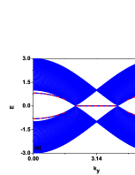
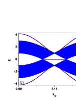
Figure 3: (color online) By exact diagonalization method, the dispersion relation of the bulk states and the edge state are depicted (blue line), while the dispersion relation of the edge state obtained through TMM is depicted in the dashed line (red dash-line). Parameters: (a) $t^{\prime}_{0}=0.5t$, (b) $t^{\prime}_{0}=2.0t$.

Just as the discussion shown in the above section, the SNC for the existence of the non-zero-energy edge states should be discussed with $\alpha^{2}>4$. With similar discussions, we can get the dispersion of energy spectrum of non-zero-energy edge states as follows:

$$E^{2}=4t^{\prime 2}_{0}\cos^{2}{(k_{y}a/2)}+\frac{t^{\prime 2}_{0}t^{2}}{t^{\prime 2}_{0}-t^{2}}$$ (47)

while the SNC for the existence of those states must satisfy:

$$\begin{cases}t^{\prime}_{0}<t,\;0<\frac{t^{2}}{2(t^{2}-t^{\prime 2}_{0})}<|\cos{(k_{y}a/2)}|\leqslant 1\\ \qquad\qquad\Longrightarrow t^{2}>2t^{\prime 2}_{0};\\ \text{or}\\ t^{\prime}_{0}>t,\;0<\frac{t^{2}}{2(t^{\prime 2}_{0}-t^{2})}<|\cos{(k_{y}a/2)}|\leqslant 1\\ \qquad\qquad\Longrightarrow t^{2}<2t^{\prime 2}_{0}/3\end{cases}$$ (48)

As above shown, we can easily see that the existence of the non-zero-energy edge states depends on the decoration on the edge, the ratio between the edge hopping and the bulk hopping should be within a certain threshold, so that we can detect the finite-energy edge states. Comparing the results obtained above with those by the means of the exact diagonal method on a finite-size zigzag nanoribbon model, the results are accordance with each other, as shown in Fig. 3.

IV Conclusions

We have studied the semi-infinite 1D lattice chain with Peierls phase transition and ZEG model respectively, with the help of TMM. We focus on the zero-energy edge states and non-zero-energy edge states, under the condition of the edge decoration, which is the electron hopping energy being different from that in bulk. In the 1D model, we conclude that a zero-energy edge state will appear if Peierls transition happens regardless edge decoration at all. A non-zero-energy edge state can occur due to the edge decoration. Then we map the 1D case into the ZEG. Suppose the electron hopping energy is $t^{\prime}_{0}$, different from that $t$ in bulk because of the boundary effects. It is found that the existence of the zero-energy edge states is independent of the magnitude of $t^{\prime}_{0}$. In addition to the zero-energy edge states, there can exist edge states of finite energy if $t>\sqrt{2}t^{\prime}_{0}$ or $t<\sqrt{2/3}t^{\prime}_{0}$. These edge states appear as pairs with energy $\pm E$ outside of the continuum conduction and valence bands.

- (1) The Quantum Hall Effect, 2nd Ed., edited by R. E. Prange and S. M. Girvin (Springer-Verlag, New York, 1990).
- (2) R. B. Laughlin, Phys. Rev. B 23, 5632 (1981).
- (3) B. I. Halperin, Phys. Rev. B 25, 2185 (1982).
- (4) D. P. Arovas, R. N. Bhatt, F. D. M. Haldane, P. B. Littlewood, and R. Rammal, Phys. Rev. Lett. 60, 619 (1988).
- (5) C. L. Kane and E. J. Mele, Phys. Rev. Lett. 95, 226801 (2005).
- (6) B.A. Bernevig and S. C. Zhang, Phys. Rev. Lett. 96, 106802 (2006).
- (7) B. A. Bernevig, T. L. Hughes, and S. C. Zhang, Science 314, 1757 (2006).
- (8) D. J. Thouless, M. Kohmoto, M. P. Nightingale, and M. den Nijs, Phys. Rev. Lett. 49, 405 (1982).
- (9) M. Kohmoto, Ann. Phys. (N.Y.) 160, 355 (1985).
- (10) Y. Hatsugai, Phys. Rev. Lett. 71 3697 (1993).
- (11) X. L. Qi, Y. S. Wu, and S. C. Zhang, Phys. Rev. B 74, 045125 (2006).
- (12) L. Fu and C. L. Kane, Phys. Rev. B 74, 195312 (2006).
- (13) C. L. Kane and E. J. Mele, Phys. Rev. Lett. 95, 146802 (2005).
- (14) K. S. Novoselov, A. K. Geim, S. V. Morozov, D. Jiang, Y. Zhang, S. V. Dubonos, I. V. Grigorieva, and A. A. Firsov, Science 306, 666 (2004).
- (15) K. S. Novoselov, A. K. Geim, S. V. Morozov, D. Jiang, M. I. Katsnelson, I. V. Grigorieva, S. V. Dubonos, and A. A. Firsov, Nature 438, 197 (2005).
- (16) Y. Niimi, T. Matsui, H. Kambara, K. Tagami, M. Tsukada, and H. Fukuyama, Appl. Surf. Sci. 241, 43 (2005).
- (17) Y. Kobayashi, K. I. Fukui, T. Enoki, K. Kusakabe, and Y. Kaburagi, Phys. Rev. B 71, 193406 (2005).
- (18) A. H. Castro Neto et al., Rev. Mod. Phys. 81, 109 (2009).
- (19) D. J. Klein, Chem. Phys. Lett 217, 261 (1994).
- (20) K. Nakada, M. Fujita, G.Dresselhaus, and M. S. Dresselhaus, Phys. Rev. B 54, 17954 (1996).
- (21) K. Nakada, M. Fujita, G. Dresselhaus, and M. S. Dresselhaus, Phys. Rev. B 54, 17954 (1996).
- (22) K. Wakabayashi, M. Fujita, H. Ajiki, and M. Sigrist, Phys. Rev. B 59, 8271 (1999).
- (23) K. Kusakabe and Y. Takagi, Mol. Cryst. Liq. Cryst. Sci. Technol.,Sect. A 387, 7 (2002).
- (24) M. Ezawa, Phys. Rev. B 73, 045432 (2006).
- (25) N. M. R. Peres, F. Guinea, and A. H. Castro Neto, Phys. Rev. B 73, 125411 (2006).
- (26) Y. Hasegawa, R. Konno, H. Nakano, and M. Kohmoto Phys. Rev. B 74, 033413 (2006).
- (27) M. Kohmoto and Y. Hasegawa, Phys. Rev. B 76, 205402 (2007).
- (28) L. Brey and H. A. Fertig, Phys. Rev. B 73, 235411 (2006).
- (29) K. Sasaki, S. Murakami, and R. Saito, J. Phys. Soc. Jpn. 75, 074713 (2006).
- (30) D. A. Abanin, P. A. Lee, and L. S. Levitov, Phys. Rev. Lett. 96, 176803 (2006).
- (31) D. H. Lee and J.D. Joannopoulos, Phys. Rev. B 23, 4988 (1981), Phys. Rev. B 24, 6899 (1981).
- (32) Liwei Jiang, Yisong Zheng, Cuishan Yi, Haidong Li, and Tianquan Lu, Phys. Rev. B 80, 155454 (2009).
- (33) Haidong Li, Lin Wang, Zhihuan Lan, and Yisong Zheng arXiv:0811.3336v1 (2008)
- (34) Wei Li, and Ruibao Tao, arXiv:1001.4168v2 (2010)
- (35) Y. Miyamoto, K. Nakada, and M. Fujita, Phys. Rev. B 59, 9858 (1999).
- (36) S. Okada and A. Oshiyama, Phys. Rev. Lett. 87, 146803 (2001).
- (37) H. Lee, Y. W. Son, N. Park, S. Han, and J. Yu, Phys. Rev. B 72, 174431 (2005).
- (38) P. G. Harper, Proc. Phys. Soc. (London) A68, 874 (1955).
- (39) N. M. R. Peres, Eur. Phys. J. B 72, 183 (2009)