Combined effect of viscosity and vorticity on single mode Rayleigh -Taylor instability bubble growth

Abstract

The combined effect of viscosity and vorticity on the growth rate of the bubble associated with single mode Rayleigh -Taylor instability is investigated. It is shown that the effect of viscosity on the motion of the lighter fluid associated with vorticity accumulated inside the bubble due to mass ablation may be such as to reduce the net viscous drag on the bubble exerted by the upper heavier fluid as the former rises through it.

I INTRODUCTION

Recently obtained simulation results${}^{\cite[cite]{[\@@bibref{}{pr06}{}{}]}}$ regarding single mode Rayleigh Taylor instability(RTI) problem indicates that the bubble developed at the two fluid interface is accelerated to a velocity quite above the classical model value${}^{\cite[cite]{[\@@bibref{}{vg02}{}{}]}}$ . This is ascribed to vorticity formation on the bubble-spike interface that is suggested${}^{\cite[cite]{[\@@bibref{}{pr06}{}{}]}}$ to diminish the friction drag due to viscosity. The theoretical calculations and the consequent numerical results regarding Rayleigh Taylor instability in a viscous fluid${}^{\cite[cite]{[\@@bibref{}{for09}{}{}]}}$ also indicates growth of vorticity inside the bubble in the neighbourhood of its tip, where the curvature is maximum. Recent experimental and simulation results${}^{\cite[cite]{[\@@bibref{}{hsp10}{}{}]}}$ show that the influence of viscosity on RTI may strongly suppress the growth rate. It is suggested that high pressure and strain rate conditions give rise to a phonon drag mechanism resulting in the lattice viscosity provided a solid state is maintained${}^{\cite[cite]{[\@@bibref{}{hsp10}{}{}]}}$. Moreover, it was also suggested by Betti and Sanz${}^{\cite[cite]{[\@@bibref{}{bt06}{}{}]}}$ that at the spike, mass ablation induces a transverse component of velocity and thus gives rise to vorticity generation. It has been shown by the same authors that the instability growth rate is augmented by vorticity accumulation inside the bubble resulting from mass ablation.

As the bubble rises through the denser fluid it encounters viscous resistance. In this paper we have incorporated the joint effect of viscosity and vorticity. It is shown how the vorticity induced contribution to bubble velocity as derived by Betti and Sanz${}^{\cite[cite]{[\@@bibref{}{bt06}{}{}]}}$ is affected by the viscous drag exerted by the lighter fluid inside the bubble. It is found that the combined effect of vorticity and viscosity of the bubble fluid tends to diminish the friction drag exerted by the upper heavier fluid as the bubble penetrates through it. In this respect it is similar to the friction drag reduction effect due to vorticity as suggested by the phenomenological model of Ramaprabhu et al.${}^{\cite[cite]{[\@@bibref{}{pr06}{}{}]}}$ .

Section II contains the mathematical formulation as also the two fluid boundary conditions. The results and discussions are presented is section III.

II MATHEMATICAL FORMULATION AND INTERFACIAL BOUNDARY CONDITION

We are considering 2D single mode Rayleigh-Taylor instability problem. The $y$ axis is taken vertically upward opposite to the direction of gravity and $x$ axis taken along the horizontal plane of unperturbed two fluid interface plane. The equation to the perturbed surface of bubble which is assumed to be parabolic is

$$y\equiv\eta(x,t)=\eta_{0}(t)+\eta_{2}(t)x^{2};\quad y>0$$ (1)

with $\eta_{0}(t)>0$ and $\eta_{2}(t)<0$ (terms O($x^{2+i}$)($i\geq 1$) are neglected as we are interested only in the motion very close to the tip of the bubble $|x|\ll 1$)${}^{\cite[cite]{[\@@bibref{}{mrg10}{}{}]}}$.

The kinematic boundary conditions satisfied on the perturbed interface given by Eq.(1) are

$$\frac{\partial\eta}{\partial t}+v_{hx}\frac{\partial\eta}{\partial x}=v_{hy}$$ (2)

$$\frac{\partial\eta}{\partial x}(v_{hx}-v_{lx})=v_{hy}-v_{ly}$$ (3)

where $(v_{h,l})_{x,y}$ are the velocity components of the heavier (density $\rho_{h}$) and lighter (density $\rho_{l}$) fluids occupying the regions $y>0$ and $y<0$ respectively.

Assume single mode potential flow for the upper fluid governed by the potential

$$\phi_{h}(x,y,t)=a(t)\cos(kx)e^{-k(y-\eta_{0}(t))}$$ (4)

with $v_{hx}=-\frac{\partial\phi_{h}}{\partial x}$ and $v_{hy}=-\frac{\partial\phi_{h}}{\partial y}$

Since both $\nabla^{2}v_{hx}=0$ and $\nabla^{2}v_{hy}=0$ for potential flow, the equation of motion of the upper incompressible fluid of constant density $\rho_{h}$ and coefficient of kinematic viscosity $\nu_{h}$ ($\mu_{h}=\rho_{h}\nu_{h}$)

$$\rho_{h}[\frac{\partial\vec{v_{h}}}{\partial t}+(\vec{v_{h}}.\vec{\nabla})\vec{v_{h}}]+\vec{\nabla}(p_{h}+g\rho_{h}y)+\mu_{h}\nabla^{2}\vec{v_{h}}=\vec{0}$$ (5)

leads to the following integral for the irrotational motion.

$$\rho_{h}[-\frac{\partial\phi_{h}}{\partial t}+\frac{1}{2}(\vec{\nabla}\phi_{h})^{2}+gy]+p_{h}=f_{h}(t)$$ (6)

For the lighter density fluid the flow inside the bubble is assumed rotational${}^{\cite[cite]{[\@@bibref{}{bt06}{}{}]}}$ with vorticity $\vec{\omega}=(\frac{\partial v_{ly}}{\partial x}-\frac{\partial v_{lx}}{\partial y}){\hat{z}}$. The motion is described by the stream function $\Psi(x,y,t)$;

$$v_{lx}=-\frac{\partial\Psi}{\partial y}\mbox{ and }v_{ly}=\frac{\partial\Psi}{\partial x}$$ (7)

so that

$$\nabla^{2}\Psi=-\omega$$ (8)

Let $\chi(x,y,t)$ be a function such that

$$\nabla^{2}\chi=-\omega$$ (9)

Hence $(\Psi-\chi)$ is a harmonic function as $\nabla^{2}(\Psi-\chi)=0$. Let $\Phi(x,y,t)$ be its conjugate function

$$\frac{\partial\Phi}{\partial x}=\frac{\partial\Psi}{\partial y}-\frac{\partial\chi}{\partial y}$$

$$\frac{\partial\Phi}{\partial y}=-\frac{\partial\Psi}{\partial x}+\frac{\partial\chi}{\partial x}$$ (10)

i.e. that velocity components of the lighter fluid are

$$v_{lx}=-\frac{\partial\Psi}{\partial y}=-\frac{\partial\Phi}{\partial x}-\frac{\partial\chi}{\partial y}$$

$$v_{ly}=\frac{\partial\Psi}{\partial x}=-\frac{\partial\Phi}{\partial y}+\frac{\partial\chi}{\partial x}$$ (11)

The following choice is made for the stream function according to ${}^{\cite[cite]{[\@@bibref{}{bt06}{}{}]}}$

$$\Psi(x,y,t)=b_{0}(t)x+[b_{1}(t)e^{k(y-\eta_{0})}+\omega_{0}(t)/k^{2}]\sin{(kx)}$$ (12)

with

$$\chi(x,y,t)=\omega_{0}(t)\sin{(kx)}/k^{2}$$ (13)

Eq.(10) now gives

$$\Phi(x,y,t)=-b_{0}(t)y+b_{1}(t)\cos{(kx)}e^{k(y-\eta_{0})}$$ (14)

Substituting for the velocity components as determined by the velocity potential $\phi_{h}$ and the stream function $\Psi$ in the kinematic boundary conditions Eq.(1) and Eq.(2) and equating coefficients of $x^{i}$ for $i=0$ and $2$ we obtain the following four equations for nondimensionalized bubble height $\xi_{1}=k\eta_{0}$, nondimensionalized curvature $\xi_{2}=\eta_{2}/k$ and $b_{0}$, $b_{1}$

$$\frac{d\xi_{1}}{d\tau}=\xi_{3}$$ (15)

$$\frac{d\xi_{2}}{d\tau}=-\frac{1}{2}(6\xi_{2}+1)\xi_{3}$$ (16)

$$\frac{kb_{0}}{\sqrt{kg}}=\frac{6\xi_{2}(2\xi_{3}-\hat{\omega})}{(6\xi_{2}-1)}$$ (17)

$$\frac{k^{2}b_{1}}{\sqrt{kg}}=-\frac{(6\xi_{2}+1)\xi_{3}-\hat{\omega}}{(6\xi_{2}-1)}$$ (18)

Here

$$\xi_{3}=\frac{k^{2}a}{\sqrt{kg}}$$ (19)

is the nondimensionalized velocity of the tip of the bubble,

$$\tau=t\sqrt{kg}$$ (20)

is the nondimensionalized time and

$$\hat{\omega}=\frac{\omega_{0}}{\sqrt{kg}}$$ (21)

is the nondimensionalized vorticity.

We need one more equation, i,e., the one for $\xi_{3}(\tau)$ to complete the set of five necessary equations for the five functions describing the time evolution of bubble. This is obtained from the dynamical boundary condition as done below.

Starting from the equation of motion of the lighter (lower) fluid with coefficient of kinematic viscosity $\nu_{l}$ ($\mu_{l}=\rho_{l}\nu_{l}$)

$$\rho_{l}[\frac{\partial\vec{v}_{l}}{\partial t}+\frac{1}{2}\vec{\nabla}(\vec{v}_{l}{{}^{2}})+\omega\hat{z}\times\vec{v}_{l}]+\vec{\nabla}(p_{l}+\rho_{l}gy)-\mu_{l}\nabla^{2}\vec{v}_{l}=0$$ (22)

and using Eqs.(7)-(11) we get

$$\rho_{l}[-\frac{\partial\Phi}{\partial t}+\frac{1}{2}(\vec{v}_{l}){{}^{2}}-\omega\Psi+\frac{p_{l}}{\rho_{l}}+gy]+\int\rho_{l}[(\Psi\frac{\partial\omega}{\partial y}-\frac{\partial\dot{\chi}}{\partial y})dx+(\Psi\frac{\partial\omega}{\partial x}+\frac{\partial\dot{\chi}}{\partial x})dy]$$

$$+\int\mu_{l}(\frac{\partial\omega}{\partial y}dx-\frac{\partial\omega}{\partial x}dy)=0$$ (23)

The last term on the L.H.S being the contribution from viscous drag.

For rotational motion Bernoulli’s equation does not exist except for special cases${}^{\cite[cite]{[\@@bibref{}{sfmn92}{}{}]}}$. However for velocity potential and stream function as given by Eqs.(12)-(14) the integrations in Eq.(23) can be expressed in closed form${}^{\cite[cite]{[\@@bibref{}{bt06}{}{}]}}$.

Taking the difference of Eq.(6) and Eq.(23) at the interface of the two fluids and applying the dynamical boundary condition, i.e, the pressure difference at the interface is balanced by the difference of viscous stress and surface tension${}^{\cite[cite]{[\@@bibref{}{ss03}{}{}]}}$ we obtain the following:

$$\rho_{h}[-\frac{\partial\phi_{h}}{\partial t}+\frac{1}{2}(\vec{\nabla}\phi_{h})^{2}+gy]-\rho_{l}[-\frac{\partial\Phi}{\partial t}+\frac{1}{2}(\vec{\nabla}\Phi){{}^{2}}-\omega\Psi+gy]-\int\rho_{l}[(\Psi\frac{\partial\omega}{\partial y}-\frac{\partial\dot{\chi}}{\partial y})dx+(\Psi\frac{\partial\omega}{\partial x}+\frac{\partial\dot{\chi}}{\partial x})dy]$$

$$-\int\mu_{l}(\frac{\partial\omega}{\partial y}dx-\frac{\partial\omega}{\partial x}dy)=-[p_{h}-p_{l}]+\tilde{f}(t)$$

$$=(2\mu_{h}\frac{\partial v_{hy}}{\partial y}-2\mu_{l}\frac{\partial v_{ly}}{\partial y})+\frac{T}{R}+\tilde{f}(t)$$

$$=-2\mu_{h}\frac{\partial^{2}\phi_{h}}{\partial y^{2}}+2\mu_{l}\frac{\partial^{2}\Psi}{\partial x\partial y}+\frac{T}{R}+\tilde{f}(t)$$ (24)

where $T$ is the surface tension and $R$ is the radius of curvature at the interface.

Substituting for $\phi_{h},\Psi,\chi,\Phi$, using Layzer’s approximation method${}^{\cite[cite]{[\@@bibref{}{dl55}{}{}]}}$, expanding in power of x to O($x^{i}$)($i\leq 2$) and equating coefficient of $x^{2}$ we obtain after some laborious but straightforward manipulation the time dependence equation for $\xi_{3}(\tau)$. The set of time evolution equations of the bubble are thus given by [together with Eq.(17) and Eq.(18)] the following three differential equations for $\xi_{1},\xi_{2}$ and $\xi_{3}$

$$\frac{d\xi_{1}}{d\tau}=\xi_{3}$$ (25)

$$\frac{d\xi_{2}}{d\tau}=-\frac{1}{2}\xi_{3}(6\xi_{2}+1)$$ (26)

$$\frac{d\xi_{3}}{d\tau}=[-N(\xi_{2},r)\frac{\xi_{3}^{2}}{(6\xi_{2}-1)}+2(r-1)(6\xi_{2}-1)\xi_{2}(1-12\xi_{2}^{2}\frac{k^{2}}{k_{c}^{2}})]\frac{1}{D(\xi_{2},r)}$$

$$+[\frac{\hat{\omega}^{2}-5(6\xi_{2}+1)\hat{\omega}\xi_{3}}{(1-6\xi_{2})}+\dot{\hat{\omega}}]\frac{1}{D(\xi_{2},r)}$$

$$-c_{h}r[(s+1)(1-12\xi_{2}^{2})+4\xi_{2}(s-1)]\frac{2\xi_{3}}{D(\xi_{2},r)}+\frac{2c_{h}rs\hat{\omega}(1+2\xi_{2})(1-3\xi_{2})}{D(\xi_{2},r)}$$ (27)

where

$$N(\xi_{2},r)=36(1-r)\xi_{2}^{2}+12(4+r)\xi_{2}+(7-r)$$ (28)

$$D(\xi_{2},r)=12(1-r)\xi_{2}^{2}+4(1-r)\xi_{2}+(r+1)$$ (29)

$$k_{c}^{2}=\frac{(\rho_{h}-\rho_{l})g}{T};\mbox{ }s=\frac{\mu_{l}}{\mu_{h}};\mbox{ }\nu_{h}=\frac{\mu_{h}}{\rho_{h}};\mbox{ }r=\frac{\rho_{h}}{\rho_{l}};\mbox{ }c_{h}=\frac{\nu_{h}k^{2}}{\sqrt{kg}}$$ (30)

III NUMERICAL RESULTS AND DISCUSSIONS

The time evolution of bubble is to be worked out by numerical integration of Eqs.(25)-(27) by employing Runge-Kutta-Fehlberg scheme. To this end it is necessary to know the dependence of the vorticity $\hat{\omega}(\tau)$ on $\tau$. We choose $\hat{\omega}(\tau)$ in the following form so as to have a time dependence having close resemblance with the simulation results${}^{\cite[cite]{[\@@bibref{}{bt06}{}{}]}}$.

$$\hat{\omega}(\tau)=\frac{\hat{\omega}_{c}}{1+2\tanh(\tau_{0})}[\tanh(\tau_{0})(1+\tanh(\tau))+\tanh(\tau-\tau_{0})]$$ (31)

Note that $\hat{\omega}(\tau)$ increases from $\hat{\omega}(0)=0$ and gradually builds up to a saturation value $\hat{\omega}_{c}$. The constants $\tau_{0}$ and $\hat{\omega}_{c}$ are adjusted so that the time dependence has approximate qualitative agrement with simulation results given by Fig.4 of Ref.${}^{\cite[cite]{[\@@bibref{}{bt06}{}{}]}}$. This may be seen from the graph of $\hat{\omega}(\tau)$ plotted against $\tau$ in Fig.1.

In Fig.2 are shown the nondimensionalized height ($\xi_{1}$), curvature ($\xi_{2}$) and velocity ($\xi_{3}$) of the tip of the bubble and plotted against time $\tau=\sqrt{kg}$.

(a). The first two terms $[-N(\xi_{2},r)\frac{\xi_{3}^{2}}{(6\xi_{2}-1)}+2(r-1)(6\xi_{2}-1)\xi_{2}(1-12\xi_{2}^{2}\frac{k^{2}}{k_{c}^{2}})]\frac{1}{D(\xi_{2},r)}$ give the classical bubble velocity based on Goncharov model${}^{\cite[cite]{[\@@bibref{}{vg02}{}{}]}}$ modified by effect of surface tension.

(b). The third term $[\frac{\hat{\omega}^{2}-5(6\xi_{2}+1)\hat{\omega}\xi_{3}}{(1-6\xi_{2})}+\dot{\hat{\omega}}]\frac{1}{D(\xi_{2},r)}$ is the contribution from vorticity accumulation inside the bubble${}^{\cite[cite]{[\@@bibref{}{bt06}{}{}]}}$ causing enhancement of the bubble velocity.

(c). The fourth term $-2c_{h}r[(s+1)(1-12\xi_{2}^{2})+4\xi_{2}(s-1)]\frac{\xi_{3}}{D(\xi_{2},r)}$ accounts for the lowering of the bubble velocity due to viscous drag exerted by the denser fluid.

(d). The last (fifth) term $2c_{h}rs\hat{\omega}(1+2\xi_{2})(1-3\xi_{2})/D(\xi_{2},r)$ gives the vorticity dependent contribution that diminishes the friction drag; such a possibility was suggested by Ramaprabhu et al.${}^{\cite[cite]{[\@@bibref{}{pr06}{}{}]}}$ .

Eq.(26) and Eq.(27) show that as $\tau\rightarrow\infty$ the bubble velocity reaches the following (nondimensionalized) asymptotic steady value with $\xi_{2}\rightarrow-\frac{1}{6}$ ($A$= Atwood number), $\hat{\omega}(\tau\rightarrow\infty)=\hat{\omega}_{c}$ and $\dot{\hat{\omega}}(\tau\rightarrow\infty)=0$,

$$(v_{b})_{asymp}=\sqrt{\frac{2}{3}\frac{A}{1+A}+\frac{\hat{\omega}_{c}^{2}}{4}\frac{1-A}{1+A}+\frac{4}{9}c_{h}^{2}+sc_{h}\hat{\omega}_{c}}-\frac{2}{3}c_{h}$$ (32)

It is be noted that this result agrees with the saturation value of Betti and Sanz${}^{\cite[cite]{[\@@bibref{}{bt06}{}{}]}}$ when viscosity is neglected($c_{h}=0$) and with that of Sung-Ik-Sohn${}^{\cite[cite]{[\@@bibref{}{ss03}{}{}]}}$ when vorticity is neglected.

In Fig.2 the physical process(a) is represented by plot I. It is the Goncharov (classical) model result

$$(v_{b})_{asymp}^{Gon}=\sqrt{\frac{2}{3}\frac{A}{1+A}}$$ (33)

In absence of viscosity the vorticity aided time development of the bubble velocity is given by plot II in Fig.2. This represents the combined effect (a)+(b). As $\hat{\omega}(\tau)$ increases gradually from $\hat{\omega}(\tau=0)=0$, plot II indicates that so does the bubble velocity $\xi_{3}(\tau)$ from the initial value $\xi_{3}(\tau=0)$ remaining greater than the $[\xi_{3}(\tau)]_{classical}$ but close to it as long as the vorticity does not increase appreciably. This continues as $\tau$ increases till $\hat{\omega}(\tau)$ builds up sufficiently as indicated in Fig.1 with a consequent rapid growth of $\xi_{3}(\tau)$ above the classical saturation value $[\xi_{3}(\tau)]_{classical}$ as given in plot I of Fig.2. As $\tau\rightarrow\infty$ the vorticity aided bubble velocity approches the asymptotic value

$$(v_{b})_{asymp}^{rot}=\sqrt{\frac{2}{3}\frac{A}{1+A}+\frac{\hat{\omega}_{c}^{2}}{4}\frac{1-A}{1+A}}$$ (34)

As the bubble rises the viscous resistance of the upper(heavier) fluid depresses the vorticity aided bubble velocity. The magnitude of this depression depends on $c_{h}=\rho_{h}\nu_{h}$ . This is shown by plot III in Fig.2 representing the cumulative effect (a)+(b)+(c). During the initial stage, Plot III is very close to plot I ($[\xi_{3}(\tau)]_{classical}$) due to vorticity and depressing effect of viscosity. But as $\hat{\omega}(\tau)$ becomes sufficiently large as $\tau$ increases plot III shoots above plot I and attain the asymptotic value

$$(v_{b}^{vis})_{asymp}^{rot}=\sqrt{\frac{2}{3}\frac{A}{1+A}+\frac{\hat{\omega}_{c}^{2}}{4}\frac{1-A}{1+A}+\frac{4}{9}c_{h}^{2}}-\frac{2}{3}c_{h}$$ (35)

However due to accumulation of vorticity inside the bubble the viscous drag is reduced. This is indicated by the presence of the term $sc_{h}\hat{\omega}_{c}$. The possibility of such an eventuality was suggested by Ramaprabhu et. al.${}^{\cite[cite]{[\@@bibref{}{pr06}{}{}]}}$ and this is exhibited by the last plot IV in Fig.2 representing the cumulative effect (a)+(b)+(c)+(d) which lies above plot III but below plot II. Thus the following inequalities hold among the asymptotic values:

$$(v_{b}^{vis})_{asymp}^{rot}<(v_{b})_{asymp}<(v_{b})_{asymp}^{rot}$$ (36)

The leftmost inequality shows that the viscous drag exerted by the denser fluid as the bubble penetrates through it is reduced by the viscosity effect on the motion of the lighter fluid due to vorticity accumulation inside the bubble.

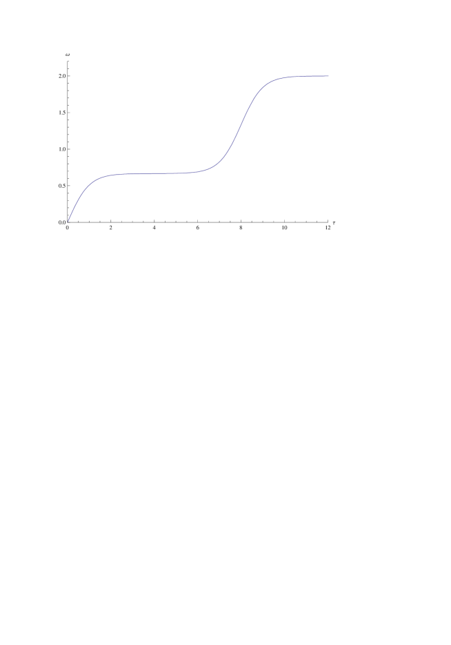
Figure 1: Vorticity $\hat{\omega}(\tau)$ plotted against $\tau$ with saturation value $\hat{\omega}_{c}$=2 and parameter $\tau_{0}$=8.

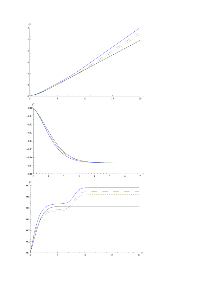
Figure 2: $r=5$, $s=1/5$, $\hat{\omega}_{c}=2$, initial value $\xi_{1}=-\xi_{2}=\xi_{3}=0.1$. Black line ($\hat{\omega}(\tau)=0$, $c_{h}=0$), blue line ($\hat{\omega}(\tau)$ in Fig.1, $c_{h}=0$), dotted line ($\hat{\omega}(\tau)$ in Fig.1, $c_{h}=0.2$) and dash line ($\hat{\omega}(\tau)$ in Fig.1, $c_{h}=0.2$) represents plot I, plot II, plot III and plot IV respectively.

References

• [1] P.Ramaprabhu, G.Dimonte, Yuan-Nan Young, A.C.Calder, B.Fryxell, Phys. Rev. E 74, 066308 (2006).
• [2] V.N.Goncharov, Phys. Rev. Lett. 88, 134502 (2002).
• [3] L.K.Forbes, J. Eng. Mech. 27, 273 (2009).
• [4] Hye-Sook Park, K.T.Lorenz, R.M.Cavallo, S.M.Pollaine, S.T.Prisbrey, R.E.Rudd, R.C.Becker, J.V.Bernier, B.A.Remington, Phys. Rev. Lett. 104,135504 (2010).
• [5] R.Betti, J.Sanz, Phys. Rev. Lett. 97, 205002 (2006).
• [6] M.R.Gupta, L.Mandal, S.Roy, M.Khan, Phys. Plasmas 17, 012306 (2010).
• [7] P.G.Saffman, Vortex Dynamics, Cambridge University Press,(1992).
• [8] Sung-Ik-Sohn, Phys. Rev. E 80, 055303(R) (2009).
• [9] D. Layzer, Astrophys. J. 122, 1 (1955).
Refer to caption