Analytic behavior of the QED polarizability function at finite temperature

Abstract

We revisit the analytical properties of the static quasi-photon polarizability function for an electron gas at finite temperature, in connection with the existence of Friedel oscillations in the potential created by an impurity. In contrast with the zero temperature case, where the polarizability is an analytical function, except for the two branch cuts which are responsible for Friedel oscillations, at finite temperature the corresponding function is not analytical, in spite of becoming continuous everywhere on the complex plane. This effect produces, as a result, the survival of the oscillatory behavior of the potential. We calculate the potential at large distances, and relate the calculation to the non-analytical properties of the polarizability.

I Introduction

The potential created by a static ionic impurity in metallic alloys has been considered by many authors (see, for example FetterWal ; Mahan ). At large distances, the potential shows an oscillatory behavior, damped as negative powers of the distance $r$, a phenomenon which is known as Friedel oscillations FR52 . At zero temperature, this kind of behavior has been associated to the existence of the Kohn singularity KO59 in the quasi-photon polarizability, induced by the sharp edge of the degenerate electron distribution. At the threshold of the interaction, i.e. at the threshold of electron-hole creation, the momentum of the quasi-photon is equal to $2p_{f},$ the diameter of the Fermi sphere, with $p_{f}$ the Fermi momentum of the electrons. It must be noticed that the quasi-photon self-energy presents a singularity at this point. The presence of a singularity allows to obtain, with the help of Lighthill’s method, the asymptotic form ($r\rightarrow\infty$) of the potential, as an expansion in terms of the form $\cos(2p_{f}r)$ and $\sin(2p_{f}r)$, damped as negative powers of $r$, and enhanced by powers of $\log(4p_{f}r)$ LI64 .

Alternatively, one can perform an analytical continuation of the quasi-photon polarizability to complex values of the transferred momentum $q$, and do the integration by deforming the circuit in the complex plane. Aside from the “Debye pole” of the quasi-photon propagator on the imaginary axis, giving an exponentially damped contribution, the polarizability has two branch cuts starting at $q=\pm 2p_{f}$, which are responsible for the long-distance oscillatory behavior FetterWal ; KA88 . In other type of plasmas, one can also find additional complex poles in the propagator, giving raise to an exponentially damped oscillatory contribution SPD01 .

Let us now consider the situation at finite temperature $T$. Since the electron distribution is spread out, from energy and momentum conservation in the collisions between the electrons and soft quasi-photons we expect that screening becomes more effective than in the zero-temperature case. This is, in fact, the case and one obtains that the oscillations are still present, although they are damped as temperature increases FetterWal . Of course, this is a desirable result, showing that the limit $T=0$ is not pathological.

We would like to understand this aspect from a mathematical point of view. On one side, the above discussion, based on the Kohn singularity, does not hold, since we know that the singularity disappears at $T\neq 0$ SPD01 . On the other side, one can be tempted to extend the integration to the complex $q$ -plane. If the $T>0$ polarizability is still an analytical function, one has to face these possibilities: either the function has discontinuities on the complex plane (i.e. branch cuts, as in the $T=0$ case) or poles , or both. As we discuss later, the first possibility does not appear: the polarizability becomes a continuous function at non-zero temperature. On the other hand, the appearance of additional poles, at an arbitrary small temperature, which were not present at $T=0,$ would indicate a strong anomaly, as branch cuts should be suddenly transformed into complex poles, a possibility which looks too exotic and would point towards a singular behavior with temperature. As discussed above, this is not the case. Then, how can we account for the oscillations?

As we show in this paper, the explanation lies on the fact that, at finite temperature, the polarizability is non-analytical over the whole complex plane. In fact, this function can be understood as a superposition of a family of functions, each one having discontinuities at $q=\pm 2p$. Each one of the functions on this family gives an oscillatory result and the sum, for not too large temperatures, is still oscillatory. As temperature increases, the range of values of $p$ that effectively contribute is enlarged, leading to a destructive interference. For this reason, oscillations are damped with temperature.

This paper is organized as follows. The analytical properties of the polarizability function, both at $T=0$ and $T>0$, are discussed in sections 2 and 3. In section 4 an expression for the potential is obtained. Section 5 contains a brief discussion and concluding remarks.

II The polarizability in the complex plane

The potential created by a static ionic impurity in an electron gas can be calculated from:

$$V(r) = \frac{e^{2}}{\pi r}I\left(r\right)$$

$$I\left(r\right) = \int_{-\infty}^{+\infty}dq\,\frac{q\sin(qr)}{\nu(q)}=Im\int_{-\infty}^{+\infty}dq\,\frac{q\exp(iqr)}{\nu(q)},$$ (1)

where

$$\nu(q)=q^{2}-\lambda\chi^{T}(q),$$ (2)

$\lambda=4\pi e^{2}$, $e$ is the electron charge, and $\chi^{T}(q)$ is the polarizability at temperature $T$ within the RPA (random phase approximation), which can be written as:

$$\chi^{T}(q)=\int_{0}^{\infty}dp\,g(p)\chi^{0}(q,p).$$ (3)

Here,

$$\chi^{0}(q,p)=m\frac{-4pq+\left(q^{2}-4p^{2}\right)\log|\frac{q+2p}{q-2p}|}{8\pi^{2}q}$$ (4)

is the $T=0$ polarizability, $m$ is the electron mass, and

$$g(p)=-\frac{\partial f(p)}{\partial p}$$ (5)

where $f$ is the Fermi-Dirac distribution for the electrons

$$f(p)=\frac{1}{1+\exp\left(\frac{\varepsilon\left(p\right)-\mu}{T}\right)}.$$ (6)

We consider a non-relativistic plasma. Therefore, in the latter formula $\varepsilon\left(p\right)=\frac{p^{2}}{2m}$. Finally, $\mu$ is the chemical potential. Under these conditions, we have:

$$g(p)=\frac{p}{4mT}\frac{1}{\left[\cosh\left(\frac{\varepsilon\left(p\right)-\mu}{2T}\right)\right]^{2}}$$ (7)

As mentioned above, Eq. (2) corresponds to the RPA level. A further improvement of this approximation can be introduced via a local field correction. For zero temperature, simple analytical modelizations are given e.g. in ICH82 . However, to our knowledge no such analytical models exist at finite $T$. For this reason, since we only intend to give a qualitative explanation for oscillations at $T>0$, we stay at the RPA level. Of course, in order to obtain more accurate results, one would need to go beyond this approximation.

The usual way to calculate the integral in Eq. (1) is by performing an analytical continuation to the upper complex half-plane:

$$I(r)=Im\int_{C}dq\,\frac{q\exp(iqr)}{\nu(q)},$$ (8)

where $C$ is now a circuit contained on the upper half-plane. In doing so, we need to investigate the analytical properties of $\chi^{T}(q)$ (see Eq. 2) in the interior of $C.$ These properties are defined by Eq. (3).

III Analytical properties of the polarizability function

We start by defining an extension to complex values of $q$ of the function $\chi^{0}$ defined in Eq. (4). Let’s define $\chi^{0}(q,p)$ for $p>0$ and complex $q=x+iy$ by the following formula:

$$\chi^{0}(q,p)=-\frac{mp}{2\pi^{2}}+\frac{m}{8\pi^{2}}\frac{(q-2p)(q+2p)}{q}\left\{\log\frac{|q+2p|}{|q-2p|}+i\left[\arctan\left(\frac{y}{x+2p}\right)-\arctan\left(\frac{y}{x-2p}\right)\right]\right\}.$$ (9)

We first determine a maximal domain in the complex plane where the complex function $\chi^{0}$ is defined. For $p>0$ we define the complex domains $G_{1,p}$, $G_{2,p}$ and $G_{3,p}$ to be respectively the set of all complex $q=x+iy$ such that $\Re q<-2p$, $-2p<\Re q<2p$ and $\Re q<2p$, respectively . One can check that the expression (9) defining $\chi^{0}(q,p)$ converges to $-\frac{mp}{2\pi^{2}}$ as $q\to 0$. We also consider $L$, the principal determination of the complex logarithm

$$L(w)=\log|w|+i\arg w,$$

where $\arg$ is the principal determination to the argument function, taking values between $-\pi$ and $+\pi$. If $q$ is in $G_{1,p}$ we have the following representation:

$$\chi^{0}(q,p)=-\frac{mp}{2\pi^{2}}+\frac{m}{8\pi^{2}}\frac{(q-2p)(q+2p)}{q}\left\{L\left[-\left(q+2p\right)\right]-L\left[-\left(q-2p\right)\right]\right\}.$$

We also have similar representations for $q\neq 0$ in $G_{2,p}$ and in $G_{3,p}$. It follows that $\chi^{0}(q,p)$ is analytic in the domains $G_{p,i}$, excluding perhaps $q=0$ in $G_{p,2}$. Since $\chi^{0}(q,p)$ converges as $q\to 0$, it follows that $\chi^{0}(q,p)$ is analytic on the three domains $G_{p,i}$.

Thus $\chi^{0}(q,p)$ is analytic in the whole complex plane, excluding the two branch cuts $x=\pm 2p$. One can also check that $\chi^{0}$ can be continuously extended to the real points $q=\pm 2p$. It is also true that $\chi^{0}(q,p)$ can be continuously extended to any of the closures $\bar{G}_{p,i}$, but those extensions don’t match up at the boundaries (except at the real points $q=\pm 2p$) since $\chi^{0}$ has jump discontinuities there.

We now consider $\chi^{T}$ defined as in (3) using the complex $\chi^{0}$ instead. In order to prove that the integral defining $\chi^{T}$ exists and to study its analytical properties, (continuity or computation of complex integrals) it is necessary to use the classical theorems of Fubini and Lebesgue from integration theory. The key properties of the function $g(p)$, (7), that will be needed are that $g$ converges to zero exponentially as $p\to\infty$ and that $g(p)=O(p)$ as $p\to 0$. These properties will allow us to dominate products of $g(p)$ and not too fast growing functions of $p$. In particular, if a function $h(p)$ has polynomial growth as $p\to\infty$ and is continuous, or has a behavior like $1/p$ or like $\log p$ as $p\to 0$ , then the product $g(p)h(p)$ will be Lebesgue-integrable and the necessary computations will make sense.

We first consider for which points $q=x+iy$ of the complex plane does the integral in Eq. (3) exist. First of all, since $\chi^{0}(0,p)=-mp/\pi^{2}$, we have that $\chi^{T}(0)$ is well defined by Eq. (3). If we fix a point $q_{0}\neq 0$, formula (9) can be used and we can bound $\chi^{0}(q_{0},p)$ by a polynomial in $p$. In this way, we see that the function $\chi^{T}$ is defined on the whole complex plane.

Turning to the continuity of $\chi^{T}$, we can start with a point $q_{0}\neq 0$ and a sequence $0\neq q_{n}\to q_{0}$. We consider the compact set $K=\{q_{0}\}\cup\{q_{n},n=1,2,\ldots\}$ so that $0\notin K$. We can also use Eq. (9) to obtain a polynomial bound to $|\chi(q,p)|$ uniformly on $q\in K$, so that Lebesgue’s dominated convergence theorem can be applied and the continuity of $\chi^{T}$ at $q_{0}\neq 0$ can be established.

To prove the continuity of $\chi^{T}$ at $q=0$, we bound $\chi^{0}(q,p)$ in a slightly different way. We first consider $q=x+iy$ with $|q|<1$. If $q\in G_{2,p}\setminus\{0\}$, we have

$$\chi^{0}(q,p)=-\frac{mp}{2\pi^{2}}+\frac{m}{8\pi^{2}}(q-2p)(q+2p)\psi_{p}(q,)$$

where

$$\psi_{p}(q)=\frac{L(2p+q)-L(2p-q)}{q},$$

$L$ is the principal determination of the complex logarithm as before, and the function $\psi_{p}$ can be extended to an analytic function in the whole domain $G_{2,p}$. One then checks that

$$\psi_{p}(q)=2L\left(1+\frac{q}{2p}\right).$$

We can check the above equality by expanding both functions in power series for small $\frac{q}{2p}$ and applying analytic continuation to $G_{2,p}$. Then we have the estimate

$$\left|L\left(1+\frac{q}{2p}\right)\right|\leq|\log|2p+q||+|\log 2p|+\frac{\pi}{2},$$

which allow us to bound $|\chi^{0}(q,p)|$ by the sum of a polynomial on $p$ and a term which is the product of a polynomial on $p$ and $|\log 2p|$.

On the other hand, if $q\in G_{1,p}\cup G_{2,p}$, the estimate of $\chi^{0}(q,p)$ as in (9) gives the sum of two terms. The first term involves the logarithmic part of (9) and gives, after some inequalities, a polynomial bound. The second term involves the “arctan” part and, using the fact that $q\in G_{1,p}\cup G_{3,p}$ gives a bound by a polynomial in $p$ multiplied by $1/p$.

In any case, if $|q|<1$, $\chi^{0}(q,p)$ is bounded by terms that are polynomial on $p$, logarithmic or $1/p$, uniformly on $q$. Therefore, the product $g(p)\chi^{0}(q,p)$ is dominated by a Lebesgue-integrable function and $\chi^{T}$ is defined and continuous in the whole complex plane.

Thus, at finite temperature the above mentioned discontinuities disappear, and the function $\chi^{T}(q)$ becomes continuous everywhere. This is clearly illustrated in Fig. 1, where we have plotted the real part of $\chi^{0}(q,p)$ (dashed line). We have chosen $p$ as the Fermi momentum of an electron gas with $r_{s}=3$ , where $r_{s}$ is the mean interelectronic distance in units of the Bohr radius, as usual. We also plot (solid line) the real part of $\chi^{T}(q)$ for the same density, and a temperature $T=0.01T_{F}$ (here, $T_{F}$ is the Fermi temperature). As is apparent from this figure, the discontinuity of $\chi^{0}(q,p)$ around $\Re(q)=2p$ disappears when the temperature is non zero.

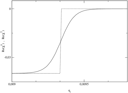
Figure 1: The electron gas polarizability at zero temperature (dashed line), for a value $q_{i}=1$, as a function of $q_{r}$. All magnitudes are in units of the electron mass. For the chosen parameters (see the text), we have $2p=0.00934$ . Also shown for comparison is the finite-temperature polarizability (solid line), when $T=0.01T_{F}$.

It turns out that $\chi^{T}$ is non analytic at any point of the complex plane. To show this, we can compute the integral

$$\int_{R}dq\,\chi^{T}(q)=\int_{R}dq\,\int_{0}^{+\infty}dp\,g(p)\chi^{0}(q,p),$$ (10)

where $R$ is a rectangle. If the rectangle is contained in the first quadrant, standard estimates on $|\chi^{0}(q,p)|$ show that the double integral of $\chi^{0}(q,p)$ is well defined, the needed change of the order of integration is possible, and the usual procedures in complex analysis show that the value of (10) is not zero. The computation can be reproduced in all the other quadrants and we finally arrive to the conclusion that $\chi^{T}$ is not analytic at any point.

We give the details of the computation in the first quadrant as an illustrative example. Suppose that the rectangle $R$ is defined by the vertices $q=x_{0}+iy_{0}$ and $q=x_{1}+iy_{1}$.

We introduce the notations

$$\chi^{0}(C_{2p}^{+}) \equiv \lim_{\epsilon\rightarrow 0}\chi^{0}(2p-\epsilon+iq_{i},p),$$

$$\chi^{0}(C_{2p}^{-}) \equiv \lim_{\epsilon\rightarrow 0}\chi^{0}(2p+\epsilon+iq_{i},p),$$ (11)

and the definition

$$\Delta\chi^{0}(y,p)\equiv\chi^{0}(C_{2p}^{+})-\chi^{0}(C_{2p}^{-})=-\frac{m}{8\pi}\frac{y\left(y-i4p\right)}{\left(y-i2p\right)}.$$ (12)

By deforming the contour integral, we can write

$$\int_{C}dq\,\chi^{0}(q,p)=-i\int_{y_{0}}^{y_{1}}dy\,\Delta\chi^{0}(y,p).$$ (13)

Therefore

$$\int_{R}dq\,\chi^{T}(q)=-i\int_{x_{0}/2}^{x_{1}/2}dp\,g(p)\int_{y_{0}}^{y_{1}}dy\,\Delta\chi^{0}(y,p),$$ (14)

which is different from zero.

IV Computation of the potential

We now return to the computation of $V(r)$, as given by Eq. (8).

First, let us calculate

$$\int_{C}dq\,q\exp(iqr)\chi^{T}(q)=\int_{0}^{\infty}dp\,g(p)\int_{C}dq\,q\exp(iqr)\chi^{0}(q,p),$$ (15)

where $C$ is the contour in figure 2.

In order to see that the above integral is well defined, to be able to interchange the order of integration and to compute the limit when the width of the contours in figure 2 tends to zero, it is necessary to estimate $\chi^{T}(q)$, and take into account that the imaginary part of $q$ in the above contours is unbounded.

We can keep the width of the contours in figure 2 equal to $\epsilon\leq\epsilon_{0}$. Then we can make the estimates for the full rectangles of width $\epsilon_{0}$. It can be checked that the expression $q\exp(iqr)\chi^{0}(q,p)$ admits a polynomial bound in $p$ uniformly on $q$ inside those rectangles if $y\leq|x|$, and that it can be bounded by the product of a polynomial on $p$ by the exponential $\exp(-|q|r/2)$ if $y>|x|$. With those estimates, it can be seen that, defining

$$I(p)=\int_{C}d|q|\,\left|qe^{iqr}g(p)\chi^{0}(q,p)\right|,$$

it follows that $\int_{0}^{+\infty}\d{p}\,I(p)<+\infty$, and the order of integration can be interchanged. Indeed, the expression

$$g(p)\left|\int_{C}dq\,qe^{iqr}\chi^{0}(q,p)\right|$$

can be dominated with a Lebesgue-integrable function of $p$, so that the limit when $\epsilon\to 0$ can be taken inside the integral.

We now compute the value of (15). In the following, we leave aside the contribution from the Debye pole, which lies on the imaginary axis. At zero temperature, its position is given by $q_{D}=\pm i(p_{f}m\lambda)^{1/2}/\pi$. The pole contribution can be easily incorporated in our calculations via the residue theorem, giving rise to an exponentially damped term, which does not appreciably modify the results for the long range behavior we are interested here. Moreover, at finite temperature the pole is located at higher positions on the imaginary axis Ya89 ; Sch02 , therefore giving an even smaller contribution.

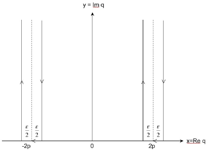
Figure 2: Analytically-continued structure of the zero-temperature polarizability. Represented schematically is the contour path used for integration.

Under this approximation, we can write

$$\int_{C}dq\,q\exp(iqr)\chi^{0}(q,p)$$ (16)

$$= -\left[\begin{array}[]{c}\int_{C_{2p}^{+}}dq\,q\exp(iqr)\chi^{0}(q,p)-\int_{C_{2p}^{-}}dq\,q\exp(iqr)\chi^{0}(q,p)\\ \int_{C_{-2p}^{+}}dq\,q\exp(iqr)\chi^{0}(q,p)-\int_{C_{-2p}^{-}}dq\,q\exp(iqr)\chi^{0}(q,p)dq\end{array}\right]$$ (19)

Let us define, in analogy to Eq. (11)

$$\chi^{0}(C_{-2p}^{+}) \equiv \lim_{\epsilon\rightarrow 0}\chi^{0}(-2p-\epsilon+iq_{i},p)$$

$$\chi^{0}(C_{-2p}^{-}) \equiv \lim_{\epsilon\rightarrow 0}\chi^{0}(-2p+\epsilon+iq_{i},p)$$ (20)

Due to Schwartz’s principle, one has:

$$\chi^{0}(q^{\ast},p)=\left[\chi^{0}(q,p)\right]^{\ast}=\chi^{0}(-q^{\ast},p)$$ (21)

which implies that

$$\chi^{0}(C_{-2p}^{-}) = \left[\chi^{0}(C_{2p}^{+})\right]^{\ast}$$

$$\chi^{0}(C_{-2p}^{+}) = \left[\chi^{0}(C_{2p}^{-})\right]^{\ast}$$ (22)

Substitution on (16) gives, after some algebra

$$\int_{C}dq\,q\exp(iqr)\chi^{0}(q,p)=-2i\int_{0}^{\infty}dp\,\exp(-yr)Re\left[q\exp\left(i2pr\right)\Delta\chi^{0}(y,p)\right]$$ (23)

Therefore

$$\int_{C}dq\,q\exp(iqr)\chi^{T}(q)=-2i\int_{0}^{\infty}dp\,g(p)\int_{0}^{\infty}dy\,\exp(-yr)$$

$$Re\left[(2p+i)\exp\left(i2pr\right)\Delta\chi^{0}(y,p)\right]$$ (24)

By repeating the above procedure, one can obtain the result:

$$\int_{C}dq\,q\exp(iqr)\left[\chi^{T}(q)\right]^{2}=-4i\int_{0}^{\infty}dp\,g(p)\int_{0}^{\infty}dy\,\exp(-yr)$$

$$Re\left[(2p+iy)\exp\left(i2pr\right)\Delta\chi^{0}(y,p)\chi^{T}(2p+iy)\right]$$ (25)

which can be easily generalized to the following formula

$$\int_{C}dq\,q\exp(iqr)\left[\chi^{T}(q)\right]^{n}=-2ni\int_{0}^{\infty}dp\,g(p)\int_{0}^{\infty}dy\,\exp(-yr)$$

$$Re\left[(2p+iy)\exp\left(i2pr\right)\Delta\chi^{0}(y,p)\left[\chi^{T}(2p+iy)\right]^{n-1}\right]$$ (26)

Again, the necessary estimates on the above functions, in order to justify all the steps, can be done in a direct albeit long procedure.

With the help of the previous equations, we can finally proceed with Eq. (1).

$$I(r)=Im\int_{-\infty}^{+\infty}dq\,\frac{q\exp(iqr)}{\nu(q)}=Im\int_{-\infty}^{+\infty}dq\,\frac{q\exp(iqr)}{q^{2}-\lambda\chi^{T}(q)}$$ (27)

To this end, we make an expansion of the denominator in powers of $\lambda$. Using the result of Eq. (26) we obtain, after a straightforward calculation:

$$I(r)=-2\int_{0}^{\infty}dp\,g(p)\int_{0}^{\infty}dy\,\exp(-yr)Re\left[q\exp\left(i2pr\right)\frac{\lambda\Delta\chi^{0}(y,p)}{\nu(q)^{2}}\right]$$ (28)

Here

$$q=2p+iy$$ (29)

We can now use the above result to obtain an approximate expression for $I(r)$ as $r\rightarrow\infty.$ In this case, due to the fast-decaying exponential, is is enough to consider only small values of $y$. To the leading order in $y$ we have, then:

$$\Delta\chi^{0}(y,p) \simeq -\frac{my}{4\pi}$$

$$\nu(2p+iy) \simeq \nu(2p)$$ (30)

and one easily obtains

$$I(r)\simeq\frac{\lambda m}{\pi r^{2}}\int_{0}^{\infty}dp\,g(p)\frac{p\cos(2pr)}{\nu(2p)^{2}}$$ (31)

This formula is valid, for an arbitrary temperature, at sufficiently large distances and is specially suited, in contrast to the initial expression Eq. (1), to low temperatures. Indeed, as $T\rightarrow 0$ the function $g(p)$ is strongly peaked around the Fermi momentum $p_{F}$ and allows for a fast convergence in the above expression. Within this limit, therefore, we can make further approximations, namely:

$$I(r)\simeq\frac{\lambda m}{\pi r^{2}}\frac{p_{F}}{\nu(2p_{F})^{2}}\int_{0}^{\infty}dp\,g(p)\cos(2pr)$$ (32)

After some algebra, one arrives to the final result

$$V(r)\simeq 8\frac{e^{4}}{r^{2}}\frac{m^{2}T}{\nu(2p_{F})^{2}}\frac{\cos(2p_{F}r)}{\sinh\left(\frac{2\pi mTr}{p_{F}}\right)}$$ (33)

In this way, we have obtained an oscillatory behavior for $V(r)$ at finite temperature. Whenever $\frac{2\pi mTr}{p_{F}}\gg 1,$ one can approximate $\sinh\left(\frac{2\pi mTr}{p_{F}}\right)\simeq\frac{1}{2}\exp\left(\frac{2\pi mTr}{p_{F}}\right),$ giving raise to an exponential suppression of Friedel oscillations at finite temperature. This is a very well-known result, which can be obtained using e.g. some modification of Lighthill’s method to finite temperature (see, for example DPS89 ; DGP94 ). Such methods, however, immediately raise the question of what the possible origin of the oscillations is, as discussed in the introduction. Our method is based on the integration of $\chi^{0}(q,p)$ on the complex plane, by interchanging the limits of integration (see (15)). In the next section we give an intuitive description of this procedure, leading to (33).

V Discussion

In this paper, we have revisited the method to obtain the screened potential on an electron gas at finite temperature using the properties of the zero-temperature polarizability. We analyzed with detail the mathematical properties of this function on the complex plane. The formula we obtained for the potential in the low-temperature regime coincides with previous results in the literature, giving an oscillatory function, which is damped as temperature increases. The existence of oscillations at non-zero, but sufficiently low temperatures, shows that the limit $T\rightarrow 0$ is smoothly reached in the model, and does not represent a pathology. However, the explanation based on the Kohn singularity fails to account for the persistence of the oscillations. In fact, the electron distribution is smeared out over a range of the order $\sim T$ in energies, and therefore the Kohn singularity disappears. On the other hand, for $T>0$ the function $\chi^{T}(q)$ becomes continuous, so that the argument we used at zero temperature does not apply to explain Friedel oscillations at finite temperature.

In fact, as we have learned from the previous section, the function $\chi^{T}(q)$ is non-analytical everywhere on the complex plane. From an intuitive point of view, we can regard Eq. (3) as a superposition of a family (as $p$ varies) of functions $\chi^{0}(q,p),$ each one having discontinuities at $q=\pm 2p$. This sum is spread out, due to the weight function $g(p)$, over a range $\sim T$ in energies. By interchanging the order of the integration, as in (15), we obtain a superposition of oscillatory terms, Eq. (32), which results in (33).

In our calculations, we have considered only a qualitative discussion based on the RPA. It would be interesting to go beyond this approximation, by introducing a local field correction. Unfortunately, to our knowledge, there is no analytical formula which accounts for these effects in the case of finite temperature.

- (1) A. L. Fetter and J. D. Walecka, Quantum Theory of Many-Particle Systems (McGraw-Hill, Inc., 1971)
- (2) G. D. Mahan, ”Many-particle physics”. Plenum Press, New York, (1981).
- (3) J. Friedel, Phyl. Mag. 43 (1952), 153. Nuovo Cim. 7 (1958), Suppl.2 287.
- (4) W. Kohn, Phys. Rev. Lett. 2 (1959) 393.
- (5) M.J. Lighthill, ”Introduction to Fourier Analysis and Generalized Functions” (Cambridge Univ. Press, Cambridge 1964).
- (6) J. Kapusta, T. Toimela, Phys. Rev. D37 (1988) 3731.
- (7) H. Sivak, , A. Pérez and Joaquín Díaz Alonso. Prog. in Th. Phys. 105 (2001) 961-978. hep-ph/9803344.
- (8) S. Ichimaru, Rev. Mod. Phys. 54 (1982) 1017.
- (9) H. Yamada, Phys. Lett. B 223 (1989) 229.
- (10) R. A. Schneider, Phys. Rev. D 66 (2002) 036003.
- (11) J. Diaz Alonso, A. Pérez and H. Sivak, Nucl. Phys. A205 (1989) 695.
- (12) J. Diaz Alonso, E. Gallego, A. Pérez Phys. Rev. Lett. V73 N19 (1994) 2536.