Spectral lag of gamma-ray burst caused by the intrinsic spectral evolution and the curvature effect

Abstract

Assuming an intrinsic ‘Band’ shape spectrum and an intrinsic energy-independent emission profile we have investigated the connection between the evolution of the rest-frame spectral parameters and the spectral lags measured in gamma-ray burst (GRB) pulses by using a pulse model. We first focus our attention on the evolution of the peak energy, $E_{0,p}$, and neglect the effect of the curvature effect. It is found that the evolution of $E_{0,p}$ alone can produce the observed lags. When $E_{0,p}$ varies from hard to soft only the positive lags can be observed. The negative lags would occur in the case of $E_{0,p}$ varying from soft to hard. When the evolution of $E_{0,p}$ and the low-energy spectral index $\alpha_{0}$ varying from soft to hard then to soft we can find the aforesaid two sorts of lags. We then examine the combined case of the spectral evolution and the curvature effect of fireball and find the observed spectral lags would increase. A sample including 15 single pulses whose spectral evolution follows hard to soft has been investigated. All the lags of these pulses are positive, which is in good agreement with our theoretical predictions. Our analysis shows that only the intrinsic spectral evolution can produce the spectral lags and the observed lags should be contributed by the intrinsic spectral evolution and the curvature effect. But it is still unclear what cause the spectral evolution.

1 Introduction

The phenomenon of the observed spectral lag of Gamma-ray burst (GRB) is very common. Since Cheng et al. (1995) first analyzed the spectral lags of GRBs based on BATSE Large Area Detector channel 1 (25-50 keV) and channel 3 (100-300 keV) light curves, several authors have carried out more analysis work on the GRB lags (e.g., Norris et al., 2000; Wu & Fenimore 2000; Chen et al. 2005; Yi et al. 2006; Peng et al. 2007).

Several attempts to explain the origin of the spectral lag have been put forward. The dominant behavior observed in GRBs, positive lags, is that the soft radiation lagging the hard, can be produced by several reasons. An intrinsic cooling of the radiating electrons cause the radiation to dominate at lower energies. A Compton reflection of a medium at a sufficient distance from the initial hard source will also cause a positive lag. While the photons emit at relativistic speeds from different latitudes of a convex surface (the curvature effect) will cause the radiation to be delayed and softened, thus producing a observed positive lag (e.g., Qin 2002; Ryde & Petrosian 2002; Qin et al. 2004; Shen et al. 2005). The negative lag is defined as the hard radiation lagging behind the soft. However, few attempts are made to explain the origin of the negative lag. The possible scenario is a hot medium, say a lepton cloud surrounding a cooler emitter, which will cause the soft radiation to be upscattered by inverse Comptonization. The photons get harder the more scatterings they suffer and thus they are more delayed. A definitive explanation of the origin of them has not yet been given. The origin of the spectral lags are still unclear.

Kocevski & Liang (2003) pointed out that the observed lag is the direct result of spectral evolution. They measured the rate of $E_{p}$ decay ($\Phi_{0}$) for a sample of clean single-peaked bursts with measured lag and used this data to provide an empirical relation that expresses the GRB lag as a function of the burst’s spectral evolution rate. While the studies of GRB spectra have shown that GRB spectral evolution is a common phenomenon (e.g.,, Kargatis et al. 1994; crider et al. 1997; Band 1997; Kaneko et al. 2006; Butler & Kocevski 2007).

Recently, Shen et al. (2005) tentatively studied the contribution of curvature effect of fireball to the lag, and the resulting lags are very closed to the observed one. Lu et al. (2006) also studied the spectral lags more detailed based on Doppler effect of fireball (or in some papers, the curvature effect) (see, Qin 2002; Qin et al. 2004; Peng et al. 2006 for more detailed description) and confirmed that the curvature effect can produce the observed spectral lags. They performed more precise calculation with both formulae presented by Shen et al. (2005) and Qin et al. (2004). Some conclusions obtained by Shen et al. (2005) were ascertained, and more complete conclusions on spectral lags resulting from curvature effect were obtained. Lu et al. (2006) argued that, as long as the whole fireball surface is concerned, both formulas were identical in the case of ultra-relativistic motions. Other cases did not study by Shen et al. (2005) were investigated by Lu et al. (2006) and some new conclusions were drawn. These seem show that the curvature effect can indeed produce the spectral lags. In addition, several studies show that the curvature effect also plays an important role in the early X-ray afterglow of GRBs where the so-called softening phenomenon is observed (Qin 2008a, 2008b; Qin 2009).

As pointed out above that the fundamental origin of the observed lag is the evolution of the GRB spectra and the curvature effect can produce the observed lags. Moreover it is mentioned clearly that whilst the curvature effect can account for the main part of the hardness ratio curves of the GRBs concerned and an intrinsic spectral evolution is required to fully explain the observed data (Qin et al. 2006). These motivate our investigations below. How the influences of intrinsic spectral evolution on the spectral lags are when the curvature effect plays an important role or does not? Can the negative lags be produced in the course of intrinsic spectral evolution? We introduce the theoretical formula of the GRB pulse in Section 2. Various possible cases of producing the spectral lags when neglect the curvature effect are studied in Section 3. In Section 4 we investigate the lags when spectral evolution and curvature effect take effect simultaneously. We employ a sample to test the prediction in Section 5. In the last section, we give the conclusions and discussion.

2 Theoretical formula

The observed gamma-ray pulses are believed to be produced in a relativistically expanding and collimated fireball because of the large energies and the short time-scales involved. To account for the observed pulses and spectra of bursts, the Doppler effect (or curvature effect in some paper) over the whole fireball surface would play an important role (e.g., Meszaros and Rees 1998; Hailey et al. 1999; Qin 2002; Qin et al. 2004). The Doppler effect is the photons emitted from the region on the line of sight and those off the line of sight an angle of $\theta$ are Doppler-boosted by different factors and travel different distances to the observer. Therefore, we adopt the model derived by Qin (2002) and Qin et al. (2004) to explore the spectral lags. But our attention is concentrated on the case of $\theta\simeq$0. The count rate within energy channel $[\nu_{1},\nu_{2}]$ is rewritten as formula (1).

$$\begin{array}[]{l}C(\tau)=[2\pi R_{c}^{3}\int_{\widetilde{\tau}_{\theta,\min}}^{\widetilde{\tau}_{\theta,\max}}\widetilde{I}(\tau_{\theta})(1+\beta\tau_{\theta})^{2}(1-\tau+\tau_{\theta})d\tau_{\theta}\\ \times\int_{\nu_{1}}^{\nu_{2}}\frac{g_{0,\nu}(\nu_{0,\theta})}{\nu}d\nu]\times[hcD^{2}\Gamma^{3}(1-\beta)^{2}(1+\frac{\beta}{1-\beta}\tau)^{2}]^{-1}\end{array}$$ (1)

where the $\tau_{\theta}$ is dimensionless relative local time defined by $\tau_{\theta}\equiv c(t_{\theta}-t_{c})/R_{c}$, $t_{\theta}$ is the emission time in the observer frame, called local time, of photons emitted from the concerned differential surface $ds_{\theta}$ of the fireball ($\theta$ is the angle to the line of sight), $t_{c}$ is the initial local time which could be assigned to any values of $t_{\theta}$, and $R_{c}$ is the radius of the fireball measured at $t_{\theta}=t_{c}$. Variable $\tau$ is a dimensionless relative observation time defined by $\tau\equiv[c(t-t_{c})-D+R_{c}]/R_{c}$, where $D$ is the distance of the fireball to the observer, and $t$ is the observation time measured by the distant observer.

In formula (1), $\widetilde{I}(\tau_{\theta})$ represents the development of the intensity magnitude of radiation in the observer frame, called as a local pulse function, and $g_{0,\nu}(\nu_{0,\theta})$ describes the rest-frame radiation mechanisms.

For the sake of simplicity we first adopt Gaussian pulse as rest-frame local pulse. As for the rest-frame radiation spectrum we employ the most frequently used Band function (Band et al. 1993) since it is rather successfully employed to fit the spectra of the GRBs. The two forms are rewritten as formulas (2) and (3).

$$\widetilde{I}(\tau_{\theta})=I_{0}\exp[-(\frac{\tau_{\theta}-\tau_{\theta,0}}{\sigma})^{2}]\qquad(\tau_{\theta,\min}\leq\tau_{\theta}),$$ (2)

$$g_{0,\nu}(\nu_{0,\theta})=\left\{\begin{array}[]{c}(\frac{\nu_{0,\theta}}{\nu_{0,p}})^{1+\alpha_{0}}\exp[-(2+\alpha_{0})\frac{\nu_{0,\theta}}{\nu_{0,p}}],\\ \qquad\quad(\frac{\nu_{0,\theta}}{\nu_{0,p}}<\frac{\alpha_{0}-\beta_{0}}{2+\alpha_{0}})\\ (\frac{\alpha_{0}-\beta_{0}}{2+\alpha_{0}})^{\alpha_{0}-\beta_{0}}\exp(\beta_{0}-\alpha_{0})(\frac{\nu_{0,\theta}}{\nu_{0,p}})^{1+\beta_{0}}\\ \qquad(\frac{\nu_{0,\theta}}{\nu_{0,p}}\geq\frac{\alpha_{0}-\beta_{0}}{2+\alpha_{0}}),\\ \end{array}\right.$$ (3)

where $I_{0}$, $\sigma$ and $\tau_{\theta,min}$ are constants, $\alpha_{0}$ and $\beta_{0}$ are the low- and high-energy indices in the rest frame, respectively, and $\nu_{0,p}$ is the rest-frame peak frequency.

Light curves determined by formula (1) are dependent on the integral limits $\widetilde{\tau}_{\theta,\min}$ and $\widetilde{\tau}_{\theta,\max}$, which are determined by the concerned area of the fireball surface, together with the emission ranges of the radiated frequency and the local time. The integral limits are only determined by

$$\left\{\begin{array}[]{c}\widetilde{\tau}_{\theta,\min}=\max\{\tau_{\theta,\min},{\frac{\tau-1+\cos\theta_{\max}}{1-\beta\cos\theta_{\max}}}\}\\ \widetilde{\tau}_{\theta,\max}=\min\{\tau_{\theta,\max},\frac{\tau-1+\cos\theta_{\min}}{(1-\beta\cos\theta_{\min}}\},\end{array}\right.$$ (4)

where $\tau_{\theta,\min}$ and $\tau_{\theta,\max}$ are the lower and upper limit of $\tau_{\theta}$ confining $\widetilde{I}(\tau_{\theta})$, and $\theta_{\min}$ and $\theta_{\max}$ are confined by the concerned area of the fireball surface. The radiations are observable within the range of

$$\begin{array}[]{c}(1-\cos\theta_{\min})+(1-\beta\cos\theta_{\min})\tau_{\theta,\min}\leq\tau\leq\\ (1-\cos\theta_{\max})+(1-\beta\cos\theta_{\max})\tau_{\theta,\max}\end{array}$$ (5)

Due to the constraint to the lower limit of $\tau_{\theta}$, which is $\tau_{\theta,min}>-1/\beta$ (see, Qin et al. 2004), we assign $\tau_{\theta,0}=10\sigma+\tau_{\theta,min}$ so that the interval between $\tau_{\theta,min}$ and $\tau_{\theta,0}$ would be large enough to make the rising phase of the local pulse close to that of the Gaussian pulse. From formula (2) one can obtain

$$\Delta\tau_{\theta,FWHM}=2\sqrt{ln2}\sigma,$$ (6)

which leads to

$$\sigma=\Delta\tau_{\theta,FWHM}/2\sqrt{ln2},$$ (7)

where $\Delta\tau_{\theta,FWHM}$ is the $FWHM$ (full width at half maximum) of the Gaussian pulse. From the relation between $\tau_{\theta}$ and $t_{\theta}$, one gets

$$\Delta t_{\theta,FWHM}=(R_{c}/c)\Delta\tau_{\theta,FWHM}.$$ (8)

In the following sections, we assign $(2\pi R_{c}^{3}I_{0})/(hcD^{2})$=1, $R_{c}=3\times 10^{15}$ cm, $\tau_{\theta,min}$= 0 .

Because peak times of different light curves associated with different frequency intervals $[\nu_{1},\nu_{2}]$ or different energy bands $[E_{1},E_{2}]$ are different, following Shen et al. (2005) and Lu et al. (2006), we define the spectral lags as the differences between the pulse peak times in two different energy channels, a lower energy channel $[E_{1},E_{2}]$ and a higher energy channel $[E_{3},E_{4}]$. In the following analysis we only consider the energy channel pair: BATSE channels 1 (25–50 keV) and 3 (100–300 keV) which we denote the lag as $lag_{13}$ since it was investigated by most of authors (e.g., Norris et al. 2000; Chen et al. 2005).

3 Spectral lags caused by the spectral evolution alone

Since Kocevski & Liang (2003) pointed out that the observed lag is the result of spectral evolution, let us first investigate the spectral lags due to the spectral evolution alone. That is we consider the radiations emitted from a very small area with $\theta_{min}=0$ and $\theta_{max}=10^{-5}\times 1/\Gamma$ where the photons emitted travel almost same distances to the observer. In this case we think that the curvature effect has no role on the producing of spectral lag.

Observations show that the spectral parameters of the GRBs vary with time. In addition, the parameters of the Band function low- and high-energy indices $\alpha$, $\beta$ and the peak energy of GRB’s $\nu F_{\nu}$ spectrum $E_{p}$ in the observed frame are mainly distributed within $-1.5$ — $-0.5$, $-3.2$ — $-2.1$ and 100 — 700 keV and their typical values are $\alpha=-1$ and $\beta=-2.25$, $E_{p}=250$ keV, respectively (Preece et al. 1998, 2000; Kaneko et al. 2006). Qin (2002) showed the Doppler effect can not affect the intrinsic spectral shapes. When we take the Doppler effect of fireballs into account, the observed peak energy would be related to the peak energy of the rest-frame Band function spectrum ($\alpha_{0}=\alpha$, $\beta_{0}=\beta$) by $E_{p}\simeq 1.67\Gamma E_{0,p}$ (see, Table 4 in Qin 2002). In the following we first consider the common evolutionary model of the rest-frame spectral parameters to investigate the spectral lags. Then the other possible cases are also taken into account.

3.1 Spectral lags of the rest-frame spectral parameters remain constant

We first explore if the spectral lags would occur when the rest-frame spectral parameters remain unchanged to check the effect of spectral evolution on the spectral lag. The typical values of the low- and high-energy indices $\alpha_{0}=-1$ and $\beta_{0}=-2.25$ and $E_{0,p}=250/1.67\Gamma$ keV are taken. Here we assign the $\sigma=1.0$ and take $\Gamma$ = 100, 200, 300, 400, 500, 600, 700, 800, 900, 1000, respectively since the Lorentz factor of fireball are generally larger than 100. We find that all the spectral lags $lag_{13}$ in this case are 0. This suggests that there has no spectral lags when the rest-frame spectral parameters are constant and the curvature effect does not play a role on the spectral lag. Fig. 1 (panel (a)) gives a example plot for this case. The lines of the peak times of the two pulses are superposed each other.

Figure 1: Example light curves of the Band spectral parameters $E_{0,p}$ remain unchanged (a), the $E_{0,p}$ varying from hard to soft (b) and soft to hard (c), where the solid and dashed curves represent the light curves of BATSE channels 1 and 3, respectively.

3.2 Spectral lags of the rest-frame spectral parameters varying from hard to soft

Many investigations of the spectra of GRB show that the spectral softening is an universal phenomenon. In addition, Koceviski and Liang (2003) pointed out as the $E_{p}$ of $\nu F_{\nu}$ spectra decays through the four BATSE channels and produce what we measure as lag. Schaefer (2004) found that only the evolution of $E_{p}$ can produce observed lag using the general Liang-Kargatis relation (which describes how the peak photon energy in the spectrum changes with time). Therefore, we first investigate the case of $E_{p}$ in the rest-frame varying from hard to soft. Following Qin et al. (2005), we assume a simple evolution of the peak energy $E_{0,p}$, which follows $\log E_{0,p}=0.1-k(\tau_{\theta}-\tau_{\theta,1})/(\tau_{\theta,2}-\tau_{\theta,1})$ $(keV)$ for $\tau_{\theta,1}\leq\tau_{\theta}\leq\tau_{\theta,2}$. For $\tau_{\theta}<\tau_{\theta,1}$, $\log E_{0,p}=0.1$ $(keV)$, while for $\tau_{\theta}>\tau_{\theta,2}$, $\log E_{0,p}=0.1-k$ $(keV)$.

Here we also take $\Gamma$ = 100, 200, 300, 400, 500, 600, 700, 800, 900, 1000, respectively and $\alpha_{0}=-1$, $\beta_{0}=-2.25$, $\sigma=1.0$ are assigned. For each $\Gamma$ we assume $k=$ 0.1, 0.2, 0.3, 0.4, 0.5, 0.6, 0.7, 0.8, 0.9, 1.0, 1.1, 1.2, 1.3 and 1.4 (they correspond to different rates of decreasing) to investigate the spectral lag’s dependence.

The local Gaussian pulse (see equation (2)) is employed to study this issue. We adopt $\tau_{\theta,1}=8\sigma+\tau_{\theta,min}$, $\tau_{\theta,2}=12\sigma+\tau_{\theta,min}$ and $\tau_{\theta,0}=10\sigma+\tau_{\theta,min}$.

In this way, we can compute the spectral lags. It is found that all of the lags are positive. A example light curve is showed in Fig. 1 (panel (b)), which illustrates the connection between the spectral evolution and the spectral lag. This indicates the maximum of the photon count rates at the higher energy arrives earlier than at the lower energy in the case of hard-to-soft. Therefore, we can deduce that only hard-to-soft spectral evolution can produce the positive spectral lags.

3.3 Spectral lags of the rest-frame radiation form varying from soft to hard with time

Band (1997) found that a small fraction of GRB spectra ($\sim$ 10%) vary from soft to hard with time. Kargatis et al. (1994) also found this case. Therefore, we also investigate the case of the rest-frame radiation form varying from soft to hard. We also assume a simple case that the evolution of peak energy $E_{0,p}$ follows: $\log E_{0,p}=-0.8+k(\tau_{\theta}-\tau_{\theta,1})/(\tau_{\theta,2}-\tau_{\theta,1})$ $(keV)$ for $\tau_{\theta,1}\leq\tau_{\theta}\leq\tau_{\theta,2}$. For $\tau_{\theta}<\tau_{\theta,1}$, and $\log E_{0,p}=-0.8$ $(keV)$, while for $\tau_{\theta}>\tau_{\theta,2}$, $\log E_{0,p}=-0.8+k$ $(keV)$. The $\Gamma$, $k$, $\alpha_{0}$ and $\beta_{0}$ are taken the same values as the case of hard-to-soft. We also adopt $\tau_{\theta,1}=8\sigma+\tau_{\theta,min}$, $\tau_{\theta,2}=12\sigma+\tau_{\theta,min}$ and $\tau_{\theta,0}=10\sigma+\tau_{\theta,min}$.

According to our computation the soft-to-hard spectral evolution can result in the negative spectral lags alone. Fig. 1 (panel (c)) also demonstrates two example light curves indicating the connection between the spectral evolution and the spectral lag in the case of the rest-frame radiation form varying from soft to hard with time.

3.4 Spectral lags of the rest-frame radiation form varying from soft to hard then to soft

As several authors pointed out that the evolution of the low-energy index $\alpha$ and $E_{p}$ exhibit the “tracking” (the observed spectral parameters follow the same pattern as the flux or count rate time profile, i.e. the evolution of spectral parameters exhibit soft-to-hard-to-soft) behaviors (e.g., Ford et al. 1995; Crider et al. 1997; and Kaneko et al. 2006; Peng et al. 2009a, 2009b). So we investigate the case of $E_{0,p}$ varying from soft to hard then to soft. In order to ensure that the three parameters are in the range of observed values we adopted the following evolutionary form: $\log E_{0,p}=-0.8+k1(\tau_{\theta}-\tau_{\theta,1})/(\tau_{\theta,0}-\tau_{\theta,1})$ $(keV)$ for $\tau_{\theta,1}\leq\tau_{\theta}\leq\tau_{\theta,0}$, $\log E_{0,p}=-0.8+k1-k2(\tau_{\theta}-\tau_{\theta,0})/(\tau_{\theta,2}-\tau_{\theta,0})$ $(keV)$ for $\tau_{\theta,0}\leq\tau_{\theta}\leq\tau_{\theta,2}$, $\log E_{0,p}=-0.8+k1-k2$ $(keV)$ for $\tau_{\theta}>\tau_{\theta,2}$, while for $\tau_{\theta}<\tau_{\theta,1}$, $\log E_{0,p}=-0.8$ $(keV)$. where the k1 and k2 denote the increasing rate of soft-to-hard phase and the decreasing rate of hard-to-soft phase, respectively. We take $\Gamma=$ 100, 200, 300, 400, 500, 600, 700, 800, 900, 1000, respectively and $k1=$ 0.3, 0.4, 0.5, 0.6, 0.7, 0.8, 0.9, 1.0, and 1.1, $k2=$ 0.1, 0.2, 0.3, 0.4, 0.5, 0.6, 0.7, and 0.8, respectively. We also adopt $\tau_{\theta,1}=8\sigma+\tau_{\theta,min}$, $\tau_{\theta,2}=12\sigma+\tau_{\theta,min}$ and $\tau_{\theta,0}=10\sigma+\tau_{\theta,min}$.

We use this form to investigate the spectral lags and find that the negative lag disappears. We explore $E_{0,p}$ and $\alpha_{0}$ varying from soft to hard then to soft. The same form as $E_{0,p}$ is also adopted for $\alpha_{0}$. We find there are negative spectral lags in this case but it does not occur in the small $\Gamma=$100. When the $\Gamma$ is larger than 100, the negative lags will come into being only in the case of the differences between k1 and k2 coming to at least 0.5. That is if the increasing rate of soft to hard is larger than the decreasing rate of hard to soft by at least 0.5 the negative lags would occur. As the increasing of $\Gamma$ the difference needed would decrease. The above assumption is reasonable for the tracking pulse because it is consistent with the result of the hardness evolutionary characteristics of the tracking pulses investigated by Peng et al. (2009a) that the duration of the rise phase are much shorter than that of the decay phase. Fig. 2 illustrates four example light curves.

Figure 2: Example light curves of the negative (left panel) and positive (right panel) spectral lags for the case of soft-to-hard-to-soft, where the symbols are the same as those adopted in Fig. 1.

3.5 Spectral lags of a suddenly shining and gradually dimming intrinsic emission profile

If the different intrinsic emission profiles are different in producing the spectral lags. Similar to Qin et al. (2004) and Shen et al. (2005) we also consider the one-sided exponential decay and power-law decay profile, which are listed as follows, respectively:

$$\widetilde{I}(\tau_{\theta})=I_{0}\exp[-(\frac{\tau_{\theta}-\tau_{\theta,\min}}{\sigma})]\qquad(\tau_{\theta,\min}\leq\tau_{\theta}),$$ (9)

$$\widetilde{I}(\tau_{\theta})=I_{0}(1-\frac{\tau_{\theta}-\tau_{\theta,\min}}{\tau_{\theta,\max}-\tau_{\theta,\min}})^{\mu}\qquad(\tau_{\theta,\min}\leq\tau_{\theta}),$$ (10)

We assume the $\tau_{\theta,\min}$ = 0 and $\mu$ = 2 in the following analysis. The hard-to-soft and soft-to-hard spectral evolution are investigated to check if the two sorts of local pulses also result in the same results as those of the Gaussian pulses. The same evolutional patterns adopted above are employed to explore this issue. We find the results are in agreement with that of Gaussian local pulses. The example plots in Figs. 3 and 4 also illustrate the connection between the spectral evolution and spectral lag for the exponential decay and power-law decay, respectively. This suggests the intrinsic emission profile has no effect on the connection between the spectral evolution and the spectral lags. Likewise, the hard-to-soft evolution produces positive lags and the soft-to-hard evolution leads to negative lags if we adopt other rest-frame local pulses.

Figure 3: Example light curve of $E_{0,p}$ varies from hard to soft (left panel) and soft to hard (right panel) for the case of the exponential decay local pulse, where the symbols are the same as those adopted in Fig. 1.

Figure 4: Example light curve of $E_{0,p}$ varies from hard to soft (left panel) and soft to hard (right panel) for the case of power law decay local pulses, where the symbols are the same as those adopted in Fig. 1.

4 Spectral lags caused by the spectral evolution and the curvature effect

As previous section pointed out that the curvature effect must be play a role on the producing of temporal and spectral profile we also take the effect into account to study the spectral lag. The evolutionary form, hard-to-soft and soft-to-hard, are combined with curvature effect to explore the influence of the combined effects on the spectral lags. That is we consider the radiation emitted from a big area with $\theta_{min}=0$ and $\theta_{max}=\pi/2$ where the photons emitted travel different distances to the observer. The photons on the line of sight arrive at us earlier than that of off sightline. In this way the lags due to curvature effect is always positive and the hard-to-soft evolution also make the lag is positive. Therefore we think the spectral lags caused by the combined effect must be increase.

We first consider the case of $E_{0,p}$ varying from hard to soft combined with the curvature effect. In addition, we also assume the evolution of $E_{0,p}$ follows the same means as the above section. To compare the lags produced by the spectral evolution alone with that by the spectral evolution and curvature effect together we plot two sorts of lags together in Fig. 5 (panel (a)) by considering a set of parameter values. Note that the histogram plots may mean nothing because when one consider another set of parameter values they get a different result. It is shown that (i) the average value of spectral lags caused by spectral evolution and combined effect are 0.1086 s and 0.1692 s, respectively and (ii) the corresponding medians are 0.007 s and 0.016 s, respectively. These show the lags caused by the combined effect increase indeed. Whether the curvature effect also make the lags increase in the case of soft-to-hard or not? We also check the spectral lags resulting from the curvature effect and evolution of $E_{0,p}$ following soft-to-hard. The lags produced by spectral evolution alone and the combined effect are also compared. The mean values are -0.1200 s and -0.0114 s for spectral evolution and combined effect, respectively. Whereas the corresponding median values are -0.0102 s and -0.0005 s, respectively. Fig. 5 (panel (b)) also shows that the lags indeed increase in the case of soft-to-hard. In addition, we also find due to the curvature effect some negative lags change into positive ones. In view of the analysis of the above two cases we can conclude that the curvature effect indeed make the lags increase significantly.

Figure 5: The comparisons of lag distribution between the case of hard-to-soft (panel a) and soft-to-hard (panel b) evolution alone (solid lines) and the case of spectral evolution and curvature effect simultaneously (the dashed lines).

5 Observed spectral lags of the hard-to-soft pulses

The above analysis shows that the spectral lags resulting from the hard-to-soft spectral evolution are positive and the negative lags may come from the soft-to-hard or soft-to-hard-to-soft spectral evolution. We wonder if the observations are consistent with the predictions. The pulses exhibit hard-to-soft, soft-to-hard and soft-to-hard-to-soft spectral evolution should be checked. However, the spectral parameter evolution of observed pulses generally exhibit hard-to-soft and “tracking” (i.e. soft-to-hard-to-soft). Both behaviors are defined by $E_{p}$ and/or low-energy index evolution, which are found by several authors (Kaneko et al. 2006; Ford et al. 1995; Crider et al. 1997). With ordinary Poisson noise in GRB light curves, there will be significant scatter in the measured lags. The percentage of lags increase substantially towards small values, with many (the high luminosity events) having near-zero lags. In such a case, we expect there to be many “measured” negative lags, even if all lags are positive-definite. That is, a convolution of a positive-definite lag distribution with the known measurement errors apparently reproduces the observed lag distribution including the measured negative lags. With this, a good case can be made that negative lags do not exist. The existence of multiple overlapping pulses could easily produce negative lags, even though the lags for each pulse are positive. All it takes is two nearly overlapping pulses with the second one being harder than the first. In all, we are not convinced in the significant existence of negative lags.

Therefore, we select a sample only containing the FRED (fast rise and exponential decay) pulses provided by Kocevski et al. (2003) to check the theoretical predication since these bursts exhibit clean, single-peaked or well-separated in multi-peaked events. We can obtain directly the spectral parameters of bright bursts from Kaneko et al. (2006). The weaker bursts are also analyzed using RMFIT software and fitted with Band model. Similar to Peng et al. (2009a, 2009b, 2010) and Ryde & Svensson (2002) a signal-to-noise ratio (S/N) of the observations of at least $\geq$ 30 to get higher time resolution are adopted. For the hard-to-soft pulses only that containing at least 1 data points of $E_{p}$ before the peak time of pulse and 4 in all are included in the our analysis. Finally, we select 15 hard-to-soft pulses as our sample to test our predictions. Illustrated in Fig. 6 are the spectral and temporal behaviors for our sample.

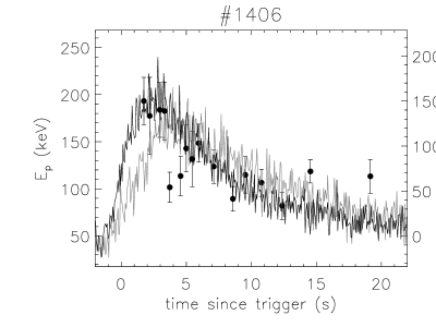
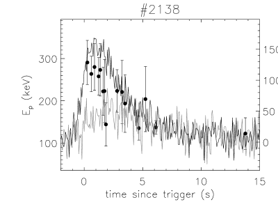
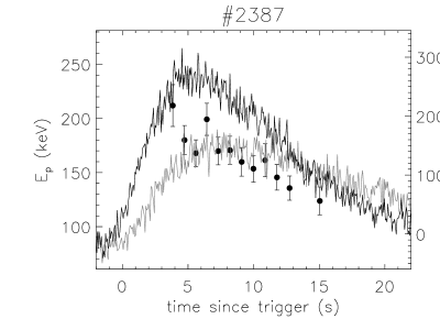
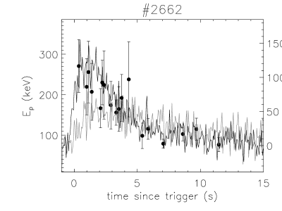
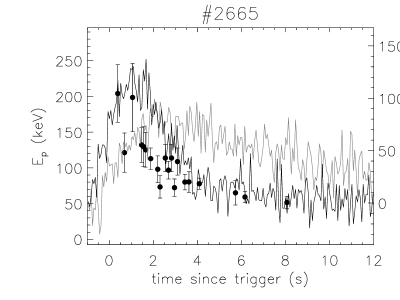
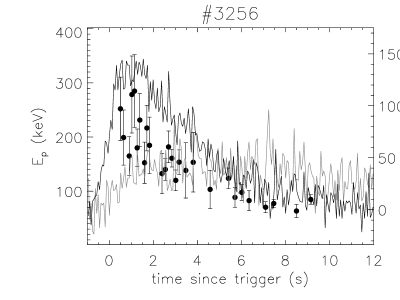
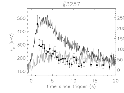
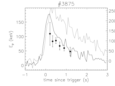
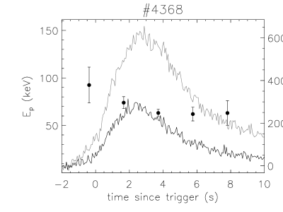
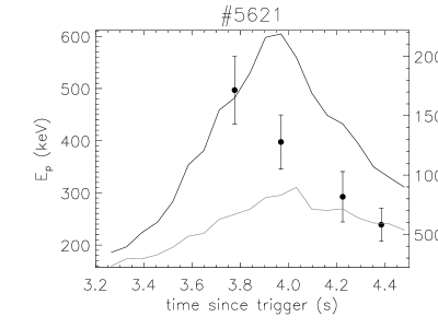
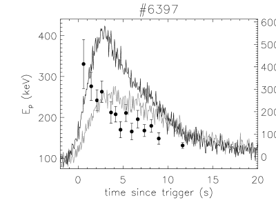
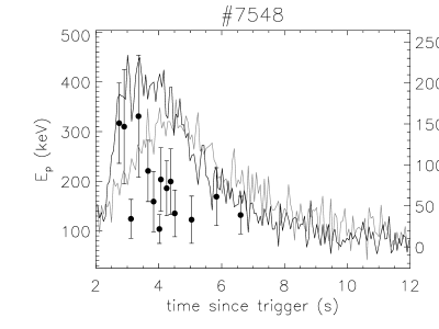
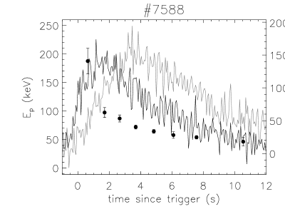
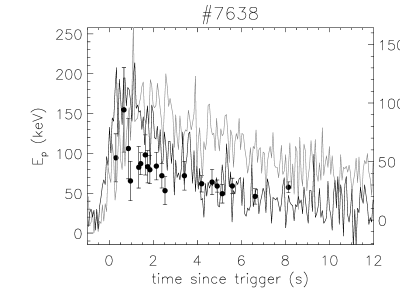
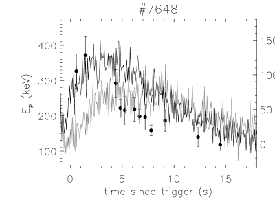
Figure 6: Spectral evolution of $E_{p}$ and temporal behaviors of GRB pulses of BATSE channels 3 and 1 in our sample for the case of hard-to-soft, where the black lines represent the light curves of channel 3. The positive lags are evident.

We first employ the widely used cross-correlation function (CCF) to compute the spectral lags between the pulses of the same burst seen in the BATSE channels 1 and 3. Similar to Norris et al. (2000) we adopt a cubic polynomial to fit the peak of the resulting discrete CCF function and take the peak of the cubic polynomial form as the lag. The error in the average CCF lag, $lag_{13}$, is found by simulations with Gaussian noise added to each of the two channels. These spectral lags resulting from the evolution of hard-to-soft are listed in Table 1. We find no negative lags in the hard-to-soft pulses.

Recently Hakkila et al. (2008) point out that the CCF and pulse peak lags occasionally disagree. In order to further test it we also find pulse peak lags which are defined as the differences between the pulse peak in BATSE channels 1 and 3. In order to find the peak time of pulse we must select a pulse model to fit these pulses. Following Peng et al. (2006) we only select the function presented in equation (22) of Kocevski et al. (2003). We fit those selected background-subtracted pulses using the KRL function. Our fittings are constrained on the channels 1 and 3 to find their difference of peak times. The best fitting parameters are depended on which $\chi_{\nu}^{2}$ of the fitting model is smaller. The pulse peak lags along with the fitting $\chi_{\nu}^{2}$ in channels 1 and 3 are also listed in Table 1. From Table 1 we find all the lags of hard-to-soft pulse are positive. We also check the CCF lags and peak lags by smoothing the light curves with the DB3 wavelet (Qin et al. 2004) and obtain the same results (see, Table 1).

Table 1: A list of various observed lags of GRB pulses whose spectral evolution following from hard to soft

trigger	st (s)	et (s)	$lag_{13,p}$ (s)	$dlag_{13,p}$ (s)	$lag_{13,c}$ (s)	$dlag_{13,c}$ (s)	$\chi_{\nu,1}^{2}$	$\chi_{\nu,3}^{2}$
1406	-2.0	15.0	1.864 $\pm$ 0.169	1.857 $\pm$ 0.169	1.152 $\pm$ 0.019	0.487 $\pm$ 0.509	1.05	1.07
2138	-2.0	15.0	0.988 $\pm$ 0.302	1.001 $\pm$ 0.316	1.024 $\pm$ 0.057	0.604 $\pm$ 0.178	1.10	0.99
2387	-2.0	20.0	2.188 $\pm$ 0.204	2.169 $\pm$ 0.207	1.856 $\pm$ 0.019	1.574 $\pm$ 0.177	1.12	1.15
2662	-2.0	15.0	1.331 $\pm$ 0.285	1.355 $\pm$ 0.272	0.768 $\pm$ 0.159	0.712 $\pm$ 0.139	1.01	1.17
2665	-2.0	15.0	1.552 $\pm$ 0.196	1.555 $\pm$ 0.196	1.507 $\pm$ 0.503	1.417 $\pm$ 0.148	0.89	0.91
3256	-2.0	15.0	2.120 $\pm$ 0.428	2.828 $\pm$ 0.390	1.532 $\pm$ 0.806	1.325 $\pm$ 0.147	1.04	1.07
3257	-1.0	15.0	1.667 $\pm$ 0.517	1.606 $\pm$ 0.509	1.283 $\pm$ 0.075	1.134 $\pm$ 0.094	0.97	0.92
3875	-1.0	5.0	0.262 $\pm$ 0.029	0.257 $\pm$ 0.031	0.162 $\pm$ 0.026	0.169 $\pm$ 0.011	1.40	1.18
4368	-2.0	10.0	0.346 $\pm$ 0.047	0.346 $\pm$ 0.048	0.265 $\pm$ 0.027	0.265 $\pm$ 0.013	1.03	0.82
5621	3.2	4.5	0.032 $\pm$ 0.022	0.076 $\pm$ 0.011	0.028 $\pm$ 0.002	0.030 $\pm$ 0.001	1.24	1.71
6397	-2.0	20.0	1.158 $\pm$ 0.082	1.160 $\pm$ 0.082	0.942 $\pm$ 0.031	0.934 $\pm$ 0.171	1.17	1.70
7548	2.0	12.0	0.814 $\pm$ 0.075	0.816 $\pm$ 0.075	0.596 $\pm$ 0.232	0.628 $\pm$ 0.063	0.88	1.10
7588	-2.0	15.0	2.230 $\pm$ 0.120	2.220 $\pm$ 0.120	1.125 $\pm$ 0.292	1.427 $\pm$ 0.390	0.87	0.93
7638	-2.0	15.0	1.124 $\pm$ 0.114	1.420 $\pm$ 0.134	0.968 $\pm$ 0.012	0.931 $\pm$ 0.162	1.15	1.04
7648	-2.0	15.0	2.490 $\pm$ 0.243	2.501 $\pm$ 0.248	1.574 $\pm$ 1.202	1.528 $\pm$ 0.386	1.01	1.03

Note: st and et denotes the start and end time since bursts trigger of selected pulses, respectively. $lag_{13,p}$ and $lag_{13,c}$ represents peak time lag and CCF lag, while $dlag_{13,p}$ and $dlag_{13,c}$ are the corresponding lags but the light curve having been smoothed with the DB3 wavelet, $\chi_{\nu,1}^{2}$ and $\chi_{\nu,3}^{2}$ is the fitting $\chi_{\nu}^{2}$ of channels 1 and 3, respectively.

6 Conclusions and discussions

Spectral evolution is an established characteristic in GRBs. Moreover the trend for their high-energy photons to arrive before the lower-energy ones (“hard-to-soft” evolution) is universal phenomenon, which leads to positive lags. Kocevski & Liang (2003) showed the robust connection between the spectral lag measured in GRBs and the hard-to-soft evolution of the burst spectra by employing a sample of clean single-peaked bursts with measured lag. In this paper, we have investigated the connection between the evolution of the rest-frame spectral parameters and the spectral lag using a theoretical model derived by Qin (2002) and Qin et al. (2004). We first assume an intrinsic Band spectrum and a Gaussian emission profile to study the issue. Our theoretical analysis shows that the connection exists not only between the hard-to-soft evolution of the burst spectra and the spectral lag but between the soft-to-hard evolution and the spectral lag as well as between the soft-to-hard-to-soft and the spectral lag. In addition, the hard-to-soft spectral parameters evolution can produce the positive lags, while the negative lags may be resulting from the evolution of soft-to-hard as well as soft-to-hard-to-soft. We also take account of the other local pulse forms studied by Qin et al. (2004) and find that the spectral lags resulting from these different local pulses are consistent with those of the Gaussian pulse.

Let us check whether there are any differences in the measurements between peak lags, $Lag_{13}$, adopted in the above analysis and the widely used cross correlation function lags, $CCF_{13}$ (e.g., Norris et al. 2000). Similar to Band (1997) and Norris et al. (2000) we fitted a cubic polynomial to the peak of the resulting discrete CCF function and find the difference of the corresponding peak time. In Fig. 7 the peak lag, $Lag_{13}$, is plotted as a function of the CCF lag, $CCF_{13}$. A linear fit is given which shows that there is a good correspondence between the two methods. The best fit is $Lag_{13}=(-0.03\pm 0.03)+(1.28\pm 0.23)\times CCF_{13}$. The values of intercept and slope are consistent with the results of Ryde et al. (2005). Therefore, the peak lags we used in this study would not affect our analysis results.

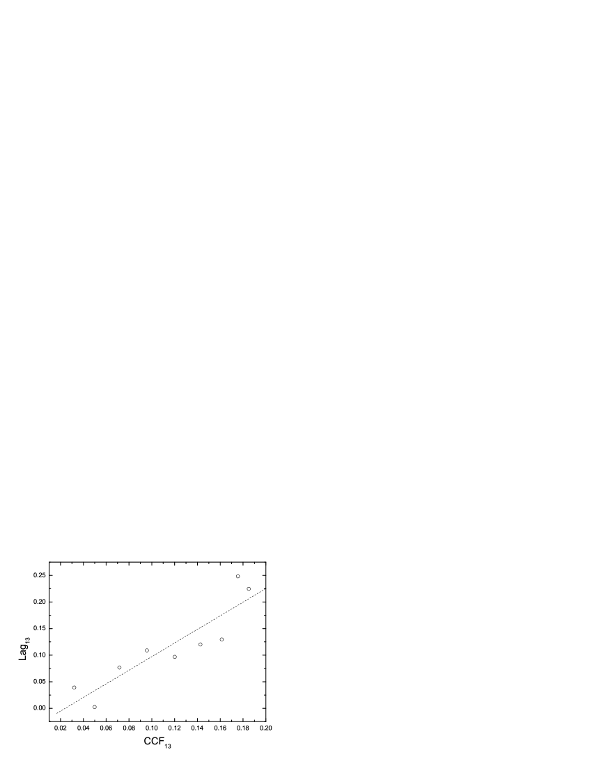
Figure 7: Peak lag (s) versus CCF lag (s). A good linear correspondence exists, as expected.

We select a sample consisting of 15 pulses whose peak energy $E_{p}$ follow hard-to-soft evolution to test our theoretical predictions. Our analysis shows that all of the CCF lags and analytic lags of hard-to-soft pulses are positive within the range of uncertainty. In order to decrease the effect of noise on our results we smoothed the data with the DB3 wavelet (the second-class decomposition) using the MATLAB software (Qin et al. 2004). Then we re-calculate the two types of lags (see, Table 1) and find the lags are also positive. This indicates hard-to-soft spectral evolution may indeed produce positive lags, which is in good agreement with our theoretical prediction.

Currently we can not ascertain if the negative lag predicted by our adopted model are consistent with observation because we are not convinced in the significant existence of negative lags in our observation. The main reasons mentioned in the previous section are the near-zero lags of most pulse as well as the existence of multiple overlapping pulses. Even then we can make a theoretical predication about the producing of the negative lags, i.e. the soft-to-hard and the soft-to-hard-to-soft spectral evolution may give rise to the negative lags, which reserves the further investigations in the future observations.

When taking the spectral evolution and curvature effect into account simultaneously we find the lags are larger than those associated with the case that we only consider the spectral evolution (see, Fig. 5). The two factors must play the roles simultaneously on the producing of the spectral lags since the curvature effect must be play a important role on the producing of spectral and temporal profile of the GRB. In other words, the observed lags should suffer from this two factors simultaneously. Therefore we argue that the number of the observed negative lag should be much smaller than positive lags. Recently, Chen et al. (2005) used the data acquired in the time-to-spill (TTS) mode for long GRBs by BATSE and found that positive lags is the norm in this selected sample set of long GRBs. While relatively few in number, some pulses of several long GRBs do show negative lags, which is also consistent with our theoretical predication.

Both the theory and observation suggest the connection between the spectral evolution and the spectral lags indeed exists. Therefore, we must make clear the mechanism of intrinsic spectral evolution in order to reveal the underlying physics of the spectral lag. To explore this, we must first understand the mechanism that produces breaks in the GRB spectra and what causes its evolution but it is a difficult issue. As for the physical model of hard-to-soft spectral evolution several authors have proposed the possible origin. For example, Tavani (1996) showed the behavior of hard-to-soft spectral evolution are caused by the variation of the average Lorentz factor of pre-accelerated particles and the strength of the local magnetic field at the GRB site as the synchrotron emission evolves within the burst. While Liang (1997) proposed a physical model of hard-to-soft spectral evolution in which impulsively accelerated non-thermal leptons cool by saturated Compton upscattering of soft photons. Kocevski & Liang (2003) pointed out it is a harder question due to uncertainties involved with the microphysics of GRBs. They thought the interpretation of peak energy $E_{p}$ (and hence its evolution) depends on the radiation mechanism that is used to explain the GRB spectra. Moreover they also attempted to examine several mechanisms that could produce the decay of the GRB spectra and discuss how this evolution could be connected to the bursts luminosity for each model. Whereas for the soft-to-hard-to-soft spectral evolution few attempts have been made to explain it. Peng et al. (2009a) argued that the phenomenon may be caused by both kinematic and dynamic process. However they did not provide further evidences to distinguish which one is dominant. The issue of spectral evolution of hard-to-soft and soft-to-hard-to-soft is still unclear, which deserves careful studies and further investigations.

- [1] Band, D. L., Matteson, J., Ford, L., et al.: 1993, ApJ 413, 281
- [2] Band, D. L.: 1997, ApJ 486, 928
- [3] Butler, N. R., Kocevski, D.: 2007, ApJ 663, 407
- [4] Chen, L., Lou, Y. Q., Wu, M., Qu, J. L., Jia, S. M., Yang, X. J.: 2005, ApJ 619, 983
- [5] Cheng, L. X., Ma, Y. Q., Cheng, K. S., Lu, T., Zhou, Y. Y.: 1995, A&A 300, 746
- [6] Crider, A., Liang, E. P., Smith, I. A., et al.: 1997, ApJ 479, L39
- [7] Ford, L. A., Band, D. L., Matteson, J. L., et al.: 1995, ApJ 439, 307
- [8] Hailey, C. J., Harrison, F. A., Mori, K.: 1999, ApJ 520, L25
- [9] Hakkila, J., Giblin, T. W., Norris, J. P., Fragile, P. C., Bonnell, J. T.: 2008, ApJ 677, L81
- [10] Kaneko, Y., Preece, R. D., Briggs, M. S. Paciesas, W. S., Meegan, C. A., Band, D. L.: 2006, ApJS 166, 298
- [11] Kargatis, V. E., Liang, E. P., Hurley, K. C., Barat, C., Eveno, E., Niel, M.: 1994, ApJ 422, 260
- [12] Kocevski, D., Liang, E.: 2003, ApJ 594, 385
- [13] Kocevski, D., Ryde, F., Liang, E.: 2003, ApJ 596, 389
- [14] Liang, E.: 1997, ApJ 491, L15
- [15] Lu, R. J., Qin, Y. P., Zhang, Z. B., Yi, T. F.: 2006, MNRAS 367, 275
- [16] Mészáros, P., Rees, M. J.: 1998, ApJ 502, L105
- [17] Norris, J. P., Marani, G. F., Bonnell, J. T.: 2000, ApJ 534, 248
- [18] Norris, J. P., Bonnell, J. T., Kazanas, D., Scargle, J. D., Hakkila, J., Giblin, T. W.: 2005, ApJ 627, 324
- [19] Peng, Z. Y., Qin, Y. P., Zhang, B. B., Lu, R. J., Jia, L. W., Zhang, Z.B.: 2006, MNRAS 368, 1351
- [20] Peng, Z. Y., Lu, R. J., Zhang, B. B., Qin, Y. P.: 2007, ChjAA 7, 428
- [21] Peng, Z. Y., Ma, L. Lu, R. J. Fang, L.M. Bao, Y. Y., Yin, Y.: 2009a, NewA 14, 311
- [22] Peng, Z. Y., Ma, L., Zhao, X. H., Yin, Y. Fang, L. M. Bao, Y. Y.: 2009b, ApJ 698, 417
- [23] Peng, Z. Y., Yin, Y., Bi, X. W., Zhao, X. H., Fang, L. M., Bao, Y. Y., Ma, L.: 2010, ApJ 718, 894
- [24] Preece, R. D., Briggs, M. S., Mallozzi, R. S., Pendleton, G. N., Paciesas, W. S., Band, D. L.: 1998, ApJ 496, 849
- [25] Preece, R. D., Briggs, M. S., Mallozzi, R. S., Pendleton, G. N., Paciesas, W. S., Band, D. L.: 2000, ApJS 126, 19
- [26] Qin, Y. P.: 2002, A&A 396, 705
- [27] Qin, Y. P., Zhang, Z. B., Zhang, F. W., Cui X. H.: 2004, ApJ 617, 439
- [28] Qin, Y. P., Dong, Y. M., Lu, R. J., Zhang, B. B., Jia, L. W.: 2005, ApJ 632,1008
- [29] Qin, Y. P., Su, C. Y., Fan, J. H., Gupta A. C.: 2006, Phys. Rev. D 74, 063005
- [30] Qin, Y. P. 2008, ApJ, 683, 900
- [31] Qin, Y. P., Gupta, A. C., Fan, J. H., Lu, R.-J.: 2008, JCAP 11, 004
- [32] Qin, Y. P.: 2009, ApJ 691, 811
- [33] Ryde, F., Petrosian, V.: 2002, ApJ 578, 290
- [34] Ryde, F., Kocevski, D., Bagoly, Z., Ryde, N., Mészáros, A.: 2005, A&A 432, 105
- [35] Schaefer, B. E.: 2004, ApJ 602, 306
- [36] Shen, R. F., Song, L. M., Li, Z.: 2005, MNRAS 362, 59
- [37] Tavani, M.: 1996, ApJ 466, 768
- [38] Wu, B., Fenimore, E.: 2000, ApJ 535, L29
- [39] Yi, T. F., Liang, E. W., Qin, Y. P., Lu, R. J.: 2006, MNRAS 367, 1751