Linear-Space Data Structures for Range Mode Query in Arrays

Abstract

A mode of a multiset $S$ is an element $a\in S$ of maximum multiplicity; that is, $a$ occurs at least as frequently as any other element in $S$. Given a list $A[1:n]$ of $n$ items, we consider the problem of constructing a data structure that efficiently answers range mode queries on $A$. Each query consists of an input pair of indices $(i,j)$ for which a mode of $A[i:j]$ must be returned. We present an $O(n^{2-2\epsilon})$-space static data structure that supports range mode queries in $O(n^{\epsilon})$ time in the worst case, for any fixed $\epsilon\in[0,1/2]$. When $\epsilon=1/2$, this corresponds to the first linear-space data structure to guarantee $O(\sqrt{n})$ query time. We then describe three additional linear-space data structures that provide $O(k)$, $O(m)$, and $O(|j-i|)$ query time, respectively, where $k$ denotes the number of distinct elements in $A$ and $m$ denotes the frequency of the mode of $A$. Finally, we examine generalizing our data structures to higher dimensions.

1 Introduction

Mode and Range Queries. The frequency of an element $x$ in a multiset $S$, denoted $\operatorname{freq}_{S}(x)$, is the number of occurrences (i.e., the multiplicity) of $x$ in $S$. A mode of $S$ is an element $a\in S$ such that for all $x\in S$, $\operatorname{freq}_{S}(x)\leq\operatorname{freq}_{S}(a)$. A multiset $S$ may have multiple distinct modes; the frequency of the modes of $S$, denoted by $m$, is unique.

Along with the mean and median of a multiset, the mode is a fundamental statistic of data analysis for which efficient computation is necessary. Given a sequence of $n$ elements ordered in a list $A$, a range query seeks to compute the corresponding statistic on the multiset determined by a subinterval of the list: $A[i:j]$. The objective is to preprocess $A$ to construct a data structure that supports efficient response to one or more subsequent range queries, where the corresponding input parameters $(i,j)$ are provided at query time.

We assume the RAM model of computation with word size $\Theta(\log u)$, where elements are drawn from a universe $U=\{0,\ldots,u-1\}$. Although the complete set of possible queries can be precomputed and stored using $\Theta(n^{2})$ space, practical data structures require less storage while still enabling efficient response time. For all $i$, if $i=j$, then a range query must report $A[i]$. Consequently, any range query data structure for a list of $n$ items requires $\Omega(n)$ storage space in the worst case [7]. This leads to a natural question: how quickly can an $O(n)$-space data structure answer range queries? The problem of constructing efficient data structures for range median queries has been analyzed extensively [7, 9, 10, 11, 23, 24, 26, 28, 29, 30, 33, 34]. A range mean query is equivalent to a normalized range sum query (partial sum query), for which a precomputed prefix-sum array provides a linear-space static data structure with constant query time [30]. As expressed recently by Brodal et al. regarding the current status of the range mode query problem: “The problem of finding the most frequent element within a given array range is still rather open.” [9, page 2]. See Section 1 for an overview of the current state of the range mode query problem.

Our Results. Given an array $A[1:n]$ of $n$ items, we present an $O(n^{2-2\epsilon})$-space static data structure that supports range mode queries in $O(n^{\epsilon})$ time in the worst case, for any fixed $\epsilon\in[0,1/2]$. When $\epsilon=1/2$, this corresponds to the first linear-space data structure to guarantee $O(\sqrt{n})$ query time. Prior to our work, the previous fastest linear-space data structure by Krizanc et al. [30] supported range mode queries in $O(\sqrt{n}\log\log n)$ time; our data structure borrows ideas developed by Krizanc et al. and augments their data structure to eliminate dependence on predecessor queries (see Proposition 4). We describe three additional $O(n)$-space data structures that provide $O(k)$, $O(m)$, and $O(|j-i|)$ query time, respectively, where $k$ denotes the number of distinct elements in $A$. Finally we discuss generalizations of our data structures to $d$ dimensions for any fixed $d$. To the authors’ knowledge, this is the first examination of multidimensional range mode query.

2 Related Work

Computing a Mode. The mode of a multiset $S$ of $n$ items can be found in $O(n\log n)$ time by sorting $S$ and scanning the sorted list to identify the longest sequence of identical items. Due to the corresponding lower bound on the worst-case time for solving the element uniqueness problem, finding a mode requires $\Omega(n\log n)$ time in the worst case; that is, the decision problem of determining whether $m>1$ requires $\Omega(n\log n)$ time in the worst case [36]. Better bounds on the worst-case time are obtained by parameterizing in terms of $m$ or $k$. A worst-case time of $O(n\log k)$ is easily achieved by inserting the $n$ elements into a balanced search tree in which each node stores a key and its frequency. Munro and Spira [32] describe an $O(n\log(n/m))$-time algorithm for finding a mode and a corresponding lower bound of $\Omega(n\log(n/m))$ on the worst-case time.

If distinct elements in $S$ can be mapped efficiently (i.e., in constant time) to distinct integers in the range $\{1,\ldots,k^{\prime}\}$, for some $k^{\prime}$, then a mode of $S$ can be found in $O(n+k^{\prime})$ time using $O(n+k^{\prime})$ space. This is achieved by identifying a maximum element in a frequency table for $S$ of size $k^{\prime}$. This method is analogous to counting sort. A similar algorithm for computing a mode can be implemented using hash tables.

We include the following lemma to which we refer in Section 3:

Lemma 1 (Krizanc et al. [30])

Let $A$ and $B$ be any multisets. If $c$ is a mode of $A\cup B$ and $c\not\in A$, then $c$ is a mode of $B$.

Range Mode Query. Naturally, a mode of the query interval $A[i:j]$ can be computed directly without preprocessing using any of the methods described in Section 2. Krizanc et al. [30] describe data structures that provide constant-time queries using $O(n^{2}\log\log n/\log n)$ space and $O(n^{\epsilon}\log n)$-time queries using $O(n^{2-2\epsilon})$ space, for any fixed $\epsilon\in(0,1/2]$. Petersen and Grabowski [34] improve the first bound to constant time and $O(n^{2}\log\log n/\log^{2}n)$ space and Petersen [33] improves the second bound to $O(n^{\epsilon})$-time queries using $O(n^{2-2\epsilon})$ space, for any fixed $\epsilon\in[0,1/2)$. When $\epsilon=1/2$, the data structure of Krizanc et al. [30] requires only linear space and provides $O(\sqrt{n}\log\log n)$ query time. Although its space requirement is almost linear in $n$ as $\epsilon$ approaches $1/2$, the data structure of Petersen [33] requires $\omega(n)$ space. Furthermore, the construction becomes impractical as $\epsilon$ approaches $1/2$ (the number of levels in a hierarchical set of tables and hash functions approaches $\infty$ as $\epsilon\to 1/2$) and no obvious modification reduces its space requirement to $O(n)$. Greve et al. [25] prove a lower bound of $\Omega(\log n/\log(s\cdot w/n))$ query time for any data structure that uses $s$ memory cells of $w$ bits.

Bose et al. [7] consider approximate range mode queries, in which the objective is to return an element whose frequency is at least $\alpha\cdot m$. They give a data structure that requires $O(n/(1-\alpha))$ space and answers approximate range mode queries in $O(\log\log_{1/\alpha}n)$ time for any fixed $\alpha\in(0,1)$, as well as data structures that provide constant-time queries for $\alpha\in\{1/2,1/3,1/4\}$, using space $O(n\log n)$, $O(n\log\log n)$, and $O(n)$, respectively. Greve et al. [25] give a linear-space data structure that supports approximate range mode queries in constant time for $\alpha=1/3$, and an $O(n\cdot\alpha/(1-\alpha))$-space data structure that supports approximate range mode queries in $O(\log(\alpha/(1-\alpha)))$ time for any fixed $\alpha\in[1/2,1)$.

Continuous Space versus Array Input. A vast literature studies the problems of geometric range searching in continuous Euclidean space; that is, data points are positioned arbitrarily in $\mathbb{R}^{d}$. See the survey by Agarwal [1] for an overview of results. The range query problems considered in this paper, however, restrict attention to array input. Although a range query on an array can be viewed as a restricted case of a more general range searching problem (e.g., a point set with regular spacing), the algorithmic techniques differ greatly between the two settings when $d\geq 2$. When $d=1$, however, a geometric range mode query problem reduces to array range mode query. In particular, the rank of each data point in Euclidean space corresponds to its array index. It suffices to compute the ranks of the respective successor and predecessor of the endpoints of the query interval to identify the indices $i$ and $j$, and to return the corresponding array range mode query on $A[i:j]$.

In addition to results on the median, mode, and sum range query problems discussed in Sections 1 and 1, other range query problems examined on arrays include semigroups [2, 38, 39], extrema (e.g., range minimum or maximum) [4, 6, 13, 19, 20, 18, 21, 22], selection or quantiles (for which the median is a special case) [23, 24, 28, 29], dominance or rank (counting the number of elements in the query range that exceed a given input threshold) [27, 28], coloured range (counting/enumerating the distinct elements in the query range) [23], and $k$-frequency (determining whether any element has frequency $k$) [25]. Recently, range query problems have been examined on multidimensional arrays, including partial sums [12], range minimum [3, 8, 13, 35, 40], median [24], and selection [23].

3 Sparse Mode Table Method: $O(n^{\epsilon})$ Query Time and $O(n^{2-2\epsilon})$ Space

In the worst case, for every range mode query processed, the data structure of Krizanc et al. [30] makes a sequence of $\Theta(n^{\epsilon})$ predecessor queries, each requiring $\Theta(\log\log n)$ time, for a total query time of $\Theta(n^{\epsilon}\log\log n)$. We build on the data structure of Krizanc et al. and introduce a different technique that avoids predecessor search entirely. Section 3 establishes the following theorem and the corresponding corollary that follows when $\epsilon=1/2$:

Theorem 2

Given an array $A[1:n]$ of $n$ items, for any $\epsilon\in[0,1/2]$ there exists a data structure requiring $O(n^{2-2\epsilon})$ storage space that supports range mode queries on $A$ in $O(n^{\epsilon})$ time in the worst case.

Corollary 3

Given an array $A[1:n]$ of $n$ items, there exists a data structure requiring $O(n)$ storage space that supports range mode queries on $A$ in $O(\sqrt{n})$ time in the worst case.

Data Structure Precomputation. Suppose the elements of $A[1:n]$ are drawn from an ordered bounded universe $U$. Let $D=\{a_{1},\ldots,a_{k}\}\subseteq U$ denote the set of distinct elements stored in $A$. Construct an array $B[1:n]$ such that for each $i$, $B[i]$ stores the rank of $A[i]$ in $D$. Therefore, $B[i]\in\{1,\ldots,k\}$. For any $a$, $i$, and $j$, $B[a]$ is a mode of $B[i:j]$ if and only if $A[a]$ is a mode of $A[i:j]$. Performing computation on array $B$ instead of array $A$ allows direct array referencing using the values stored in $B$ as indices. For simplicity, we describe our data structures in terms of array $B$; a table look-up provides a direct bijective mapping from $\{1,\ldots,k\}$ to $D$. Set $D$, array $B$, and the value $k$ are independent of any query range and can be computed in $O(n\log k)$ time during preprocessing.

Given fixed $a$ and $b$, array $C[1:k]$ is a frequency table for $B[a:b]$ if, for each $i$, $C[i]$ stores the number of occurrences of element $i$ in $B[a:b]$. For any $j>i$, if $C_{i}[1:k]$ is a frequency table for $B[1:i]$ and $C_{j}[1:k]$ is a frequency table for $B[1:j]$, then for each $x$, $C_{j}[x]-C_{i}[x]$ is the frequency of $B[x]$ in $B[i+1:j]$.

For each $a\in\{1,\ldots,k\}$, let $Q_{a}=\{b\mid B[b]=a\}$. That is, $Q_{a}$ is the set of indices $b$ such that $B[b]=a$. For any $a$, a range counting query for element $a$ in $B[i:j]$ can be answered by searching for the predecessors of $i$ and $j$, respectively, in the set $Q_{a}$; the difference of the indices of the two predecessors is the frequency of $a$ in $B[i:j]$ [30]. As noted above, implementing such a range counting query using an efficient predecessor data structure requires $\Theta(\log\log n)$ time in the worst case.

The following related decision problem, however, can be answered in constant time by a linear-space data structure: does $B[i:j]$ contain at least $q$ instances of element $B[i]$? This question can be answered by a select query that returns the index of the $q$th instance of $B[i]$ in $B[i:n]$. For each $a\in\{1,\ldots,k\}$, store the set $Q_{a}$ as an ordered array (also denoted $Q_{a}$ for simplicity). Define a rank array $B^{\prime}[1:n]$ such that for all $b$, $B^{\prime}[b]$ denotes the rank of $B[b]$ in $B[1:n]$ (i.e., the index of $b$ in $Q_{B[b]}$). Given any $q$, $i$, and $j$, to determine whether $B[i:j]$ contains at least $q$ instances of $B[i]$ it suffices to check whether $Q_{B[i]}[B^{\prime}[i]+q-1]\leq j$. Since array $Q_{B[i]}$ stores the sequence of indices of instances of element $B[i]$ in $B$, looking ahead $q-1$ positions in $Q_{B[i]}$ returns the index of the $q$th occurrence of element $B[i]$ in $B[i:n]$; if this index is at most $j$, then the frequency of $B[i]$ in $B[i:j]$ is at least $q$. If the index $B^{\prime}[i]+q-1$ exceeds the size of the array $Q_{B[i]}$, then the query returns a negative answer. This gives the following lemma:

Lemma 4

Given an array $A[1:n]$ of $n$ items, there exists a data structure requiring $O(n)$ storage space that can determine in constant time for any $\{i,j\}\subseteq\{1,\ldots,n\}$ and any $q$ whether $A[i:j]$ contains at least $q$ instances of element $A[i]$.

Following Krizanc et al. [30], given any $\epsilon\in[0,1/2]$ we partition array $B$ into $t$ blocks of size $s=\lceil n^{\epsilon}\rceil$, where $t=\lceil n/s\rceil\leq\lceil n^{1-\epsilon}\rceil$. That is, for each $i\in\{0,\ldots,t-2\}$, the $i$th block spans $B[i\cdot s+1:(i+1)s]$ and the last block spans $B[(t-1)\cdot s+1:n]$. We precompute tables $S[0:t-1,0:t-1]$ and $S^{\prime}[0:t-1,0:t-1]$, each of size $\Theta(t^{2})$, such that for any $\{b_{i},b_{j}\}\subseteq\{0,\ldots,t-1\}$, $S[b_{i},b_{j}]$ stores a mode of $B[b_{i}\cdot s+1:(b_{j}+1)s]$ and $S^{\prime}[b_{i},b_{j}]$ stores the corresponding frequency.

Finally, we need a frequency table $C[1:k]$ of size $k$, initialized to zero. The arrays $Q_{1},\ldots,Q_{k}$ can be constructed in $O(n)$ total time in a single scan of array $B$. The arrays $S$ and $S^{\prime}$ can be constructed in $O(n^{2-\epsilon})$ time by scanning array $B$ $t$ times, computing one row of each array $S$ and $S^{\prime}$ per scan. Thus, the total precomputation time required to initialize the data structure is $O(n^{2-\epsilon})$.

Range Mode Query Algorithm. Given a query range $B[i:j]$, let $b_{i}=\lceil(i-1)/s\rceil$ and $b_{j}=\lfloor j/s\rfloor-1$ denote the respective indices of the first and last blocks completely contained within $B[i:j]$. We refer to $B[b_{i}\cdot s+1:(b_{j}+1)s]$ as the span of the query range, to $B[i:\min\{b_{i}\cdot s,j\}]$ as its prefix, and to $B[\max\{(b_{j}+1)s+1,i\}:j]$ as its suffix. One or more of the prefix, span, and suffix may be empty; in particular, if $b_{i}>b_{j}$, then the span is empty. See the example in Figure 1.

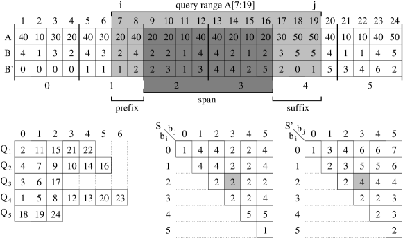
Figure 1: Example of the sparse mode table method data structure. The number of list items is $n=24$, of which $k=5$ are distinct. If $\epsilon=3/8$, the array is partitioned into $t=\lceil n/s\rceil=6$ blocks of size $s=\lceil n^{\epsilon}\rceil=4$. The query range is $A[i:j]=A[7:19]$, for which the unique mode is 20, occurring with frequency 5. The corresponding mode of $B[i:j]$ is 2. The query range $B[7:19]$ is partitioned into the prefix $B[7:8]$, the span $B[9:16]$, and the suffix $B[17:19]$. The span covers blocks $b_{i}=2$ to $b_{j}=3$, for which the corresponding mode is $S[2,3]=2$, occurring with frequency $S^{\prime}[2,3]=4$.

The value $c=S[b_{i},b_{j}]$ is a mode of the span with corresponding frequency $f_{c}=S^{\prime}[b_{i},b_{j}]$. If the span is empty, then let $f_{c}=0$. By Lemma 1, either $c$ is a mode of $B[i:j]$ or some element of the prefix or suffix is a mode of $B[i:j]$. Thus, to identify a mode of $B[i:j]$, we verify for every element in the prefix and suffix whether its frequency in $B[i:j]$ exceeds $f_{c}$ and, if so, we identify this element as a candidate mode and count its additional occurrences in $B[i:j]$. We present the details of this procedure for the prefix; an analogous procedure is applied to the suffix.

We now describe how to compute the frequency of all candidate elements in the prefix over the range $B[i:j]$, storing these values in the frequency table $C$. Sequentially scan the items in the prefix starting at the leftmost index, $i$, and let $x$ denote the index of current item. If $C[B[x]]>0$, then an instance of element $B[x]$ appears in $B[i:x-1]$, and its frequency has been counted already; in this case, simply skip $B[x]$ and increment $x$. If $C[B[x]]=0$, check whether $Q_{B[x]}[B^{\prime}[x]+f_{c}-1]\leq j$ (i.e., verify whether $B[x]$ is a candidate). If so, then the frequency of $B[x]$ in $B[i:j]$ is at least $f_{c}$. The exact frequency of $B[x]$ in $B[i:j]$ can be counted by a linear scan of $Q_{B[x]}$, starting at index $B^{\prime}[x]+f_{c}-1$ and terminating upon reaching either an index $y$ such that $Q_{B[x]}[y]>j$ or the end of array $Q_{B[x]}$ (i.e., $y=|Q_{B[x]}|+1$). That is, $Q_{B[x]}[y]$ denotes the index of the first instance of element $B[x]$ that lies beyond the query range $B[i:j]$ (or no such element exists). Consequently, the frequency of $B[x]$ in $B[i:j]$ is $y-B^{\prime}[x]$. Store this value in $C[B[x]]$.

An analogous procedure is repeated for the suffix. Upon completing the scans of the prefix and suffix, we identify a maximum value in array $C$; its index corresponds to a mode of $B[i:j]$. Only non-zero entries in $C$ need be examined (and subsequently reset to zero); this is achieved by making a second scan of the prefix and suffix and examining the corresponding elements in array $C$.

Storage Space and Query Time. If the prefix and suffix are empty, then $S[b_{i},b_{j}]$ is a mode of $B[i:j]$, and this value is returned in constant time. Without loss of generality, suppose the prefix contains at least one item. Consider an arbitrary index $x\in\{i,\ldots,b_{i}\cdot s-1\}$ during the scan of the prefix. If $C[B[x]]>0$, then $B[x]$ is processed in constant time. Therefore, suppose $C[B[x]]=0$. That is, $x$ corresponds to the index of the first instance of $B[x]$ in the prefix. Consequently, the frequency of $B[x]$ in $B[i:j]$, denoted $f_{x}$, is equal to its frequency in $B[x:j]$. By Lemma 4, determining whether $f_{x}\geq f_{c}$ requires only constant time. Any item $B[x]$ that is not a candidate is processed in constant time. Therefore, suppose $B[x]$ is a candidate. Since the prefix and suffix each have size at most $s-1$, $f_{c}\leq f_{x}\leq 2(s-1)$.

Item $B[x]$ incurs a cost of $O(f_{x}-f_{c})$ time for its first occurrence, and $O(1)$ time for subsequent occurrences. Since $f_{c}$ is the frequency of the mode of the span, at least $f_{x}-f_{c}$ instances of $B[x]$ must occur in the prefix or suffix. In other words, instances of element $B[x]$ incur a total cost of $O(c_{x})$ time, where $c_{x}$ denotes the frequency of $B[x]$ in the prefix and suffix. Since the number of items in the prefix and suffix is at most $2(s-1)$, the total cost for processing the prefix is $O(s)$. By an analogous argument, the total cost for processing the suffix is also $O(s)$. Identifying the maximum element in array $C$ and re-initializing $C$ to zero requires $O(s)$ time. Therefore, a range mode query requires $O(s)=O(n^{\epsilon})$ time in the worst case. The data structure requires $O(n)$ space to store the arrays $A$, $B$, and $B^{\prime}$, $O(n)$ total space to store the arrays $Q_{1},\ldots,Q_{k}$, and $O(t^{2})=O(n^{2-2\epsilon})$ space to store the tables $S$ and $S^{\prime}$. This gives $O(n^{2-2\epsilon})$ total space for $O(n^{\epsilon})$ worst-case query time for any $\epsilon\in[0,1/2]$, proving Theorem 2. As mentioned earlier, $\Omega(n)$ space is required. Therefore, increasing $\epsilon$ beyond $1/2$ increases query time without decreasing space.

4 Additional Linear-Space Range Mode Query Data Structures

We apply results from Section 3 to obtain three additional $O(n)$-space data structures, giving the following theorem:

Theorem 5

Given an array $A[1:n]$ of $n$ items, there exists a data structure requiring $O(n)$ storage space that supports range mode queries on any $A[i:j]$ in $O(\min\{\sqrt{n},k,|j-i|,m+\log\log n\})$ time in the worst case, where $k$ denotes the number of distinct elements in $A$ and $m$ denotes the frequency of the mode of $A$.

4.1 Sparse Frequency Table Method: $O(k)$ Query Time and $O(n)$ Space

We now describe an $O(k+s)$ query time and $O(n+n\cdot k/s)$-space data structure for any fixed $s\in[1,n]$. When $s\in\Theta(k)$, our data structure requires $O(n)$ space and supports range mode queries in $O(k)$ time. A value of $s\in o(k)$ (respectively, $s\in\omega(k)$) results in $\omega(n)$ space ($\omega(k)$ time) without any reduction in query time (space).

Data Structure Precomputation. For each $p\in\{1,\ldots,n\}$ such that $p\bmod s=0$, construct a frequency table $C_{p}[1:k]$ for the range $B[1:p]$. Create one additional array $C_{0}[1:k]$, initialized to zero. There are $\lceil n/s\rceil+1$ such arrays $C_{i}$. See Figure 2. The preprocessing time required is $O(n+n\cdot k/s)$ (or $O(n\log k+n\cdot k/s)$ time if $k$ or $B$ must be computed).

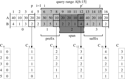
Figure 2: Example of the sparse frequency table method data structure. The number of list items is $n=16$, of which $k=5$ are distinct. The array is partitioned into four blocks of size $s=4$. The query range is $A[i:j]=A[6:15]$, for which elements 10 and 20 are modes, each occurring with frequency 3. The corresponding modes of $B[i:j]$ are 1 and 2. Thus, $C[1]=C[2]=3$ is the maximum value in the frequency array $C$.

Range Mode Query Algorithm. Array $B$ is partitioned into blocks of size $s$ as in Section 3. Given a query range $B[i:j]$, we refer to the sequence of blocks completely covered by $B[i:j]$ as the span, and to the remaining subarrays as the prefix and suffix, respectively. A query on $B[i:j]$ is performed as follows:

1. Let $p=s\lfloor(i-1)/s\rfloor$ and let $p^{\prime}=s\lfloor j/s\rfloor$. That is, $p$ is the largest $p\leq i-1$ such that array $C_{p}$ is defined. Similarly, $p^{\prime}$ is the largest $p^{\prime}\leq j$ such that array $C_{p^{\prime}}$ is defined.

2. Create an array $C[1:k]$ such that for each $x$, $C[x]\leftarrow C_{p^{\prime}}[x]-C_{p}[x]$. Upon completing this step, $C$ is a frequency table for the span $B[p+1:p^{\prime}]$.

3. For each $x\in\{p+1,\ldots,i-1\}$, set $C[B[x]]\leftarrow C[B[x]]-1$. For each $x\in\{p^{\prime}+1,\ldots,j\}$, set $C[B[x]]\leftarrow C[B[x]]+1$. Upon completing this step $C$ is a frequency table for the entire query range $B[i:j]$.

4. Find a maximum value in $C$. If $x^{\prime}$ is an index that maximizes $C[x^{\prime}]$, then $B[x^{\prime}]$ is a mode of $B[i:j]$.

Storage Space and Query Time. The data structure consists of arrays $A$ and $B$, requiring $O(n)$ space, and $O\lceil n/s\rceil+1$ frequency tables of size $k$. Thus, the total space required by the data structure is $O(n+n\cdot k/s)$. Steps 1 through 4 of the algorithm require $O(1)$, $O(k)$, $O(s)$, and $O(k)$ time, respectively. This gives $O(n+n\cdot k/s)$ total space for $O(k+s)$ query time.

4.2 Low Frequency Mode Method: $O(m+\log\log n)$ Query Time and $O(n)$ Space

Using a combination of ideas from Section 3 and from an approximate range mode query data structure of Greve et al. [25], we briefly describe a range mode data structure parameterized in terms of the frequency of the mode, $m$, with good bounds on space and query time when $m$ is small (e.g., $m\in O(\sqrt{n})$).

As in Section 3, the rank array $B^{\prime}$ and the arrays $Q_{1},\ldots,Q_{k}$ are constructed, and array $B$ is partitioned into blocks of size $s$. For each $i\in\{0,\ldots,n\}$ such that $i\bmod s=0$, construct an array $F_{i}[1:m]$ such that for each $x$, $F_{i}[x]$ stores the largest $j\leq n$ such that the mode of $B[i:j]$ has frequency at most $x$; a corresponding mode is also stored. A query range $B[i:j]$ is divided into prefix, span, and suffix subarrays as before. Let $p=s\lceil i/s\rceil$ denote the index of the first element of the span. Using the technique of Greve et al. [25], a mode of the span and its frequency are computed by finding the successor of $j$ in $F_{i}$; this can be achieved in $O(\log\log n)$ time by an $O(n)$-space data structure (e.g., a van Emde Boas tree [15, 17, 16] or a y-fast trie [37]). By Lemma 4, determining whether the frequency of an element in the prefix or suffix exceeds that of the mode of the span requires only constant time per element, or $O(s)$ total time. The resulting worst-case query time is $O(s+\log\log n)$ using $O(n+n\cdot m/s)$ space. Choosing $s\in\Theta(m)$ gives $O(n)$ space and $O(m+\log\log n)$ query time.

4.3 Counting Method: $O(|j-i|)$ Query Time and $O(n)$ Space

We briefly describe an $O(|j-i|)$-time and $O(n)$-space data structure. No actual precomputation is necessary other than constructing the array $B$, finding $k$, and initializing a frequency table $C[1:k]$ to zero, all of which can be achieved in $O(n\log k)$ precomputation time. This algorithm is similar to counting sort: compute a frequency table for $B[i:j]$ stored in $C[1:k]$, then identify a maximum element in $C[1:k]$. When computing the maximum, the running time is bounded to $O(|j-i|)$ by only examining indices in $C$ that correspond to elements in $B[i:j]$ (these are exactly the elements of $C$ that have non-zero values). This procedure is repeated after identifying the maximum to reset $C[1:k]$ to zero. Each step requires $\Theta(|j-i|)$ time and the total space required by the data structure is $O(n)$.

5 Higher Dimensions

A natural question is whether our results for one-dimensional range mode query extend to arbitrary dimensions. The array $B[1:n]$ is replaced by a $d$-dimensional array $B[1:n_{1},\ldots,1:n_{d}]$, containing $n$ elements in total with dimensionality $n_{1},\ldots,n_{d}$, where $n=n_{1}\times\cdots\times n_{d}$. Within Section 5 we refer to a $d$-dimensional tuple (e.g., $\vec{i}=[i_{1},\ldots,i_{d}])$ as an array index (e.g., $B[\vec{i}]$). We say a tuple $\vec{i}$ dominates another tuple $\vec{j}$ if and only if $i_{t}\leq j_{t}$ for all $t\in\{1,\ldots,d\}$. We denote the input array as $B[\vec{1}:\vec{n}]$, where $\vec{n}=[n_{1},\ldots,n_{d}]$. A range is defined over a $d$-dimensional rectangle of indices, uniquely determined by two indices, $[\vec{i}:\vec{j}]$, where $\vec{i}\leq\vec{j}$.

A key element of our one-dimensional data structures is the use of frequency tables. In $d$ dimensions, array $C[1:k]$ is a frequency table for $B[\vec{a}:\vec{b}]$ if, for each $i\in\{1,\ldots,k\}$, $C[i]$ stores the number of occurrences of element $B[\vec{x}]=i$ in $B[\vec{a}:\vec{b}]$. Unlike the one-dimensional case, if $C_{\vec{i}}[1:k]$ is a frequency table for $B[\vec{1}:\vec{i}]$ and $C_{\vec{j}}[1:k]$ is a frequency table for $B[\vec{1}:\vec{j}]$, then $C_{\vec{j}}[B[\vec{x}]]-C_{\vec{i}}[B[\vec{x}]]$ is not the frequency of $B[\vec{x}]$ in $B[\vec{i}:\vec{j}]$ in general. In one dimension, $\vec{i}$ dominates all indices that are to be excluded from the count, whereas this is not the case in higher dimensions. Instead, the $2^{d}$ corners of the $d$-rectangle $[\vec{i}:\vec{j}]$ can be used to compute the frequency table with typical inclusion-exclusion rules [14]. The result is computed using $2^{d}$ $d$-directional range counting queries to determine the frequency of $B[\vec{x}]$ in $B[\vec{a}:\vec{b}]$. In the range searching literature it is typical to assume $d$ to be a small known constant and for the corresponding factors of $d$ to be omitted from the evaluation of space and time requirements.

Counting Method. The counting method described in Section 4.3 does not depend on any properties of one-dimensional data and extends to $d$-dimensional data and queries. The query time is directly proportional to the cardinality of the query range $[\vec{i}:\vec{j}]$: $O(\prod_{l=1}^{d}(j_{l}-i_{l}+1))$. Precomputation time, query time, and space requirements are analogous to those of the one-dimensional data structure.

Sparse Frequency Table Method. We now consider a generalization to $d$ dimensions of the sparse frequency table method described in Section 4.1. As in the one-dimensional data structure, for every $\vec{t}\in T$ we precompute a frequency table $C_{\vec{t}}[1:k]$ for the range $B[\vec{1}:\vec{t}]$, where $T\subseteq[\vec{1}:\vec{n}]$ is a fixed subset of indices. If $T$ is a sparse set whose elements are distributed regularly across $[\vec{1},\vec{n}]$, then a frequency table for the span can be computed in $O(2^{d}k)$ time and $O(n)$ space using the inclusion-exclusion principle. The remainder of the query algorithm consists of examining each index $\vec{w}$ in the enclosing set $W=[\vec{i}:\vec{j}]\setminus[\vec{b_{i}}:\vec{b_{j}}]$ (known as the suffix and prefix in the one-dimensional case) and incrementing the corresponding frequency count $C[B[\vec{w}]]$. Finally, the maximum value of the frequency table $C$ determines the frequency of the mode; this maximum is identified in $O(k)$ time. Therefore, the total query time is $O(2^{d}k+|W|)$.

The regular positioning of the indices in $T$ forms a $d$-dimensional grid that divides $B[\vec{1}:\vec{n}]$ evenly into $|T|$ cells, each of which is a $d$-rectangle of cardinality $s=n/|T|$. Each frequency table has size $k$. In order for the space occupied by the frequency tables to remain linear there can be at most $O(n/k)$ such tables (e.g., let $|T|=\lceil n/k\rceil$ and $s=k$). We set the width of each cell in the $l$ dimension to be $O(n_{l}(k/n)^{\frac{1}{d}})$. Observe that $\prod_{l=1}^{d}n_{l}(k/n)^{\frac{1}{d}}=k$. Since there are $s=k$ items in a cell, the number of items on the cell’s surface perpendicular to dimension $l$ is

$$O\left(\frac{k}{n_{l}}\left(\frac{n}{k}\right)^{\frac{1}{d}}\right)=O\left(k^{\frac{d-1}{d}}\frac{n^{\frac{1}{d}}}{n_{l}}\right).$$

Observe that $|W|$ is at most $s$ times the number of cells on the external surfaces of the $d$-rectangle specified by the query range $[\vec{i},\vec{j}]$. The total number of items on the external surface perpendicular to some dimension $l\in\{1,\ldots,d\}$ is $O(n/n_{l})$. Thus the number of cells on that external surface is

$$O\left(\frac{n}{n_{l}}\frac{1}{k^{\frac{d-1}{d}}}\frac{n_{l}}{n^{\frac{1}{d}}}\right)=O\left(\left(\frac{n}{k}\right)^{\frac{d-1}{d}}\right).$$

Therefore, $|W|\in O(d\cdot k(n/k)^{\frac{d-1}{d}})=O(d\cdot n^{\frac{d-1}{d}}k^{\frac{1}{d}})$, resulting in a total query time of $O(2^{d}k+d\cdot n^{\frac{d-1}{d}}k^{\frac{1}{d}})$. If $k$ is constant, then the query time can be improved to $O(2^{d}k)$ using $O(n\cdot k)$ space by including a frequency table for every item in $B$.

Sparse Mode Table Method. The sparse mode table method described in Section 3 and the sparse frequency table method both specify a subset $T$ of indices positioned at regular intervals for which any pair determines a span within the array $B$. Instead of storing frequencies for all elements in $D$, however, the sparse mode table method stores a precomputed mode of the span between any two indices in $T$. The mode of the query range is then found by searching for elements in the prefix and suffix whose frequency exceeds that of the mode of the span.

This data structure exemplifies the space-time trade-off. The $O(\sqrt{n})$ query time and $O(n)$ space bounds of the one-dimensional data structure are possible because the cardinality of the prefix and suffix can be kept small while minimizing the time required to measure the frequency of elements in the prefix and suffix. In particular, the one-dimensional data structure supports a constant-time query to determine whether the frequency of a given element exceeds that of the mode of the span. This is achieved by referring to the arrays $Q_{1},\ldots,Q_{k}$. These arrays, however, do not generalize easily to higher dimensions. A corresponding decision query would be: “Does element $B[\vec{x}]$ occur at least $m$ times in the block $B[\vec{i}:\vec{j}]$?” Replacing the arrays $Q_{1},\ldots,Q_{k}$ with orthogonal range counting data structures answers the query: “How frequently does element $B[\vec{x}]$ occur in the block $B[\vec{i}:\vec{j}]$?” A range counting query computed using $kd$-trees gives a linear-space data structure with $O(|Q[B[\vec{x}]]|^{1-\frac{1}{d}})$ query time [31]. Bentley and Mauer [5] describe a linear-space data structure with a faster query time of $O(|Q[B[\vec{x}]]|^{\epsilon})$ for any fixed $\epsilon<1$, where the time and space bounds omit constant factors of $\epsilon$.

As in Section 5, let $W$ denote the enclosing set of indices, (i.e., the indices of the query range not contained in the span). Let $D_{W}$ denote the set of distinct elements contained in $W$. Thus the range mode query time is

$$O\left(\max\left\{\sum_{u\in D_{W}}|Q[u]|^{\frac{d-1}{d}},|W|\right\}\right)\subseteq O\left(\max\left\{n^{\frac{d-1}{d}},|W|\right\}\right).$$ (1)

The arrays $S$ and $S^{\prime}$ respectively store a mode and frequency of the span $B[\vec{b_{i}}:\vec{b_{j}}]$ for all $\{\vec{b_{i}},\vec{b_{j}}\}\subseteq T$. Maintaining linear space requires that $\Theta(|T|)=\Theta(s)=\Theta(\sqrt{n})$. We set the number of elements per cell in the $l$ dimension to be $O(\sqrt{n_{l}})$. Thus the number of elements on the surface of the cell perpendicular to the $l$ dimension is $O(\sqrt{n/n_{l}})$. The total number of elements on the external surface perpendicular to some dimension $l\in\{1,\ldots,d\}$ is $O(n/n_{l})$. Thus the number of cells on the external surface is $O((n/n_{l})\sqrt{n_{l}/n})=O(\sqrt{n/n_{l}})$. Therefore,

$$|W|\in O\left(n\sum_{l=1}^{d}\frac{1}{\sqrt{n_{l}}}\right).$$ (2)

If all values $n_{l}$ are equal, then (2) simplifies to $O(d\cdot n^{1-\frac{1}{2d}})$.

6 Discussion and Directions for Future Research

Generalizing Mode. The sparse frequency table and counting methods described in Sections 4.1 and 4.3, respectively, can be generalized to return the $x$th most frequently occurring element in the query range $A[i:j]$ for any $x\in\{1,\ldots,k\}$ by employing a linear-time ($O(\min\{k,|j-i|\})$ time) selection algorithm to find the $x$th largest element in the frequency table for $A[i:j]$. Due to its dependence on precomputed modes stored in array $S$, an analogous generalization seems unlikely without a significant increase in space for the sparse mode table method described in Section 3.

Open Problem 1

Given a list of $A[1:n]$ of $n$ items, construct an $O(n)$-space data structure for identifying the $x$th most frequently occurring element in the range $A[i:j]$ with $O(\sqrt{n})$ query time, where $i$, $j$, and $x$ are provided at query time.

Dynamic Range Mode Query. Prior discussion has been restricted to static data structures for range mode query. Dynamically updating the list of items is a natural operation: $A[i]\leftarrow x$. Unlike the range median query problem for which dynamic data structures exist [10, 9, 24, 28], none of the previous data structures for range mode query [7, 30, 25, 33, 34] support efficient updates. We briefly discuss some of the challenges of making our data structures dynamic.

Both the sparse frequency table and counting methods described in Sections 4.1 and 4.3, respectively, permit straightforward constant-time updates when the set of distinct elements, $D$, remains unchanged. Updates that modify $D$, however, require careful consideration. A key issue in defining dynamic data structures analogous to the static data structures described in this paper is to generalize the mapping defined by array $B$ (see Section 3) to support efficient updates. We have preliminary results demonstrating that such updates are possible for implementing a dynamic version of the counting method. As the data structure for the sparse frequency method is currently specified, however, updates that modify $D$ require $\Theta(n)$ time in the worst case. The sparse mode table method described in Section 3 does not suggest itself as a good candidate for efficient updates. In particular, the table $S$ requires $\Theta(n)$ updates in the worst case, even if $D$ remains unchanged. Also challenging is the problem of updating the arrays $Q_{1},\ldots,Q_{k}$. Each set $Q_{x}$ is stored as a sorted array to enable direct indexing, resulting in $\Theta(n)$ update time in the worst case. Thus, the problem of defining an efficient dynamic range mode query data structure remains open.

Open Problem 2

Given an array $A[1:n]$ of $n$ items, construct a dynamic data structure that supports efficient range mode queries and updates.

Geometric Range Mode Query. The range mode problem has a natural definition in Euclidean space:

Open Problem 3

Given a multiset $P$ of $n$ points in $\mathbb{R}^{d}$, construct a data structure to support queries that return a mode of $P\cap R$ for an arbitrary (orthogonal) query range $R\subseteq\mathbb{R}^{d}$. What is the time complexity of such a range query for a given space bound?

Interpreted differently, an instance of Problem 3 is a set of points $P^{\prime}\subseteq\mathbb{R}^{d}$, such that each point $p\in P^{\prime}$ is assigned a colour. In this case, the mode of $R\cap P^{\prime}$ is the most frequently occuring colour in the query region. As discussed in Section 1, when $d=1$, this problem reduces to range mode query on an array. When $d\geq 2$, however, solution techniques tend to differ extensively for range searching problems set in continuous Euclidean space versus those restricted to array input.

A range reporting query can be combined with a mode-finding algorithm (e.g., the counting method described in Section 4.3) to identify the multiset of points within the query range and then compute its mode. Such a solution requires enumerating all elements in the query range, possibly resulting in poor query time (e.g., when $|R\cap P|\in\Theta(|P|)$). A more ingenious solution might reduce query time by avoiding the use of a range report query. Other than a basic combination approach such as that described above, the range mode query problem in the continuous setting remains open.

Lower Bounds. Recently, Greve et al. [25] showed that any data structure that uses $s$ memory cells of $w$ bits requires $\Omega(\log n/\log(s\cdot w/n))$ time to answer a range mode query. For linear-space data structures in the RAM model, $s\cdot w\in\Theta(n\log n)$, corresponding to a lower bound of $\Omega(\log n/\log\log n)$ query time. Other than the bound of Greve et al. and the lower bounds on the problem of computing a mode of a multiset (see Section 2), little is known regarding non-trivial lower bounds for the time complexity of the range mode query problem. In particular, it is unknown whether there exists a linear-space data structure that supports $o(\sqrt{n})$ query time.

Open Problem 4

Identify a function $f(n)$ such that any $O(n)$-space data structure that supports range mode query on an array of $n$ items requires $\Omega(f(n))$ query time in the worst case, where $f(n)\in\omega(\log n/\log\log n)$, or provide an $O(n)$-space data structure that supports $O(\log n/\log\log n)$-time queries.

The corresponding question for range selection query was recently solved by Jørgensen and Larsen [29] who showed a lower bound of $\Omega(\log r/\log\log n)$ and a linear-space data structure with $O(\log r/\log\log n+\log\log n)$ query time, where $r$ denotes the rank of the selection query.

Acknowledgements. The authors thank Peyman Afshani, Timothy Chan, Francisco Claude, Meng He, Ian Munro, Patrick Nicholson, Matthew Skala, and Norbert Zeh for discussing various topics related to range searching.

References

- [1] P. K. Agarwal. Range searching. In J. Goodman and J. O’Rourke, editors, Handbook of Discrete and Computational Geometry, pages 809–837. CRC Press, New York, 2nd edition, 2004.
- [2] N. Alon and B. Schieber. Optimal preprocessing for answering on-line product queries. Technical Report 71/87, Tel-Aviv University, 1987.
- [3] A. Amir, J. Fischer, and M. Lewenstein. Two-dimensional range minimum queries. In Proceedings of the Symposium on Combinatorial Pattern Matching (CPM), volume 4580 of Lecture Notes in Computer Science, pages 286–294. Springer, 2007.
- [4] M. A. Bender and M. Farach-Colton. The LCA problem revisited. In Proceedings of the Latin American Theoretical Informatics Symposium (LATIN), volume 1776 of Lecture Notes in Computer Science, pages 88–94. Springer, 2000.
- [5] J. L. Bentley and H. A. Maurer. Efficient worst-case data structures for range searching. Acta Informatica, 13(2):155–168, 1980.
- [6] O. Berkman, D. Breslauer, Z. Galil, B. Schieber, and U. Vishkin. Highly parallelizable problems. In Proceedings of the ACM Symposium on the Theory of Computing (STOC), pages 309–319, 1989.
- [7] P. Bose, E. Kranakis, P. Morin, and Y. Tang. Approximate range mode and range median queries. In Proceedings of the International Symposium on Theoretical Aspects of Computer Science (STACS), volume 3404 of Lecture Notes in Computer Science, pages 377–388. Springer, 2005.
- [8] G. S. Brodal, P. Davoodi, and S. S. Rao. On space efficient two dimensional range minimum data structures. In Proceedings of the European Symposium on Algorithms (ESA), volume 6346/6347 of Lecture Notes in Computer Science. Springer, 2010.
- [9] G. S. Brodal, B. Gfeller, A. G. Jørgensen, and P. Sanders. Towards optimal range medians. Theoretical Computer Science, 2011. In press.
- [10] G. S. Brodal and A. G. Jørgensen. Data structures for range median queries. In Proceedings of the International Symposium on Algorithms and Computation (ISAAC), volume 5878 of Lecture Notes in Computer Science, pages 822–831. Springer, 2009.
- [11] T. Chan and M. Pătraşcu. Counting inversions, offline orthogonal range counting, and related problems. In Proceedings of the ACM-SIAM Symposium on Discrete Algorithms (SODA), pages 161–173, 2010.
- [12] B. Chazelle and B. Rosenberg. Computing partial sums in multidimensional arrays. In Proceedings of the ACM Symposium on Computational Geometry (SoCG), pages 131–139, 1989.
- [13] E. D. Demaine, G. M. Landau, and O. Weimann. On Cartesian trees and range minimum queries. In Proceedings of the International Colloquium on Automata, Languages, and Programming (ICALP), volume 5555 of Lecture Notes in Computer Science, pages 341–353. Springer, 2009.
- [14] V. Dujmović, J. Howat, and P. Morin. Biased range trees. In Proceedings of the ACM-SIAM Symposium on Discrete Algorithms (SODA), pages 486–495, 2009.
- [15] P. van Emde Boas. Preserving order in a forest in less than logarithmic time. In Proceedings of the IEEE Symposium on Foundations of Computer Science, pages 75–84, 1975.
- [16] P. van Emde Boas. Preserving order in a forest in less than logarithmic time and linear space. Information Processing Letters, 6(3):80–82, 1977.
- [17] P. van Emde Boas, R. Kaas, and E. Zijlstra. Design and implementation of an efficient priority queue. Mathematical Systems Theory, 10:99–127, 1976.
- [18] J. Fischer. Optimal succinctness for range minimum queries. In Proceedings of the Latin American Theoretical Informatics Symposium (LATIN), volume 6034 of Lecture Notes in Computer Science, pages 158–169. Springer, 2010.
- [19] J. Fischer and V. Heun. Theoretical and practical improvements on the RMQ-problem, with applications to LCA and LCE. In Proceedings of the Symposium on Combinatorial Pattern Matching (CPM), volume 4009 of Lecture Notes in Computer Science, pages 36–48. Springer, 2006.
- [20] J. Fischer and V. Heun. A new succinct representation of RMQ-information and improvements in the enhanced suffix array. In Proceedings of the International Symposium on Combinatorics, Algorithms, Probabilistic and Experimental Methodologies (ESCAPE), volume 4614 of Lecture Notes in Computer Science, pages 459–470. Springer, 2007.
- [21] J. Fischer and V. Heun. Finding range minima in the middle: Approximations and applications. Mathematics in Computer Science, 3(1):17–30, 2010.
- [22] H. N. Gabow, J. L. Bentley, and R. E. Tarjan. Scaling and related techniques for geometry problems. In Proceedings of the ACM Symposium on the Theory of Computing (STOC), pages 135–143, 1984.
- [23] T. Gagie, S. J. Puglisi, and A. Turpin. Range quantile queries: Another virtue of wavelet trees. In Proceedings of the String Processing and Information Retrieval Symposium (SPIRE), volume 5721 of Lecture Notes in Computer Science, pages 1–6. Springer, 2009.
- [24] B. Gfeller and P. Sanders. Towards optimal range medians. In Proceedings of the International Colloquium on Automata, Languages, and Programming (ICALP), volume 5555 of Lecture Notes in Computer Science, pages 475–486. Springer, 2009.
- [25] M. Greve, A. G. Jørgensen, K. D. Larsen, and J. Truelsen. Cell probe lower bounds and approximations for range mode. In Proceedings of the International Colloquium on Automata, Languages, and Programming (ICALP), volume 6198 of Lecture Notes in Computer Science, pages 605–616. Springer, 2010.
- [26] S. Har-Peled and S. Muthukrishnan. Range medians. In Proceedings of the European Symposium on Algorithms (ESA), volume 5193 of Lecture Notes in Computer Science, pages 503–514. Springer, 2008.
- [27] J. JáJá, C. W. Mortensen, and Q. Shi. Space-efficient and fast algorithms for multidimensional dominance reporting and counting. In Proceedings of the International Symposium on Algorithms and Computation (ISAAC), volume 3341 of Lecture Notes in Computer Science, pages 558–568. Springer, 2004.
- [28] A. G. Jørgensen. Data Structures: Sequence Problems, Range Queries, and Fault Tolerance. PhD thesis, Aarhus University, 2010.
- [29] A. G. Jørgensen and K. D. Larsen. Range selection and median: Tight cell probe lower bounds and adaptive data structures. In Proceedings of the ACM-SIAM Symposium on Discrete Algorithms (SODA), 2011. To appear.
- [30] D. Krizanc, P. Morin, and M. Smid. Range mode and range median queries on lists and trees. Nordic Journal of Computing, 12:1–17, 2005.
- [31] D. T. Lee and C. K. Wong. Worst-case analysis for region and partial region searches in multidimensional binary search trees and balanced quad trees. Acta Informatica, 9(1):23–29, 1977.
- [32] J. I. Munro and M. Spira. Sorting and searching in multisets. SIAM Journal on Computing, 5(1):1–8, 1976.
- [33] H. Petersen. Improved bounds for range mode and range median queries. In Proceedings of the Conference on Current Trends in Theory and Practice of Computer Science (SOFSEM), volume 4910 of Lecture Notes in Computer Science, pages 418–423. Springer, 2008.
- [34] H. Petersen and S. Grabowski. Range mode and range median queries in constant time and sub-quadratic space. Information Processing Letters, 109:225–228, 2009.
- [35] C. K. Poon. Optimal range max datacub for fixed dimensions. In Proceedings of the International Conference on Database Theory (ICDT), volume 2572 of Lecture Notes in Computer Science, pages 158–172. Springer, 2003.
- [36] S. Skiena. The Algorithm Design Manual. Springer, 2nd edition, 2008.
- [37] D. E. Willard. Log-logarithmic worst-case range queries are possible in space . Information Processing Letters, 17:81–84, 1983.
- [38] A. C. Yao. Space-time tradeoff for answering range queries. In Proceedings of the ACM Symposium on the Theory of Computing (STOC), pages 128–136, 1982.
- [39] A. C. Yao. On the complexity of maintaining partial sums. SIAM Journal on Computing, 14:277–288, 1985.
- [40] H. Yuan and M. J. Atallah. Data structures for range minimum queries. In Proceedings of the ACM-SIAM Symposium on Discrete Algorithms (SODA), pages 150–160, 2010.