Complete Reconstruction of the Wavefunction of a Reacting Molecule
by Four-Wave Mixing Spectroscopy

Abstract

Probing the real time dynamics of a reacting molecule remains one of the central challenges in chemistry. In this letter we show how the time-dependent wavefunction of an excited-state reacting molecule can be completely reconstructed from resonant coherent anti-Stokes Raman spectroscopy. The method assumes knowledge of the ground-state potential but not of any excited-state potential, although we show that the latter can be computed once the time-dependent excited-state wavefunction is known. The formulation applies to polyatomics as well as diatomics and to bound as well as dissociative excited potentials. We demonstrate the method on the Li₂ molecule with its bound first excited-state, and on a model Li₂-like system with a dissociative excited state potential.

For several decades now, femtosecond pump-probe spectroscopies have been employed to study transition states of molecules reacting on excited potential surfaces zewail ; polanyi ; mathies ; Takeuchi ; ruhman . Although these studies have shed a tremendous amount of light on excited-state dynamics, none of the methods in use provides complete information on the excited-state wavefunction. The need for an experimental method that will provide this information is compounded by the fact that theoretical ab initio calculations for excited states are difficult and of limited accuracy.

There have been several theoretical proposals for complete reconstruction of an excited-state molecular wavefunction from spectroscopic signals shapiro_imaging ; cina3 . These studies, however, generally assume that one or more excited-state potentials (or the corresponding vibrational eigenstates) is known. A notable exception is a recently developed iterative method for excited-state potential reconstruction from electronic transition dipole matrix elements shapiro2 but this method does not appear to be applicable to dissociative potentials. Experimental work has focused on wavepacket interferometry of vibrational wavepackets scherer ; ohmori as well as electronic Rydberg wavepackets weinacht ; girard .

The approach we present here assumes knowledge of the ground-state potential but not of any excited potential. In principle, the approach is completely general for polyatomics. Our strategy is to express the reacting-molecule wavefunction, $|\Psi(t)\rangle$, as a superposition of the vibrational eigenstates of the ground-state Hamiltonian, ${\{|\psi_{g}\rangle\}}$:

$$|\Psi(t)\rangle=\sum_{g}|\psi_{g}\rangle\langle\psi_{g}|\Psi(t)\rangle\equiv\sum_{g}C_{g}(t)|\psi_{g}\rangle.$$ (1)

Since the vibrational eigenstates $\{|\psi_{g}\rangle\}$ are assumed known, the challenge is to find the time-dependent superposition coefficients $C_{g}(t)$.

Consider a two-state molecular system within the Born-Oppenheimer approximation. The nuclear Hamiltonians $H_{g}$ and $H_{e}$ correspond, respectively, to the (known) ground and (unknown) excited potentials, which can be of any dimension. For simplicity, we consider a $\delta$-pulse excitation as well as a coordinate-independent electronic transition dipole, $\mu$ (Condon approximation). Applying first-order time-dependent perturbation theory, the wavepacket that we want to reconstruct is tannor_book

$$|\Psi(t)\rangle=-ie^{-iH_{e}t}\left\{-{\mu}\varepsilon_{1}\right\}|\psi_{0}\rangle,$$ (2)

where the initial state, ${|\psi_{0}\rangle}$, is the vibrational ground-state of $H_{g}$ with the eigenfrequency $\omega_{0}$, $\varepsilon_{1}$ is the amplitude of the pulse and $t$ is the propagation time on the excited state measured from the time of pulse excitation. (Here and henceforth we take $\hbar=1$.)

Substituting Eq. (2) into the definition of $C_{g}(t)$, we find that the superposition coefficients are given by

$$C_{g}(t)=i{\mu}\varepsilon_{1}\langle\psi_{g}|e^{-iH_{e}t}|\psi_{0}\rangle\equiv i{\mu}\varepsilon_{1}c_{g}(t).$$ (3)

Hence, the central quantities required for reconstructing $|\Psi(t)\rangle$ are the cross-correlation functions $c_{g}(t)$. It has long been recognized that these correlation functions appear (up to ${\mu}$) in the time-dependent formulation of resonance Raman scattering (RRS) heller_tdraman ; however, the experimental RRS signal involves the absolute-value-squared of the half-Fourier transform of the correlation function, hence the latter cannot be recovered from that signal.

Fully resonant coherent anti-Stokes Raman scattering (CARS) has been shown to be a powerful probe of ground and excited electronic states properties decola ; mathew . In this letter we show that the correlation functions $\{c_{g}(t)\}$ may be completely recovered from femtosecond resonant CARS spectroscopy, allowing complete reconstruction of the excited-state wavepacket. The formula for the CARS signal produced by a three-pulse pump-dump-pump sequence is ${P^{(3)}(\tau)=\langle\psi^{(0)}(\tau)|\hat{\mu}|\psi^{(3)}(\tau)\rangle+{\rm c.c.}}$ faeder , where $\psi^{(3)}(\tau)$ is the third-order wavefunction and ${\psi^{(0)}(\tau)=e^{-iH_{g}\tau}\psi_{0}}$. Within the $\delta$-pulse and Condon approximations, $P^{(3)}$ takes the form

$$P^{(3)}(\bm{\tau})=\widetilde{\varepsilon}\langle\psi_{0}|e^{-iH_{e}\tau_{43}}e^{-i\widetilde{H}_{g}\tau_{32}}e^{-iH_{e}\tau_{21}}|\psi_{0}\rangle,$$ (4)

where ${\tau_{ij}=\tau_{i}-\tau_{j}}$ is the (positive) time-delay between the centers of the $i$th and $j$th pulses and ${\tau_{43}=\tau-\tau_{3}}$ with $\tau$ being the time of signal measurement. We have denoted ${\widetilde{H}_{g}=H_{g}-\omega_{0}}$, ${\widetilde{\varepsilon}=i^{3}{\mu}^{4}\varepsilon_{1}\varepsilon_{2}\varepsilon_{3}e^{i\omega_{0}(\tau_{21}+\tau_{43})}}$ with $\varepsilon_{1,2,3}$ as the first, second and third pulse amplitudes, respectively, and $\bm{\tau}\equiv[\tau_{21},\tau_{32},\tau_{43}]$. In writing $P^{(3)}(\bm{\tau})$ as a complex quantity we have assumed the signal is measured in a heterodyne fashion.

As illustrated in Fig. 1, Eq. (4) has the following physical interpretation: A first laser pulse, the pump pulse, transfers amplitude to the excited potential surface creating a wavepacket whose time-dependence we are interested in reconstructing. After evolving on the excited state for some time, a second laser pulse, the dump pulse, transfers part of this amplitude back to the ground state where it evolves for a second interval of time. Finally, a third laser pulse excites part of the second-order amplitude to the excited state, generating the third-order polarization that produces the CARS signal, measured at later times. The desired wavefunction $|\Psi(t)\rangle$ (Eq. (2)) may already be recognized in Eq. (4).

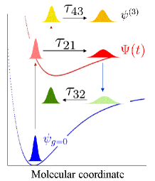
Figure 1: Color online. The pump-dump-pump CARS scheme. $\Psi(t)$ is the desired wavefunction.

The reconstruction of $|\Psi(t)\rangle$ from $P^{(3)}$ proceeds in five steps:

1. Insert a complete set of ground vibrational states. Introducing ${\sum_{g}|\psi_{g}\rangle\langle\psi_{g}|}=\hat{\textbf{1}}$ into Eq. (4) we obtain

$$P^{(3)}(\bm{\tau})=\widetilde{\varepsilon}\sum_{g=0}^{N}e^{-i\widetilde{\omega}_{g}\tau_{32}}P_{g}^{(3)}(\tau_{43},\tau_{21}),$$ (5)

where ${P_{g}^{(3)}(\tau_{43},\tau_{21})=\langle\psi_{0}|e^{-iH_{e}\tau_{43}}|\psi_{g}\rangle\langle\psi_{g}|e^{-iH_{e}\tau_{21}}|\psi_{0}\rangle}$, and ${\widetilde{\omega}_{g}=\omega_{g}-\omega_{0}}$. $N$ is determined by the number of ground vibrational states required to expand $|\Psi(t)\rangle$. Note that the desired correlation functions $c_{g}(t)$ may already be recognized in $P_{g}^{(3)}$.

2. Fourier-transform $P^{(3)}$ with respect to $\tau_{32}$. The transformation resolves $P^{(3)}$ into individual ground-state components, $P_{g}^{(3)}$. Since $\tau_{32}$ is defined to be positive, we multiply Eq. (5), prior to the transformation, by the rectangular function that takes the value 1 for the $\tau_{32}$ domain and 0 elsewhere. Using the Fourier convolution theorem we obtain a sinc-type of spectrum with peaks at the frequencies $\omega=\widetilde{\omega}_{g}$:

$$\widetilde{P}^{(3)}(\tau_{43},\omega,\tau_{21})=\sum_{g=0}^{N}S(\omega,g)P_{g}^{(3)}(\tau_{43},\tau_{21}),$$ (6)

where ${S(\omega,g)=2T\widetilde{\varepsilon}e^{i(\omega-\widetilde{\omega}_{g})(\check{\tau}_{32}+T)}{\rm sinc}[(\omega-\widetilde{\omega}_{g})T]}$, ${2T=\hat{\tau}_{32}-\check{\tau}_{32}}$, and $\check{\tau}_{32}$ ($\hat{\tau}_{32}$) is the minimal (maximal) value of $\tau_{32}$. Fixing $(\tau_{43},\tau_{21})$, Eq. (6) can be written as a matrix equation:

$$\mathbf{\widetilde{P}_{\bm{\omega}}^{(3)}}=\mathbf{S_{\bm{\omega}g}}\mathbf{P_{g}^{(3)}}.$$ (7)

3. Invert the matrix equation (7). The equation $\mathbf{P_{g}^{(3)}}=\mathbf{S_{g\bm{\omega}}^{-1}}\mathbf{\widetilde{P}_{\bm{\omega}}^{(3)}}$ isolates the two-dimensional functions $P_{g}^{(3)}(\tau_{43},\tau_{21})$. In inverting $\mathbf{S}$ we choose the number of frequency elements ($\omega$) equal to the number of the $g$ elements so that the matrix is square. For numerical accuracy, the inversion is implemented separately around each of the peaks at $\widetilde{\omega}_{g}$.

4. Take the square-root of $P_{g}^{(3)}$. Assuming the functions $\{\psi_{g}(x)\}$ are real, we can rewrite $P_{g}^{(3)}$ as

$$P_{g}^{(3)}(\tau_{43},\tau_{21})=\langle\psi_{g}|e^{-iH_{e}\tau_{43}}|\psi_{0}\rangle\langle\psi_{g}|e^{-iH_{e}\tau_{21}}|\psi_{0}\rangle.$$ (8)

Taking the square-root of the diagonal of $P_{g}^{(3)}(\tau_{43},\tau_{21})$ (i.e. ${\tau_{43}=\tau_{21}=t}$), we recover the $c_{g}(t)$ up to a sign:

$$\sqrt{P_{g}^{(3)}(t)}=a_{g}\langle\psi_{g}|e^{-iH_{e}t}|\psi_{0}\rangle\equiv\langle\widetilde{\psi}_{g}|e^{-iH_{e}t}|\psi_{0}\rangle,$$ (9)

where $a_{g}=\pm 1$ and the sign of $\widetilde{\psi}_{g}(x)$ is as yet undetermined. By demanding continuity of the cross-correlation functions (and their derivatives), the coefficients $a_{g}$ can be regarded as time-independent. Substituting Eq. (9) instead of $c_{g}(t)$ into Eq. (3) and using the resulting $C_{g}(t)$ in Eq. (1) yields

$$|\widetilde{\Psi}(t)\rangle=i\mu\varepsilon_{1}\sum_{g=0}^{N}|\psi_{g}\rangle\langle\widetilde{\psi}_{g}|e^{-iH_{e}t}|\psi_{0}\rangle.$$ (10)

The different sign combinations of $\widetilde{\psi}_{g}(x)$ generate $2^{N+1}$ possible superpositions. (In fact, only $2^{N}$ are physically meaningful since we are free to set the sign of one of the $g$-components.) Only one out of the $2^{N}$ $|\widetilde{\Psi}(t)\rangle$ coincides with $|{\Psi}(t)\rangle$: the $|\widetilde{\Psi}(t)\rangle$ for which the sign combination satisfies ${\sum_{g}|\psi_{g}\rangle\langle\widetilde{\psi}_{g}|=\mathbb{1}}$.

5. Discriminating ${|\Psi}(t)\rangle$ from the set $\{|\widetilde{\Psi}(t)\rangle\}$. The set of wavefunctions $\{|\widetilde{\Psi}(t)\rangle\}$ are all consistent with the CARS signal at a specific value of ${\tau_{43}=\tau_{21}}$ footnt . However, only one $|\widetilde{\Psi}(t)\rangle$ is consistent with the signal derivatives. To see this, consider the nth derivative of the experimental signal, Eq. (4), with respect to $\tau_{21}$:

$$\frac{\partial^{n}P^{(3)}(\bm{\tau})}{\partial\tau^{n}_{21}}=\varepsilon^{{\dagger}}\langle\Psi^{*}(\tau_{43})|e^{-iH_{g}\tau_{32}}\widetilde{H}_{e}^{n}|\Psi(\tau_{21})\rangle~{}~{}~{}~{}$$ (11)

$$=\varepsilon^{{\dagger}}\sum_{g,g^{\prime}}e^{-i\omega_{g}\tau_{32}}C_{g}(\tau_{43})C_{g^{\prime}}(\tau_{21})\widetilde{H}_{e,gg^{\prime}}^{n},$$

where $\varepsilon^{{\dagger}}=(-i)^{n-1}\mu^{2}\varepsilon_{1}^{-1}\varepsilon_{2}\varepsilon_{3}e^{i\omega_{0}\tau_{41}}$, $\tau_{41}=\tau-\tau_{1}$, ${\widetilde{H}_{e}^{n}=(H_{e}-\omega_{0}})^{n}$, and ${\widetilde{H}_{e,gg^{\prime}}^{n}=\langle\psi_{g}|\widetilde{H}_{e}^{n}|\psi_{g^{\prime}}\rangle}$. Substituting $|\widetilde{\Psi}(t)\rangle$ instead of $|\Psi(t)\rangle$, into Eq. (11) gives

$$\frac{\partial^{n}\widetilde{P^{(3)}}(\bm{\tau})}{\partial\tau_{21}^{n}} = \varepsilon^{{\dagger}}\sum_{g,g^{\prime}}e^{-i\omega_{g}\tau_{32}}a_{g}a_{g^{\prime}}C_{g}(\tau_{43})C_{g^{\prime}}(\tau_{21})\widetilde{H}_{e,gg^{\prime}}^{n}.$$

Accordingly, the $|\widetilde{\Psi}(t)\rangle$ for which ${\frac{\partial^{n}\widetilde{P^{(3)}}(\bm{\tau})}{\partial\tau_{21}^{n}}=\frac{\partial^{n}P^{(3)}(\bm{\tau})}{\partial\tau_{21}^{n}}}$ for all $n$, is the wavefunction that coincides with $|\Psi(t)\rangle$ of Eq. (2), and hence, is the reconstruction solution.

In practice, we proceed as follows. We invert the time-dependent Schrödinger equation to calculate a set of potentials from each $|\widetilde{\Psi}(t)\rangle$:

$$V(x) = \frac{1}{\widetilde{\Psi}(x,t)}\left[i\frac{\partial}{\partial t}+\frac{1}{2m}\frac{\partial^{2}}{\partial x^{2}}\right]\widetilde{\Psi}(x,t),~{}~{}~{}$$ (13)

where $m$ is the system’s reduced mass. One can show that the potentials calculated by the $|\widetilde{\Psi}(t)\rangle$ that do not coincide with $|\Psi(t)\rangle$, are time-dependent avisar . Only the potential calculated with $|\widetilde{\Psi}(t)\rangle=|\Psi(t)\rangle$ is time-independent and hence corresponds to the excited-state Hamiltonian $H_{e}$ of the measured system. Thus, in order to find the correct wavefunction we use the set of calculated potentials, as if they were time-independent, to propagate the corresponding $\{|\widetilde{\Psi}(t)\rangle\}$ back to time zero. Of all the potentials, only the truly time-independent one will propagate the corresponding $|\widetilde{\Psi}(t)\rangle$ correctly back to $|\psi_{0}\rangle$, and therefore this $|\widetilde{\Psi}(t)\rangle$ is the correct wavefunction. Note that the above procedure requires knowing the signal as a function only of $\tau_{32}$ and $\tau_{21}=\tau_{43}$.

Table 1: The parameters, in atomic units, for the $X$, $A$ and $\widetilde{A}$ potentials used in simulating the CARS signals.

	$X$	$A$	$\widetilde{A}$
$D$	0.0378492	0.0426108	9.11267$\times 10^{-5}$
$b$	0.4730844	0.3175063	1.5875317
$x_{0}$	5.0493478	5.8713786	7.3699313
$T$	0	0.0640074	0.0640074

To test the above reconstruction methodology, we simulated the CARS signal by calculating ${\langle\psi^{(0)}(\tau)|\hat{\mu}|\psi^{(3)}(\tau)\rangle}$ as a function of the three time-delays, for two one-dimensional systems. The first is the Li₂ molecule, with its ground ($X$) and first-excited ($A$) electronic states as Morse-type potentials, ${V(x)=D(1-e^{-b(x-x_{0})})^{2}+T}$. The second system, henceforth denoted d-Li₂, has the Li₂ ground state ($X$) but a dissociative excited potential of the form ${V(x)=De^{-b(x-x_{0})}+T}$ (denoted $\widetilde{A}$). Table 1 gives the potential parameters in atomic units used for the simulations. The parameters for the Morse-type potentials are based on data published in herzberg .

The wavepacket propagations employed in simulating $P^{(3)}$ were performed using the split-operator method feit on a spatial grid of 256 points in the range of $2$–$12$a.u. with time spacing of $\Delta t$=0.1fs. A constant transition-dipole of $2$a.u. was used, and the pulse amplitudes $\varepsilon_{1,2,3}$ were taken to be $10^{-4}$a.u. The ranges of time-delay for the Li₂ (d-Li₂) system were $\tau_{21,43}=0-200$fs ($0-80$fs) with spacing of $0.2$fs. For both systems, we took $\tau_{32}=3-6000$fs with $1$fs spacing.

For Li₂, we inverted Eq. (7) for each of the first 25 peaks of $\widetilde{P}^{3}(\omega)$ using the matrices $\mathbf{S}$ with 25 frequency grid points centered around the peaks at $\widetilde{\omega}_{g}$. This produced 25 two-dimensional functions $P_{g}^{(3)}$, $g=0,\ldots,24$. For d-Li₂ the procedure was performed for the first 40 peaks, producing 40 two-dimensional functions $P_{g}^{(3)}$, $g=0,\ldots,39$.

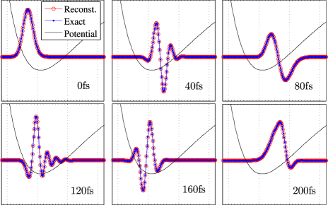
Figure 2: Color online. Snapshots of the real part of the reconstructed (circles, red) vs. the exact (dots, blue) wavefunction, at various times on the excited ($A$) potential (solid line) of Li₂.

In Figs. 2 and 3 we present snapshots of the real part of the reconstructed first-order wavefunction for the Li₂ and the d-Li₂ molecules, respectively. For Li₂ (d-Li₂) we superpose the first 25 (40) eigenfunctions $\psi_{g}(x)$ using the cross-correlation functions obtained by the CARS analysis and maintaining $\sum_{g}|\psi_{g}\rangle\langle\widetilde{\psi}_{g}|=\mathbb{1}$.

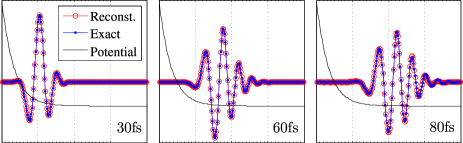
Figure 3: Color online. Snapshots of the real part of the reconstructed (circles, red) vs. the exact (dots, blue) wavefunction, at various times on the excited ($\widetilde{A}$) potential (solid line) of d-Li₂.

The reconstructed wavefunctions are seen to be in excellent agreement with the exact ones, obtained by direct calculation of the first-order population, for all propagation times. For the Li₂ system, a high quality reconstruction is already obtained by superposing just 20 basis functions.

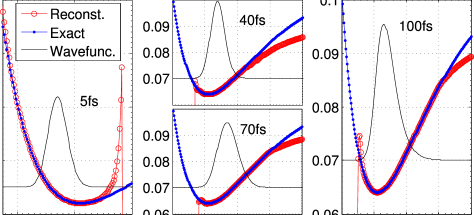
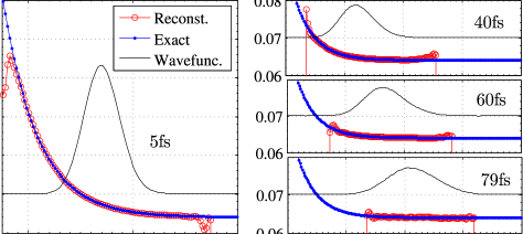
Figure 4: Color online. The reconstructed (circles, red) vs. the exact (dots, blue) $A$ potential of Li₂.

Figure 5: Color online. The reconstructed (circles, red) vs. the exact (dots, blue) $\widetilde{A}$ potential of d-Li₂.

Having determined the wavefunctions we calculate the corresponding excited potential surfaces from Eq. (13) using eight-point (three-point) central finite-differencing for the time (spatial) derivatives. The time-step used was 0.2fs but very good results were also obtained using 0.5fs. Figures 5 and 5 compare the reconstructed vs. the exact potentials. The wavefunction (absolute value) used in calculating the potential is shown by a black solid line. Note from Figs. 5 and 5 that combining the reconstructed potential from two points in time (e.g. $5$ and $70$fs for Li₂ and $5$ and $79$fs for d-Li₂) is sufficient to reconstruct the potential over the full range of interest (2–5Å). Once the potential is known one can calculate the excited-state wavefunction as a function of time for any excitation pulse sequence without the need for any additional laboratory experiments.

To conclude, we have presented a methodology for the complete reconstruction of the excited-state wavefunction of a reacting molecule by analyzing a multi-dimensional resonant CARS signal. The methodology applies to polyatomics as well as diatomics. We have assumed that only the ground-state potential is known. The approach is very compelling since the desired excited-state wavefunction is explicitly contained in the formula for the CARS signal. Highly accurate reconstruction is obtained even far from the Franck-Condon region. In fact, in practice the method may be more accurate far from the Franck-Condon region, since the frequency shift between the pump and dump pulses will be more effective in discriminating unwanted processes that may contribute to the measured signal at $\mathbf{k=k_{1}-k_{2}+k_{3}}$. We simplified matters by considering $\delta$-function pulse excitations, a coordinate-independent transition dipole moment and only one excited-state potential. In future work we will test the removal of all these assumptions.

We have shown that once the time-dependent wavefunction is found, the excited potential can be reconstructed with quite high accuracy. It will be of great interest to test the method on polyatomics, where obtaining multidimensional potential surfaces from spectroscopic data has been one of the longstanding challenges of molecular spectroscopy. An important application of excited-state potential reconstruction will be the ab initio simulations of laser control of chemical bond breaking. Experimental laser control has been greatly hindered by the lack of detailed theoretical guidance, which in turn is due to the lack of accurate excited-state potentials. The present methodology could have a significant impact in this field by providing the necessary information about excited-state potentials.

This research was supported by the Minerva Foundation and made possible, in part, by the historic generosity of the Harold Perlman family.

Supplementary Online Material – Determining the Correct Wavefunction out of the Set $\{\widetilde{\Psi}_{i}(t)\}$

In this supplement we explain how we determine the correct wavefunction out of the set of wavefunctions $\{\widetilde{\Psi}_{i}(t)\}$, $i=1,2,...,2^{N}$, where $N$ is the number of basis functions $\{\psi_{g}\}$ needed to span $\Psi(t)$ (ref [22] in the paper).

We have defined a set of wavefunctions that can be constructed using the information obtained from the CARS signal:

$$|\widetilde{\Psi}(t)\rangle \equiv \sum_{g}|\psi_{g}\rangle\langle\widetilde{\psi}_{g}|e^{-iH_{e}t}|\psi_{0}\rangle$$ (14)

$$= \sum_{g}|\psi_{g}\rangle\langle\widetilde{\psi}_{g}|\Psi(t)\rangle\equiv\widetilde{\mathbb{1}}|\Psi(t)\rangle.$$

(In writing Eq. (14) we omitted the proportionality coefficient $i\mu\varepsilon_{1}$ relative to Eq. (10) in the paper.) Recall that $\widetilde{\mathbb{1}}\equiv\sum_{g}|\psi_{g}\rangle\langle\widetilde{\psi}_{g}|\equiv\sum_{g}|\psi_{g}\rangle a_{g}\langle\psi_{g}|$ where $a_{g}$ may take one out of two possible values: $\pm 1$. A useful property of the operator $\widetilde{\mathbb{1}}$ is that its square equals the identity operator $\mathbb{1}$:

$$\widetilde{\mathbb{1}}\widetilde{\mathbb{1}} = \sum_{gg^{\prime}}a_{g}a_{g^{\prime}}|\psi_{g}\rangle\langle\psi_{g}|\psi_{g^{\prime}}\rangle\langle\psi_{g^{\prime}}|$$ (15)

$$= \sum_{g}a^{2}_{g}|\psi_{g}\rangle\langle\psi_{g}|=\sum_{g}|\psi_{g}\rangle\langle\psi_{g}|=\mathbb{1}.$$

We can derive an equation of motion for $\widetilde{\Psi}(t)$:

$$\frac{\partial}{\partial t}|\widetilde{\Psi}(t)\rangle = \frac{\partial}{\partial t}\widetilde{\mathbb{1}}|\Psi(t)\rangle=\widetilde{\mathbb{1}}\frac{\partial}{\partial t}|\Psi(t)\rangle=-i\widetilde{\mathbb{1}}H_{e}|\Psi(t)\rangle$$ (16)

$$= -i\widetilde{\mathbb{1}}H_{e}\widetilde{\mathbb{1}}\widetilde{\mathbb{1}}|\Psi(t)\rangle=-i\widetilde{\mathbb{1}}H_{e}\widetilde{\mathbb{1}}|\widetilde{\Psi}(t)\rangle$$

$$\equiv -i\widetilde{H}_{e}|\widetilde{\Psi}(t)\rangle,$$

where, we have used the fact that $\widetilde{\mathbb{1}}$ is time-independent and therefore commutes with $\frac{\partial}{\partial t}$. Equation (16) shows that $\widetilde{\Psi}(t)$ obeys a time-dependent Schrödinger equation with the effective Hamiltonian $\widetilde{H}_{e}=\widetilde{\mathbb{1}}H_{e}\widetilde{\mathbb{1}}$.

The Hamiltonian $H_{e}$ has the conventional form of $H_{e}=V_{e}+T$, where $T$ is the kinetic-energy operator. The Hamiltonian $\widetilde{H}_{e}$ therefore takes the form:

$$\widetilde{H}_{e}\equiv\widetilde{\mathbb{1}}H_{e}\widetilde{\mathbb{1}}=\widetilde{\mathbb{1}}V_{e}\widetilde{\mathbb{1}}+\widetilde{\mathbb{1}}T\widetilde{\mathbb{1}}\equiv\widetilde{V}_{e}+\widetilde{T},$$ (17)

Note that the operator $\widetilde{\mathbb{1}}$ does not commute with $V_{e}$, $T$ or $H_{e}$ since it does not share a common basis of eigenvectors with the last three operators. Note also that the operators $\widetilde{V}_{e}$, $\widetilde{T}$ and $\widetilde{H}_{e}$ are all time-independent.

Rearranging Eq. (16), we obtain:

$$\widetilde{V}_{e} = \frac{1}{\widetilde{\Psi}(t)}\left[i\frac{\partial}{\partial t}-\widetilde{T}\right]\widetilde{\Psi}(t).$$ (18)

where we emphasize that $\widetilde{V}_{e}$ is time-independent. Let us now define the related quantity

$$V = \frac{1}{\widetilde{\Psi}(t)}\left[i\frac{\partial}{\partial t}-T\right]\widetilde{\Psi}(t),$$ (19)

where $T$ is the usual kinetic energy operator. Obviously, for $\widetilde{\Psi}(t)\equiv\Psi(t)$ Eq. (19) is equivalent to the usual time-dependent Schrödinger equation for $\Psi(t)$ and therefore $V\equiv V_{e}$ is time-independent. We claim that for any other, incorrect, wavefunction $\widetilde{\Psi}(t)$, Eq. (19) results in a time-dependent potential $V$.

In order to show this we substitute $\widetilde{T}=T+\Delta T$ in Eq. (18), where $\Delta T=\widetilde{T}-T$, and obtain:

$$\widetilde{V}_{e} = \frac{1}{\widetilde{\Psi}(t)}\left[i\frac{\partial}{\partial t}-(T+\Delta T)\right]\widetilde{\Psi}(t)$$ (20)

$$= V-\frac{1}{\widetilde{\Psi}(t)}\left[\Delta T\right]\widetilde{\Psi}(t).$$

The term $\frac{1}{\widetilde{\Psi}(t)}[\Delta T]\widetilde{\Psi}(t)$ is time-dependent (unless $\widetilde{\Psi}(t)$ is an eigenfunction of $\Delta T$, which has no general reason to hold. In addition, in the Appendix we show that $\Delta T$ is generally different from zero). Therefore, in order to preserve the time-independence of $\widetilde{V}_{e}\equiv\widetilde{\mathbb{1}}V_{e}\widetilde{\mathbb{1}}$, $V$ must also be time-dependent.

To summarize: in order to determine the correct wavefunction out of the set of wavefunctions $\{\widetilde{\Psi}_{i}(t)\},i=1,2,...,2^{N}$, we use the fictitious Schrödinger equation, (19), to calculate a potential, $V$, from each wavefunction $\widetilde{\Psi}(t)$ of the set. At different times, $t$, the wavefunctions $\widetilde{\Psi}(t)$ will give different potentials $V$ except for the one correct wavefunction, $\Psi(t)$, that corresponds to the correct Schrödinger equation and therefore will give the same potential, $V\equiv V_{e}$, at all times. Thus, the correct wavefunction $\Psi(t)$ can be selected from the set $\{\widetilde{\Psi}_{i}(t)\}$ as the one that provides a time-independent potential via Eq. (19). Alternatively, as described in the paper, the wavefunction $\widetilde{\Psi}(t)$ that propagates back to the known $\Psi(0)\equiv\psi_{0}$, using the corresponding potential calculated by Eq. (19), is guaranteed to be the correct reconstructed wavefunction, $\Psi(t)$.

.1 Appendix

We show that $\Delta T\neq 0$:

$$\Delta T = (\widetilde{T}-T)=\widetilde{\mathbb{1}}\widetilde{\mathbb{1}}(\widetilde{\mathbb{1}}T\widetilde{\mathbb{1}}-T)$$ (21)

$$= \widetilde{\mathbb{1}}(T\widetilde{\mathbb{1}}-\widetilde{\mathbb{1}}T)=\widetilde{\mathbb{1}}[T,\widetilde{\mathbb{1}}].$$

The commutator $[T,\widetilde{\mathbb{1}}]$ is not identically zero. Therefore, $\widetilde{\mathbb{1}}[T,\widetilde{\mathbb{1}}]\equiv\Delta T$ is not identically zero as well.