First-order virial expansion of short-time diffusion and sedimentation coefficients of permeable particles suspensions

Abstract

For suspensions of permeable particles, the short-time translational and rotational self-diffusion coefficients, and collective diffusion and sedimentation coefficients are evaluated theoretically. An individual particle is modeled as a uniformly permeable sphere of a given permeability, with the internal solvent flow described by the Debye-Bueche-Brinkman equation. The particles are assumed to interact non-hydrodynamically by their excluded volumes. The virial expansion of the transport properties in powers of the volume fraction is performed up to the two-particle level. The first-order virial coefficients corresponding to two-body hydrodynamic interactions are evaluated with very high accuracy by the series expansion in inverse powers of the inter-particle distance. Results are obtained and discussed for a wide range of the ratio, $x$, of the particle radius to the hydrodynamic screening length inside a permeable sphere. It is shown that for $x\gtrsim 10$, the virial coefficients of the transport properties are well-approximated by the hydrodynamic radius (annulus) model developed by us earlier for the effective viscosity of porous-particle suspensions.

I Introduction

One of the theoretical methods to analyze transport properties in suspensions of interacting colloidal particles is the virial expansion in terms of the particle volume fraction $\phi$. For suspensions of non-permeable hard spheres with stick hydrodynamic boundary conditions, virial expansion results for short-time properties are known to high numerical precision up to the three-particle level, i.e., to quadratic order in $\phi$ for diffusion and sedimentation coefficients CEW:99 ; Cichocki:02 , and to third order in $\phi$ for the effective viscosity Cichocki:03 . The concentration range of applicability of these hard-sphere virial expansion results in comparison to simulation data has been discussed in BanchioASD:08 . Our knowledge on virial expansion coefficients of colloidal transport properties is less developed when suspensions of solvent-permeable particles are considered. The theoretical description of their dynamics is more complicated since one needs to account for the solvent flow also inside the particles. Permeable particle systems are frequently encountered in soft matter science. Prominent examples of practical relevance which are the subject of ongoing research, are dendrimers Likos:02 ; Likos:2010 , microgel particles Pyett:05 ; Richtering:08 ; Coutinho2008 , a large variety of core-shell particles with a dry core and an outer porous layer Nommensen:01b ; Petekidis:04 ; Zackrisson:05 ; Adamczyk2004 ; Malysa , fractal aggregates Saarloos:87 , and star-like polymers of lower functionality LikosRichter:98 .

In a series of recent articles Abade-JCP:10 ; ACENW-trans-PRE:10 ; ACENW-visco-JCP:10 ; ACENW-visco-JPCM:10 , we have explored the generic effect of solvent permeability on the short-time transport using the model of uniformly permeable colloidal spheres with excluded volume interactions. This simple model is specified by two parameters only, namely the particle volume fraction $\phi=(4\pi/3)na^{3}$, where $n$ is the number concentration and $a$ is the particle radius, and the ratio $x$ of the particle radius to the hydrodynamic penetration depth inside a permeable sphere. Large (low) values of $x$ correspond to weakly (strongly) permeable particles. While the model of uniformly permeable hard spheres ignores a specific intra-particle structure, it is generic in the sense that the hydrodynamic structure of more complex porous particles can be approximately accounted for in terms of a mean permeability. In our related previous publications, using a hydrodynamic multipole simulation method of a very high accuracy CFHWB:94 , encoded in the hydromultipole program package CEW:99 , we have calculated the short-time translational diffusion properties Abade-JCP:10 ; ACENW-trans-PRE:10 , and the high-frequency viscosity ACENW-visco-JCP:10 ; ACENW-visco-JPCM:10 of the permeable spheres model, as functions of $\phi$ and $x$. These results cover the full range of permeabilities, with volume fractions extending up to the liquid-solid transition.

While the simulation results are important for the general understanding of permeability effects in concentrated systems, for practical use in experimental data evaluation and as input in long-time theories, virial expansion results based on a rigorous theoretical calculation are still strongly on demand. In fact, the knowledge of the leading-order virial coefficients can be a good starting point in deriving approximate expressions for transport properties, which may be applicable at concentrations much higher than those where the original (truncated) virial expansion result is useful. An example in case is provided in our recent derivation ACENW-visco-JPCM:10 of a generalized Saitô expression for the effective high-frequency viscosity $\eta_{\infty}$ of permeable spheres, based on the second-order concentration expansion result, i.e. a Huggins coefficient calculation, of this property.

In ACENW-visco-JCP:10 , we have performed virial expansion calculations for $\eta_{\infty}$. We have investigated therein a simplifying hydrodynamic radius model (HRM), where a uniformly permeable sphere of radius $a$ is described by a spherical annulus particle with an inner hydrodynamic radius $a_{\text{eff}}(x)<a$, and unchanged excluded-volume radius $a$. In this annulus model (HRM), the Huggins coefficient describing two-body viscosity contributions has been evaluated and shown to be in a remarkably good agreement with the precise numerical data for porous particles, characterized by a wide range of permeabilities realized in experimental systems.

In the present article, the aforementioned theoretical work on the virial expansion of the high-frequency viscosity is generalized to short-time diffusion properties. In Sec. II, the virial expansion is performed for the translational and rotational self-diffusion coefficients $D_{t}$ and $D_{r}$, respectively, the sedimentation coefficient $K$, and the associated collective diffusion coefficient $D_{C}=KD_{0}^{t}/S(0)$. Here, $S(0)$ is the small-wavenumber limit of the static structure factor, and $D_{0}^{t}$ is the single-particle translational diffusion coefficient. In Sec. III, we provide highly accurate numerical values for the first-order (i.e., two-particle) virial coefficients, $\lambda_{t}(x)$, $\lambda_{r}(x)$, $\lambda_{C}(x)$ and $\lambda_{K}(x)$, of $D_{t}$, $D_{r}$, $D_{C}$ and $K$, respectively, in the full range of permeabilities. In Sec. IV, we also recalculate these virial coefficients approximately on the basis of the simplifying annulus model (HRM). In Sec. V, we conclude that in the range $x\gtrsim 10$ typical of many permeable particle systems, the virial coefficients are well approximated by the annulus model.

II Theory

We consider a suspension made of a fluid with shear viscosity $\eta_{0}$ and identical porous particles of radius $a$. The fluid flow is characterized by Reynolds number Re$<<1$. Outside the particles, the fluid velocity ${\bm{v}}$ and pressure $p$ satisfy the Stokes equations Kim-Karrila:1991 ; Happel-Brenner:1986 ,

$$\eta_{0}\;\!{\bm{\nabla}}^{2}{\bm{v}}({\bm{r}})-{\bm{\nabla}}p({\bm{r}}) = 0$$

$${\bm{\nabla}}\cdot{\bm{v}}({\bm{r}}) = 0,$$ (1)

and inside the particles, the Debye-Büche-Brinkman (DBB) equations Brinkman:47d ; DebyeBueche:48 ,

$$\eta_{0}\;\!{\bm{\nabla}}^{2}{\bm{v}}({\bm{r}})-\eta_{0}\;\!\kappa^{2}\left[{\bm{v}({\bm{r}})}-{\bm{u}}_{i}({\bm{r}})\right]-{\bm{\nabla}}p({\bm{r}}) = 0$$

$${\bm{\nabla}}\cdot{\bm{v}}({\bm{r}}) = 0,$$ (2)

where $\kappa^{-1}$ is the hydrodynamic penetration depth. The skeleton of the particle $i$, centered at ${\bf r}_{i}$, moves rigidly with the local velocity ${\bf u}_{i}({\bf r})={\bf U}_{i}+{\bm{\omega}}_{i}\times\left({\bf r}-{\bf r}_{i}\right)$, determined by the translational and rotational velocities ${\bf U}_{i}$ and ${\bm{\omega}}_{i}$ of the particle $i$, respectively. The fluid velocity and stress tensor are continuous across a particle surface. The effect of the particle porosity is therefore described by the ratio $x$ of the particle radius $a$ to the hydrodynamic screening length $\kappa^{-1}$ of the porous material inside the particle, i.e.

$$x = \kappa a.$$ (3)

Owing to linearity of the Stokes and DBB equations and the boundary conditions, the particle velocity $\mathbf{U}_{i}$ depends linearly on the external forces $\mathbf{F}_{j}$ exerted on a particle $j$. In particular, for two interacting spherical particles, $1,2$, in the absence of external torques and flows,

$$\mathbf{U}_{1} = \bm{\mu}_{11}^{tt}({\bf r}_{1},{\bf r}_{2})\cdot\mathbf{F}_{1}+\bm{\mu}_{12}^{tt}({\bf r}_{1},{\bf r}_{2})\cdot\mathbf{F}_{2}$$ (4)

$$\mathbf{U}_{2} = \bm{\mu}_{21}^{tt}({\bf r}_{1},{\bf r}_{2})\cdot\mathbf{F}_{1}+\bm{\mu}_{22}^{tt}({\bf r}_{1},{\bf r}_{2})\cdot\mathbf{F}_{2}.$$ (5)

In this paper, the two-particle translational-translational mobility matrices $\bm{\mu}_{ij}^{tt}({\bf r}_{1},{\bf r}_{2})$ are evaluated using the multipole method of solving the Stokes an DBB equations CFHWB:94 . The cluster expansion of the above mobility matrices reads,

$$\bm{\mu}_{ij}^{tt}({\bf r}_{1},{\bf r}_{2})=\mu_{0}^{t}\delta_{ij}\mathbf{1}+\bm{\mu}_{ij}^{tt(2)}(\mathbf{r}),$$ (6)

where $\mathbf{r}=\mathbf{r}_{2}-\mathbf{r}_{1}$ and

$$\mu_{0}^{t}=\frac{1}{4\pi\eta_{0}A_{10}}$$ (7)

is the single porous-particle translational mobility. Here $A_{10}$ is a single porous-particle scattering coefficient Cichocki_Felderhof_Schmitz:88 , given explicitly in Appendix A. For a non-permeable hard sphere with stick boundary conditions, $A_{10}^{\text{hs}}={3a}/{2}$.

The single particle scattering coefficients $A_{l\sigma}$, with $l=1,2,3,4,...$ and $\sigma=1,2,3$  Cichocki_Felderhof_Schmitz:88 , are essential to perform the multipole expansion. They determine the corresponding multipoles of the hydrodynamic force density on a particle immersed in an ambient flow; examples are Eqs. (7) and (26). The same coefficients $A_{l\sigma}$ specify also the corresponding multipoles of the fluid velocity, reflected (scattered) by a particle immersed in a given ambient flow. This is why $A_{l\sigma}$ are called “scattering coefficients”. In the multipole approach, differences in the internal structure of particles (e.g. solid, liquid, gas, porous, core-shell, stick-slip), are fully accounted by different scattering coefficients. The other parts of the multipole algorithm need not to be changed. The scattering coefficients are the matrix elements of two single-particle friction operators, ${\bf Z}_{0}$ and $\hat{\bf Z}_{0}$, which determine the hydrodynamic force density exerted by a given ambient flow on a motionless and a freely moving particle, respectively.

In the multipole expansion method, the two-particle mobility $\bm{\mu}^{(2)}(1,2)$ (e.g. translational one, as in Eq. (6), or rotational one, as in Eq. (25)) is expressed in terms of the single-particle friction operators, ${\bf Z}_{0}(i)$ and $\hat{\bf Z}_{0}(i)$, with $i=1,2$, and the Green operator ${\bf G}(1,2)$. The later relates the flow outgoing from particle 2 and incoming on particle 1. We can write $\bm{\mu}^{(2)}$ as an infinite scattering series,

$$\mbox{\boldmath$\mu$}^{(2)} = \mbox{\boldmath$\mu$}_{0}{\mathbf{Z}}_{0}(1+{\bf G}\hat{{\mathbf{Z}}}_{0})^{-1}{\bf G}{\mathbf{Z}}_{0}\mbox{\boldmath$\mu$}_{0}$$ (8)

$$= \mbox{\boldmath$\mu$}_{0}{\mathbf{Z}}_{0}{\bf G}{\mathbf{Z}}_{0}\mbox{\boldmath$\mu$}_{0}-\mbox{\boldmath$\mu$}_{0}{\mathbf{Z}}_{0}{\bf G}\hat{{\mathbf{Z}}}_{0}{\bf G}{\mathbf{Z}}_{0}\mbox{\boldmath$\mu$}_{0}+....$$

Since the multipole matrix elements of the Green tensor G scale as inverse powers of the interparticle distance $r$, Eq. (8) corresponds to a power series in $1/r$. Truncating the expansion at order $1/r^{1000}$, we obtain a very high precision of the mobility calculation, actually much higher than needed for any practical applications.

In the present work, we investigate the short-time dynamics, at time scales $t<<a^{2}/D_{0}^{t}$, where

$$D_{0}^{t}=k_{B}T\mu_{0}^{t}$$ (9)

is the single-particle translational diffusion coefficient, with the Boltzmann constant $k_{B}$ and temperature $T$. On the short-time scale, the system is described by the equilibrium particle distribution hansen . In the further analysis, we will need only the small-concentration limit $g_{0}(r)$ of the pair distribution function, where $r$ is the interparticle distance. For particle-particle direct interactions described by a pair potential $V(r)$, this pair distribution is $g_{0}(r)=\exp(-V(r)/k_{B}T)$. For non-overlapping spheres of radius $a$,

$$g_{0}(r) = \left\{\begin{array}[]{ll}0&\mbox{ for }\;r\leq 2a,\\ 1&\mbox{ for }\;r>2a.\end{array}\right.$$ (12)

The first-order terms in the virial expansion of the short-time transport coefficients are obtained by averaging the corresponding two-particle mobility elements. As the result, the virial coefficients are obtained as integrals, which involve the mobility elements and $g_{0}(r)$.

The first-order virial expansion of the short-time translational self-diffusion coefficient has the form,

$$D_{t}=D_{0}^{t}(1+\lambda_{t}\phi+{\cal O}(\phi^{2})).$$ (13)

The coefficient $\lambda_{t}$ is given by the relation Cichocki_Felderhof:88 ,

$$\lambda_{t}=8\int_{1}^{+\infty}g_{0}(R)J_{t}(R)R^{2}dR,$$ (14)

with $\mathbf{R=r/}2a$ and

$$J_{t}(R)=\frac{1}{\mu_{0}^{t}}\mbox{Tr}\,\bm{\mu}_{11}^{tt(2)}(\mathbf{r}).$$ (15)

Here, Tr denotes the trace operation. For the sedimentation coefficient, one obtains,

$$K=1+\lambda_{K}\phi+...$$ (16)

where

$$\lambda_{K} = \frac{2}{5a^{3}}A_{12}+\frac{8}{a}A_{10}\int_{0}^{+\infty}\left[g_{0}(R)-1\right]RdR$$ (18)

$$+8\int_{1}^{+\infty}g_{0}(R)J_{K}(R)R^{2}dR,$$

and

$$J_{K}(R)=\frac{1}{\mu_{0}^{t}}\mbox{Tr}\left[\bm{\mu}_{11}^{tt(2)}(\mathbf{r})+\bm{\mu}_{12}^{tt(2)}(\mathbf{r})-\mathbf{T}_{0}(\mathbf{r)}\right].$$ (19)

In the above expression,

$$\mathbf{T}_{0}(\mathbf{r)=}\frac{\mathbf{1+}\widehat{\mathbf{r}}\widehat{\mathbf{r}}}{8\pi\eta_{0}r},$$ (20)

is the Oseen tensor and $\widehat{\mathbf{r}}=\mathbf{r/}r$.

The scattering coefficient $A_{12}$ for a porous particle Cichocki_Felderhof_Schmitz:88 is given explicitly in Appendix A. For a non-permeable hard sphere with the stick boundary conditions, $A_{12}^{\text{hs}}={5a^{3}}/{2}$.

The collective diffusion coefficient is given by

$$D_{C}=D_{0}^{t}K/S(0),$$ (21)

where $S(0)$ is the zero-wavenumber limit of the static structure factor, $S(0)=\lim_{q\rightarrow 0}S(q)$. The first-order virial expansion of Eq. (21) has the form,

$$D_{C} = D_{0}^{t}(1+\lambda_{C}\phi+...).$$ (22)

For the non-overlapping spheres hansen ,

$$S(0)=1-8\phi+{\cal O}(\phi^{2}).$$ (23)

In this case,

$$\lambda_{C}=\lambda_{K}+8.$$ (24)

The relation (24) follows from Eqs. (16), (21) and (22).

We proceed by analyzing the short-time rotational self-diffusion coefficient. In the absence of external forces and flows, the two-particle rotational-rotational mobility matrices $\bm{\mu}_{ij}^{rr}({\bf r}_{1},{\bf r}_{2})$ satisfy the relation analogical to Eqs. (4)-(5), with the translational velocities replaced by the rotational ones, and the forces replaced by the torques. The two-particle cluster expansion now reads,

$$\bm{\mu}_{ij}^{rr}({\bf r}_{1},{\bf r}_{2})=\mu_{0}^{r}\delta_{ij}\mathbf{1}+\bm{\mu}_{ij}^{rr(2)}(\mathbf{r}),$$ (25)

with

$$\mu_{0}^{r}=\frac{1}{8\pi\eta_{0}A_{11}}.$$ (26)

The scattering coefficient $A_{11}$ for a porous particle Cichocki_Felderhof_Schmitz:88 is given in Appendix A. For a non-permeable hard sphere with the stick boundary conditions, ${A_{11}^{\text{hs}}}={a^{3}}$.

The virial expansion of the rotational self-diffusion coefficient is

$$D_{r}=D_{0}^{r}(1+\lambda_{r}\phi+...),$$ (27)

where

$$D_{0}^{r}=k_{B}T\mu_{0}^{r}$$ (28)

and

$$\lambda_{r}=8\int_{1}^{+\infty}g_{0}(R)J_{r}(R)R^{2}dR,$$ (29)

with

$$J_{r}(R)=\frac{1}{\mu_{0}^{r}}\mbox{Tr}\,\bm{\mu}_{11}^{rr(2)}(\mathbf{r}).$$ (30)

III Results

To evaluate the first order virial coefficients $\lambda\!=\!\lambda_{t},\lambda_{K},\lambda_{r}$, we calculate two-particle mobility matrix elements, performing a series expansion in powers of $1/r$ up to the order 1000, as described in Sec. II. Integration with respect to the particle positions has been performed analytically term by term, using the expressions given in the previous section. The virial coefficients $\lambda$ have been evaluated for a wide range of $x$. Selected results are listed in Table 1. All displayed digits are significant. (More data are available on request.)

Table 1: First virial coefficients $\lambda_{t}$, $\lambda_{K}$ and $\lambda_{r}$ for the short-time translational self-diffusion, sedimentation and rotational self-diffusion, respectively.

$x$	$\lambda_{t}$	$\lambda_{K}$	$\lambda_{r}$
3	-0.2497	-3.4451	-0.03257
4	-0.4159	-4.1066	-0.06336
5	-0.5692	-4.5539	-0.09682
6	-0.7021	-4.8722	-0.12956
7	-0.8149	-5.1084	-0.16012
8	-0.9102	-5.2898	-0.18802
9	-0.9909	-5.4328	-0.21327
10	-1.0598	-5.5480	-0.23606
11	-1.1190	-5.6426	-0.25662
13	-1.2151	-5.7884	-0.29208
16	-1.3202	-5.9380	-0.33426
18	-1.3730	-6.0095	-0.35692
20	-1.4161	-6.0662	-0.37628
30	-1.5499	-6.2335	-0.44202
40	-1.6190	-6.3149	-0.48007
50	-1.6610	-6.3628	-0.50497
65	-1.7001	-6.4064	-0.52959
100	-1.7460	-6.4563	-0.56075
$\infty$	-1.8315	-6.5464	-0.63054

In Fig. 1, the first order viral expansion of the short-time translational self-diffusion coefficient of a porous-particle suspension is compared with the accurate simulation results performed in Ref. Abade-JCP:10 for volume fractions $\phi\leq 0.45$. The first order virial expansion, see Eq. (13), can be used as an accurate approximation of $D_{t}$ in a very wide range of volume fractions, even for relatively large values of $x$ (i.e. low permeabilities).

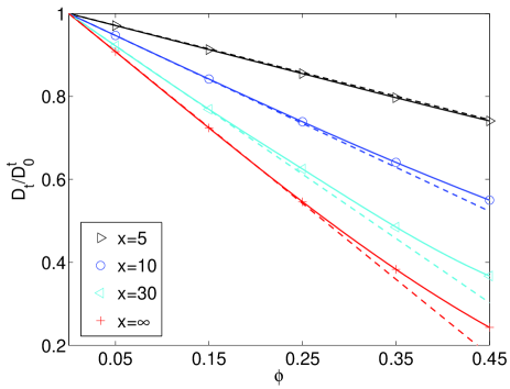
Figure 1: Translational self-diffusion coefficient $D_{t}$ for a suspension of porous particles. Symbols connected by splines (solid lines): accurate simulation results from Ref. Abade-JCP:10 . Dashed straight lines: first-order virial expansion calculated in this work.

In contrast, values of the sedimentation coefficient $K$ differ significantly from the first-order virial estimation already at rather small volume fractions, see Ref. Abade-JCP:10 . Our values of $\lambda_{K}(\infty)$ reproduce with a higher accuracy the classic Batchelor’s result BatchelorSedimentation:72 for non-permeable hard spheres. For uniformly porous particles, the boundary collocation method was applied by Chen and Cai Chen_Cai:99 to evaluate $\lambda_{K}=-3.46,\;-5.50,\;-6.23,\;-6.44$ for $x^{2}=10^{\alpha}$, with $\alpha=1,2,3,4$, respectively. Comparing their results with our very accurate values, $\lambda_{K}=-3.5723,\;-5.5480,\;-6.2504,\;-6.4563$, we conclude that the uncertainty of their results is decreasing from 3% at $\alpha=1$ to 0.3% at $\alpha=4$. The accuracy of the boundary collocation method is worse at smaller values of $x$, i.e. for larger permeabilities.

In Figs. 2-4, the first-order virial coefficients $\lambda$ are plotted versus the porosity parameter $1/x$, for $1/x\leq 0.1$, i.e. for $x\geq 10$. For $1/x=0$, i.e. for $x=\infty$, the limit of a non-permeable hard sphere with radius $a$ is recovered, $\lambda^{\text{hs}}=\lambda(\infty)$.

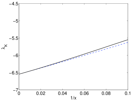
Figure 2: Two-particle sedimentation virial coefficient $\lambda_{K}(x)$. Our precise results for porous particles (solid line) are well-approximated by the annulus model (dashed line).

As shown in Fig. 2, for a low permeability, the coefficient $\lambda_{K}~{}\approx~{}\lambda_{K}^{\text{hs}}~{}+~{}10/x$ is approximately a linear function of $1/x$. The coefficients $\lambda_{t}$ and $\lambda_{r}$ as functions of $1/x$ are shown in Figs. 3 and 4.

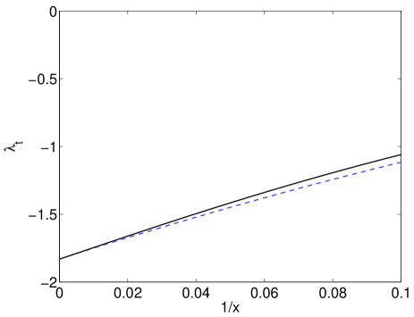
Figure 3: Two-particle translational self-diffusion virial coefficient $\lambda_{t}(x)$. Our precise results for porous particles (solid line) are well-approximated by the annulus model (dashed line).

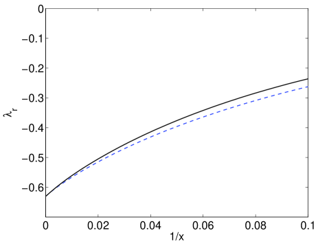
Figure 4: Two-particle rotational self-diffusion virial coefficient $\lambda_{r}(x)$. Our precise results for porous particles (solid line) are well-approximated by the annulus model (dashed line).

IV Annulus model

In the annulus model FelderhofCichocki , a particle suspended in a viscous fluid is characterized by two radii, $a_{<}$ and $a_{>}$. Its hydrodynamic interactions are governed by the smaller radius $a_{<}$. In addition, there exist also direct pair interactions. Two particles cannot come too close to each other, with the no-overlap radius equal to $a_{>}$. For such a model, the first-order virial expansion of transport coefficients has been performed with respect to the volume fraction $\phi_{>}=(4\pi/3)na_{>}^{3}$. The corresponding first-order virial coefficients $\lambda^{A}=\lambda^{A}_{t},\lambda_{K}^{A},\lambda^{A}_{r}$ have been evaluated as functions of $\epsilon$, where

$$\epsilon = \dfrac{a_{>}-a_{<}}{a_{<}}.$$ (31)

The method used to determine $\lambda^{A}$ is described in Appendix B. The calculated values are listed in Table 2.

Table 2: First-order virial coefficients $\lambda^{A}_{t}$, $\lambda_{K}^{A}$ and $\lambda^{A}_{r}$ for the short-time translational self-diffusion, sedimentation and rotational self-diffusion, respectively, for a suspension of the annulus particles.

$\epsilon$	$\lambda^{A}_{t}$	$\lambda_{K}^{A}$	$\lambda^{A}_{r}$
0.00	-1.8315	-6.5464	-0.63055
0.01	-1.7523	-6.4601	-0.56666
0.02	-1.6793	-6.3769	-0.51671
0.03	-1.6109	-6.2962	-0.47417
0.04	-1.5466	-6.2179	-0.43699
0.05	-1.4860	-6.1419	-0.40402
0.06	-1.4286	-6.0680	-0.37451
0.07	-1.3743	-5.9962	-0.34791
0.08	-1.3228	-5.9263	-0.32381
0.09	-1.2739	-5.8582	-0.30189
0.10	-1.2274	-5.7918	-0.28187
0.11	-1.1832	-5.7272	-0.26354
0.13	-1.1008	-5.6027	-0.23122
0.18	-0.9253	-5.3166	-0.16974
0.24	-0.7595	-5.0135	-0.12034
0.31	-0.6111	-4.7051	-0.08296
0.45	-0.4093	-4.1986	-0.04242
0.66	-0.2401	-3.6278	-0.01775

Now we are going to compare the first-order virial coefficients, calculated in the previous section for porous particles, with the corresponding results, obtained in this section for the annulus model, called also the hydrodynamic radius model (HRM). A similar comparison has been done in Ref. ACENW-visco-JCP:10 for the effective viscosity. The key concept in this procedure is the hydrodynamic radius of a porous particle. For the translational diffusion (self-diffusion and sedimentation), the hydrodynamic radius $a_{\text{eff}}^{t}$ is obtained from the single-particle translational diffusion coefficient, with the use of the relation,

$$D_{0}^{t} = \dfrac{k_{B}T}{6\pi\eta_{0}a_{\text{eff}}^{t}}.$$ (32)

The dependence of $a_{\text{eff}}^{t}$ on the porosity parameter $x$ follows from Eqs. (7) and (9), which determine the translational diffusion coefficient of a single porous particle Brinkman:47d ; DebyeBueche:48 ; RFJ:78 , and Eq. (LABEL:A1), which specifies the scattering coefficient $A_{10}$. Explicitly,

$${a_{\text{eff}}^{t}}(x) = a\,\dfrac{2x^{2}(x-\tanh(x))}{2x^{3}+3(x-\tanh(x))}.$$ (33)

For the rotational self-diffusion, the hydrodynamic radius $a_{\text{eff}}^{r}$ is obtained from the rotational diffusion coefficient of a single porous particle FelderhofDeutch:75 ; RFJ:78 , with the use of the relation,

$$D_{0}^{r} = \dfrac{k_{B}T}{8\pi\eta_{0}(a_{\text{eff}}^{r})^{3}}.$$ (34)

The dependence of $a_{\text{eff}}^{r}$ on the porosity parameter $x$ follows from Eqs. (26) and (28), with the scattering coefficient $A_{11}$ given by Eq. (39). As the result,

$${a_{\text{eff}}^{r}}(x) = a\,\left[1+\dfrac{3}{x^{2}}-\dfrac{3\coth(x)}{x}\right]^{1/3}.$$ (35)

For large $x$,

$${a_{\text{eff}}^{r}}(x) = {a_{\text{eff}}^{t}}(x)+{\cal O}\left(1/x^{2}\right).$$ (36)

A porous particle of radius $a$ and the porosity parameter $x$ is modeled as an annulus particle, see Fig. 5, by matching its geometrical radius $a$ to the annulus no-overlap radius $a_{>}=a$. The smaller annulus radius $a_{<}=a_{\text{eff}}$ is determined by the effective hydrodynamic radius $a_{\text{eff}}$, given in Eqs. (33)-(35).

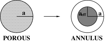
Figure 5: The annulus (or hydrodynamic radius) model of a porous particle.

In this way, the annulus parameter $\epsilon$, defined in Eq. (31), becomes the following function of $x$,

$$\epsilon(x) = \dfrac{a-a_{\text{eff}}(x)}{a_{\text{eff}}(x)},$$ (37)

with $a_{\text{eff}}(x)$ determined by Eqs. (33) and (35).

In Figs. 2-4, the annulus coefficients $\lambda^{A}(\epsilon)$, with $\epsilon(x)$ specified by Eq. (37) (dashed lines) are compared to the porous-particle virial coefficients $\lambda(x)$ (solid lines). For the sedimentation coefficient, the annulus model is accurate, with a half-percent relative accuracy already at $x=20$ and a reasonable 3% precision at $x=5$. For the translational self-diffusion, the annulus model is less accurate, but still it gives only a 2% error for $x=20$, and a 5% error for $x=10$, and a 7% error for $x=5$. The least accurate is the annulus prediction for the rotational self-diffusion, with a 5% error for $x=20$ and a 11% error for $x=10$. Summarizing, the annulus model (HRM) approximates well the first virial coefficients of porous particles suspensions, in the range of intermediate and small particle permeability (i.e. for moderate and large values of $x$).

V Conclusions

In this paper, the short-time diffusion properties of dilute suspensions of uniformly porous spherical particles have been investigated. The first-order virial coefficients $\lambda$ of the diffusion and sedimentation coefficients have been evaluated as functions of permeability. Values of $\lambda$ are well-approximated by the annulus (hydrodynamic radius) model, if the parameter $x$ is sufficiently large, i.e. the permeability is sufficiently low. Systematically, the annulus approximation slightly underestimates the virial coefficients of porous particles suspensions. For rotational diffusion, a reasonable 5% accuracy of this model is reached at $x\gtrsim 20$. For translational diffusion (collective and self), the comparable or even better 3-5% precision is obtained already for $x\gtrsim 10$. For the sedimentation coefficient, the accuracy is even higher (a 3% precision already at $x=5$), owing to much larger absolute values of $\lambda_{K}=8+\lambda_{C}$.

The annulus model is expected to work well also at larger volume fractions, if the porosity parameter $x$ is sufficiently large. The accuracy of this approximation at larger volume fractions will be investigated in a separate publication. Moreover, the annulus model is also useful to estimate diffusion and shear viscosity coefficients of suspensions made of particles characterized by a different internal structure, such as the core-shell. This problem will be the subject of a future study.

Appendix A Scattering coefficients

The scattering coefficients for a uniformly permeable sphere with $x=\kappa a$, where $a$ is the sphere radius and $1/\kappa$ is the hydrodynamic penetration depth, have the form RFJ:78 ,

$$A_{l0} = \frac{(2l\!+\!1)g_{l}(x)}{2g_{l-2}(x)}\left[1+\frac{l(2l\!-\!1)(2l\!+\!1)g_{l}(x)}{(l\!+\!1)x^{2}g_{l-2}(x)}\right]^{-1}\!a^{2l-1},$$

$$A_{l1} = \frac{g_{l+1}(x)}{g_{l-1}(x)}a^{2l+1},$$ (39)

$$A_{l2} = \left[\frac{2l\!+\!3}{2l\!-\!1}+\frac{2(2l\!+\!1)(2l\!+\!3)}{(l\!+\!1)x^{2}}\right]a^{2}A_{l0}-\frac{2l\!+\!3}{2l\!-\!1}a^{2l+1},$$

$$B_{l2} = \left[1+\frac{2(2l-1)(2l\!+\!1)}{(l+1)x^{2}}\right]a^{2}A_{l2}-a^{2l+3},$$ (41)

where $l=1,2,...$ and $g_{l}(x)=\sqrt{\pi/2x}I_{l+1/2}(x)$ is the modified spherical Bessel function of the first kind.

Appendix B The annulus (hydrodynamic radius) model

For a suspension of particles described by the annulus (hydrodynamic radius) model, the virial coefficients $\lambda^{A}$ are functions of the model parameter $\epsilon$, defined by Eq. (31) and listed in Table 2. In this Appendix, we explain how these values have been evaluated.

The first-order virial expansion of $D_{t}/D_{0}^{t}$, $D_{C}/D_{0}^{t}$, $K$ and $D_{r}/D_{0}^{r}$, can be performed with the use of $\phi_{<}=(4\pi/3)na_{<}^{3}$, or $\phi_{>}$ defined by the analogical expression,

$$1+\lambda^{A}(\epsilon)\phi_{>}+{\cal O}\left(\phi_{>}^{2}\right) = 1+\bar{\lambda}^{A}(\epsilon)\phi_{<}+{\cal O}\left(\phi_{<}^{2}\right).\hskip 25.6073pt$$ (42)

Therefore,

$$\lambda^{A}(\epsilon) = \dfrac{\bar{\lambda}^{A}(\epsilon)}{(1+\epsilon)^{3}}.$$ (43)

To evaluate $\bar{\lambda}^{A}(\epsilon)$, we now introduce the dimensionless interparticle distance as $R=r/2a_{<}$, and we replace the pair distribution function from Eq. (12) by the following expression,

$$g_{0}(R) = \left\{\begin{array}[]{ll}0&\mbox{ for }\;R\leq 1+\epsilon,\\ 1&\mbox{ for }\;R>1+\epsilon.\end{array}\right.,$$ (46)

which corresponds to the no-overlap condition at a larger radius $a_{>}$. Then, we apply the Eqs. (14), (18) and (29), taken in the non-permeable hard-sphere limit, $x=\infty$. We obtain the following expressions,

$$\bar{\lambda}^{A}_{t}(\epsilon)\!\! = \!\!8\int_{1+\epsilon}^{+\infty}J_{t}(R)R^{2}dR$$ (47)

$$= \lambda_{t}^{\text{hs}}-8\int_{1}^{1+\epsilon}J_{t}(R)R^{2}dR,$$

$$\bar{\lambda}^{A}_{K}(\epsilon)\!\! = \!\!\frac{2}{5a_{<}^{3}}A_{12}^{\text{hs}}-\frac{4}{a_{<}}A_{10}^{\text{hs}}(1+\epsilon)^{2}$$ (48)

$$+ 8\int_{1+\epsilon}^{+\infty}J_{K}(R)R^{2}dR$$

$$= \lambda_{K}^{\text{hs}}-8\int_{1}^{1+\epsilon}\bar{J}_{K}(R)R^{2}dR,$$

$$\bar{\lambda}^{A}_{r}(\epsilon)\!\! = \!\!8\int_{1+\epsilon}^{+\infty}J_{r}(R)R^{2}dR$$ (49)

$$= \lambda_{r}^{\text{hs}}-8\int_{1}^{1+\epsilon}J_{r}(R)R^{2}dR,$$

where

$$\bar{J}_{K}(R)=\frac{1}{\mu_{0}^{t}}\mbox{Tr}\left[\bm{\mu}_{11}^{tt(2)}(\mathbf{R})+\bm{\mu}_{12}^{tt(2)}(\mathbf{R})\right].$$ (50)

In this Appendix, all the mobility coefficients, the associated functions $J$, and the superscript ${}^{\text{hs}}$, refer to the hard spheres with the stick boundary conditions.

The above formulas have been applied to compute the functions ${\lambda}^{A}_{t}(\epsilon)$, ${\lambda}^{A}_{K}(\epsilon)$ and ${\lambda}^{A}_{r}(\epsilon)$, listed in Table 2. The functions $\bar{\lambda}^{A}_{t}(\epsilon)$, $\bar{\lambda}^{A}_{K}(\epsilon)$ and $\bar{\lambda}^{A}_{r}(\epsilon)$ have been also evaluated and listed in Ref. Cichocki:2010 , where they have been applied to model diffusion and rheology of particles with a hard solid core and a thin porous shell.

References

- (1) B. Cichocki, M.L. Ekiel-Jeżewska and E. Wajnryb, “Lubrication corrections for three-particle contribution to short-time self-diffusion coefficients in colloidal dispersions.” J. Chem. Phys. 111, 3265 (1999).
- (2) B. Cichocki, M.L. Ekiel-Jeżewska, P. Szymczak and E. Wajnryb, “Three-particle contribution to sedimentation and collective diffusion in hard-sphere suspensions”. J. Chem. Phys. 117, 1231 (2002).
- (3) B. Cichocki, M.L. Ekiel-Jeżewska and E. Wajnryb, “Three-particle contribution to effective viscosity of hard-sphere suspensions”. J. Chem. Phys. 119, 606 (2003).
- (4) A.J. Banchio and G. Nägele, “Short-time transport properties in dense suspensions: from neutral to charge-stabilized colloidal spheres”. J. Chem. Phys. 128, 104903 (2008).
- (5) C. N. Likos, S. Rosenfeldt, N. Dingenouts, M. Ballauff, P. Lindner, N. Werner, and F. Vögtle, “Gaussian effective interaction between flexible dendrimers of fourth generation: A theoretical and experimental study”. J. Chem. Phys. 117, 1869 (2002).
- (6) S. Huißmann, A. Wynveen, C.N. Likos, and R. Blaak, “The effects of pH, salt and bond stiffness on charged dendrimers”. J. Phys.: Condens. Matter 22 232101 (2010).
- (7) S. Pyett and W. Richtering, “Structures and dynamics of thermosensitive microgel suspensions studied with three-dimensional cross-correlated light scattering”. J. Chem. Phys. 122, 034709 (2005).
- (8) T. Eckert and W. Richtering, “Thermodynamic and hydrodynamic interaction in concentrated microgel suspensions: Hard or soft sphere behavior?” J. Chem. Phys. 129, 124902 (2008).
- (9) C. A. Coutinho, R. K. Harrinauth, V. K. Gupta, “Settling characteristics of composites of PNIPAM microgels and TiO2 nanoparticles”. Colloids Surf. A 318, 111 (2008).
- (10) M.H.G. Duits, P. A. Nommensen, D. van den Ende, and J. Mellema, “High frequency elastic modulus of hairy particle dispersions in relation to their microstructure”. Colloids Surf. A 183-185, 335 (2001).
- (11) G. Petekidis, J. Gapiński, P. Seymour, J. S. van Duijneveldt, D. Vlassopoulos and G. Fytas, “Dynamics of core-shell particles in concentrated suspensions”. Phys. Rev. E 69, 042401 (2004).
- (12) M. Zackrisson, A. Stradner, P. Schurtenberger and J. Bergenholtz, Langmuir 21, “Small-Angle Neutron Scattering on a Core−Shell Colloidal System: A Contrast-Variation Study”. 10835 (2005).
- (13) Z. Adamczyk, B. Jachimska, and M. Kolasińska, “Structure of colloid silica determined by viscosity measurements”. J. Colloid Interface Sci. 273, 668 (2004).
- (14) J. Masliyah, G. Neale, K. Malysa, and T. van de Ven, “Creeping Flow over a Composite Sphere: Solid Core with Porous Shell”. Chem. Eng. Science, 42, 245-253 (1987).
- (15) W. van Saarloos, “On the hydrodynamic radius of fractal aggregates”. Physica 147A, 280 (1987).
- (16) C. N. Likos, H. Löwen, M. Watzlawek, B. Abbas, O. Jucknischke, J. Allgaier, and D. Richter, “Star Polymers Viewed as Ultrasoft Colloidal Particles”. Phys. Rev. Lett. 80, 4450 (1998).
- (17) G.C. Abade, B. Cichocki, M.L. Ekiel-Jeżewska, G. Nägele and E. Wajnryb, “Short-time dynamics of permeable particles in concentrated suspensions”. J. Chem. Phys. 132, 014503 (2010).
- (18) G.C. Abade, B. Cichocki, M.L. Ekiel-Jeżewska, G. Nägele, and E. Wajnryb, “Dynamics of permeable particles in concentrated suspensions”. Phys. Rev. E 81, 020404(R) (2010).
- (19) G.C. Abade, B. Cichocki, M.L. Ekiel-Jeżewska, G. Nägele, and E. Wajnryb, “High-frequency viscosity of concentrated porous particles suspensions”. J. Chem. Phys. 133, 084906 (2010).
- (20) G.C. Abade, B. Cichocki, M.L. Ekiel-Jeżewska, G. Nägele, and E. Wajnryb, “High-frequency viscosity and generalized Stokes-Einstein relations in dense suspensions of porous particles”. J. Phys.: Condens. Matter 22, 322101 (2010).
- (21) B. Cichocki, B.U. Felderhof, K. Hinsen, E. Wajnryb, and J. Bławzdziewicz,“Friction and mobility of many spheres in Stokes flow”. J. Chem. Phys. 100, 3780 (1994).
- (22) S. Kim and S. J. Karrila. Microhydrodynamics. Principles and Selected Applications. Butterworth-Heinemann, London, 1991.
- (23) J. Happel and H. Brenner. Low Reynolds Number Hydrodynamics. Martinus Nijhoff, Dordrecht, 1986.
- (24) H.C. Brinkman, Proc. R. Dutch Acad. Sci. 50, 618, 821 (1947).
- (25) P. Debye and A.M. Bueche, “Intrinsic viscosity, diffusion, and sedimentation rate of polymers in solution.”J. Chem. Phys. 16, 573 (1948).
- (26) B. Cichocki, B. U. Felderhof and R. Schmitz, “Hydrodynamic interactions between two spherical particles.” PhysicoChemical Hydrodynamics 10, 383 (1988).
- (27) J.P. Hansen, I.R. McDonald, Theory of Simple Liquids, Academic Press, 1976.
- (28) B. Cichocki and B. U. Felderhof, “Short-time diffusion coefficients and high frequency viscosity of dilute suspensions of spherical Brownian particles.” J. Chem. Phys. 89, 1049 (1988).
- (29) G.K. Batchelor, “Sedimentation in a dilute dispersion of spheres”. J. Fluid Mech. 52, 245 (1972).
- (30) S. B. Chen and A. Cai,“Hydrodynamic interactions and mean settling velocity of porous particles in a dilute suspension”.J. Colloid Interface Sci. 217, 328 (1999).
- (31) B. Cichocki and B. U. Felderhof, “Diffusion of Brownian particles with hydrodynamic interaction and hard core repulsion.” J. Chem. Phys. 94, 556 (1991).
- (32) R. Reuland, B.U. Felderhof and R.B. Jones, “Hydrodynamic interaction of two spherically symmetric polymers”. Physica A 93, 465 (1978).
- (33) B.U. Felderhof and J.M. Deutch, “Frictional properties of dilute polymer solutions. I. Rotational friction coefficient”. J. Chem. Phys. 62, 2391 (1975).
- (34) B. Cichocki, M.L. Ekiel-Jeżewska and E. Wajnryb, “Suspensions of particles with solid core and thin permeable shell; short-time dynamics and high-frequency rheology”, to be published in Colloids Surf. A.